Progress in Drainage Pipeline Condition Assessment and Deterioration Prediction Models


Abstract
:1. Introduction
2. Drainage Pipe Condition Assessment and Deterioration Patterns
2.1. Pipeline Assessment Certification Manual (PACP)
2.2. Sewer Rehabilitation Manual (SRM)
2.3. Australian Conduit Condition Evaluation Manual (ACCEM)
2.4. Other Typical Standard
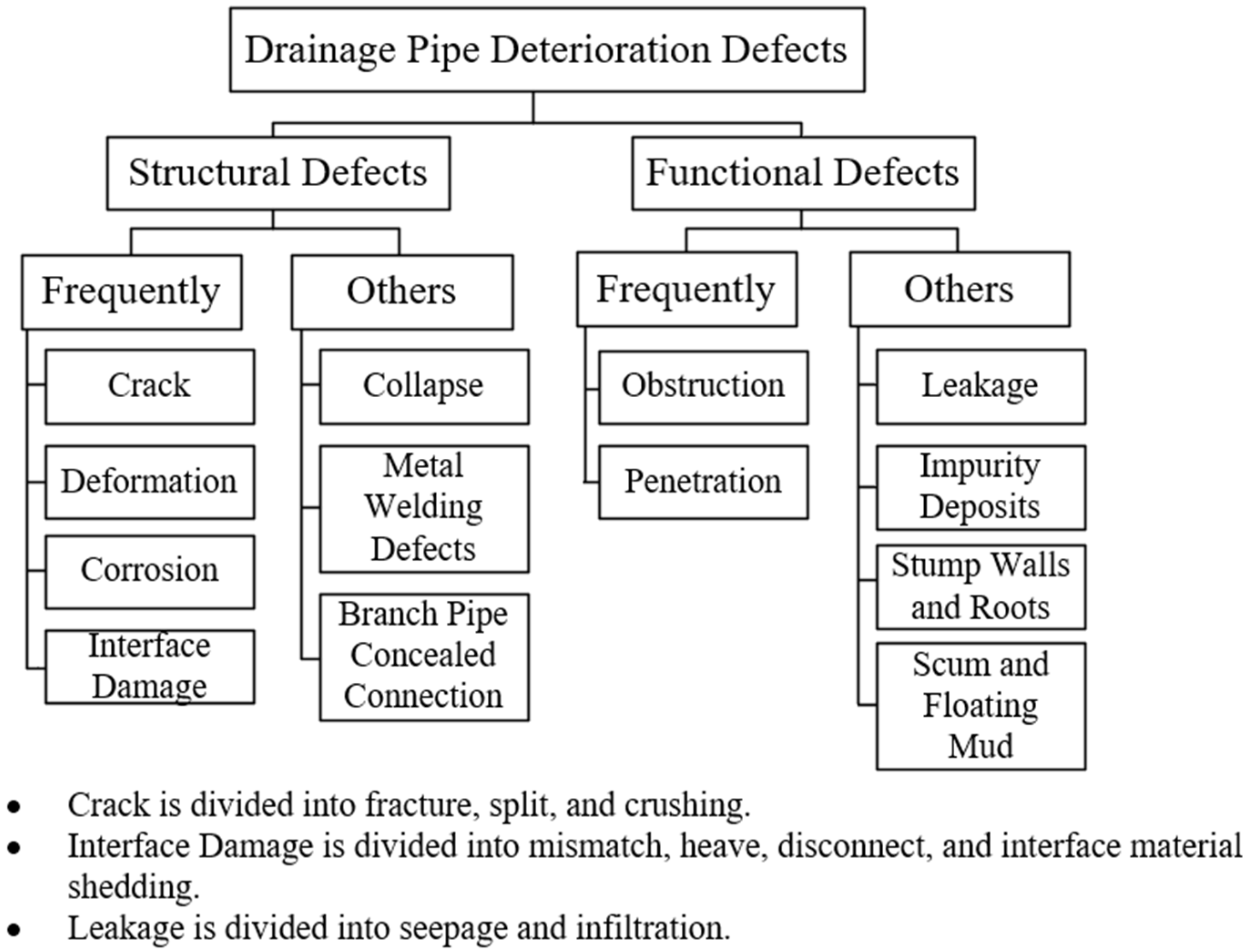
2.5. Summary and Pipeline Defects
3. Pipeline Condition Influencing Factors
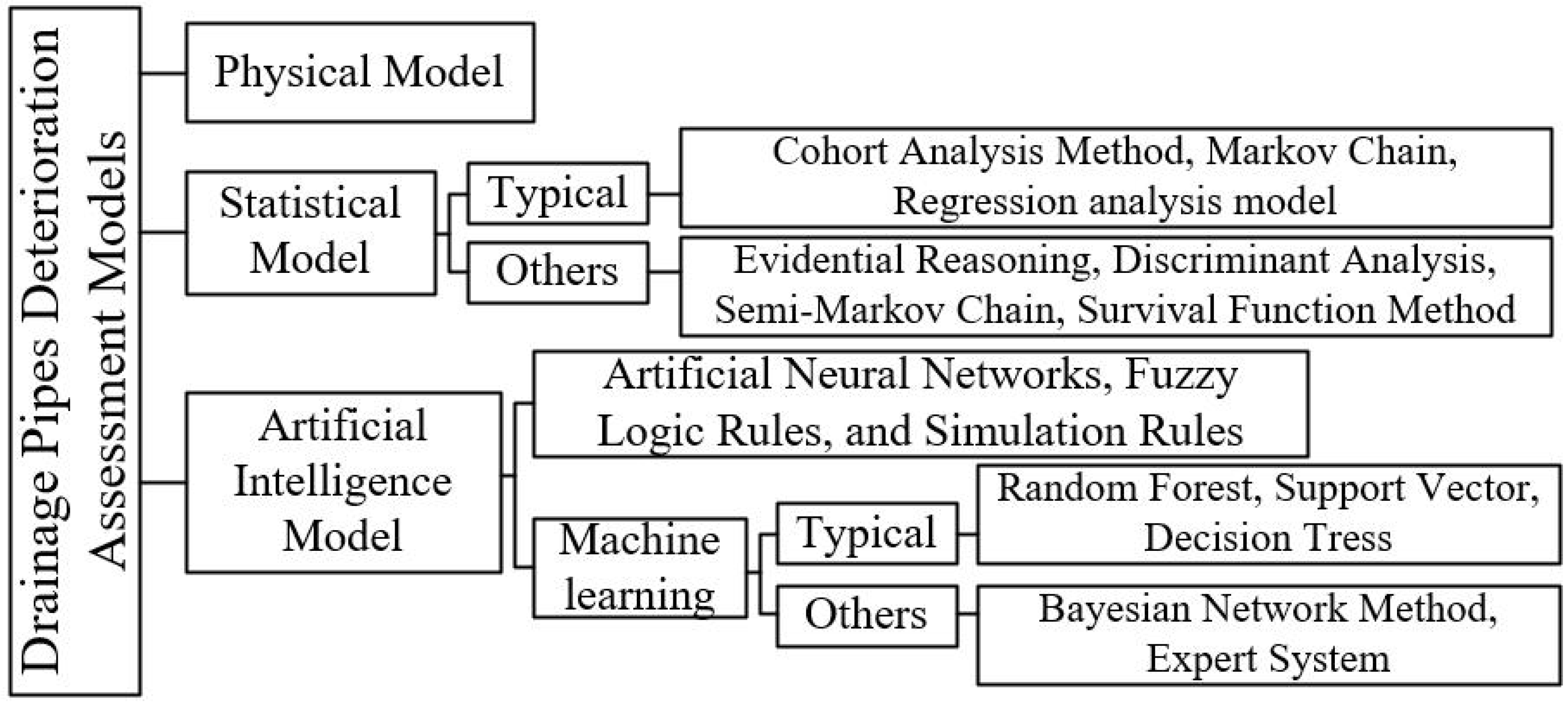
4. Drainage Pipe Condition Prediction Models
4.1. Physical Models
4.2. Statistical Models
4.2.1. Cohort Survival Models
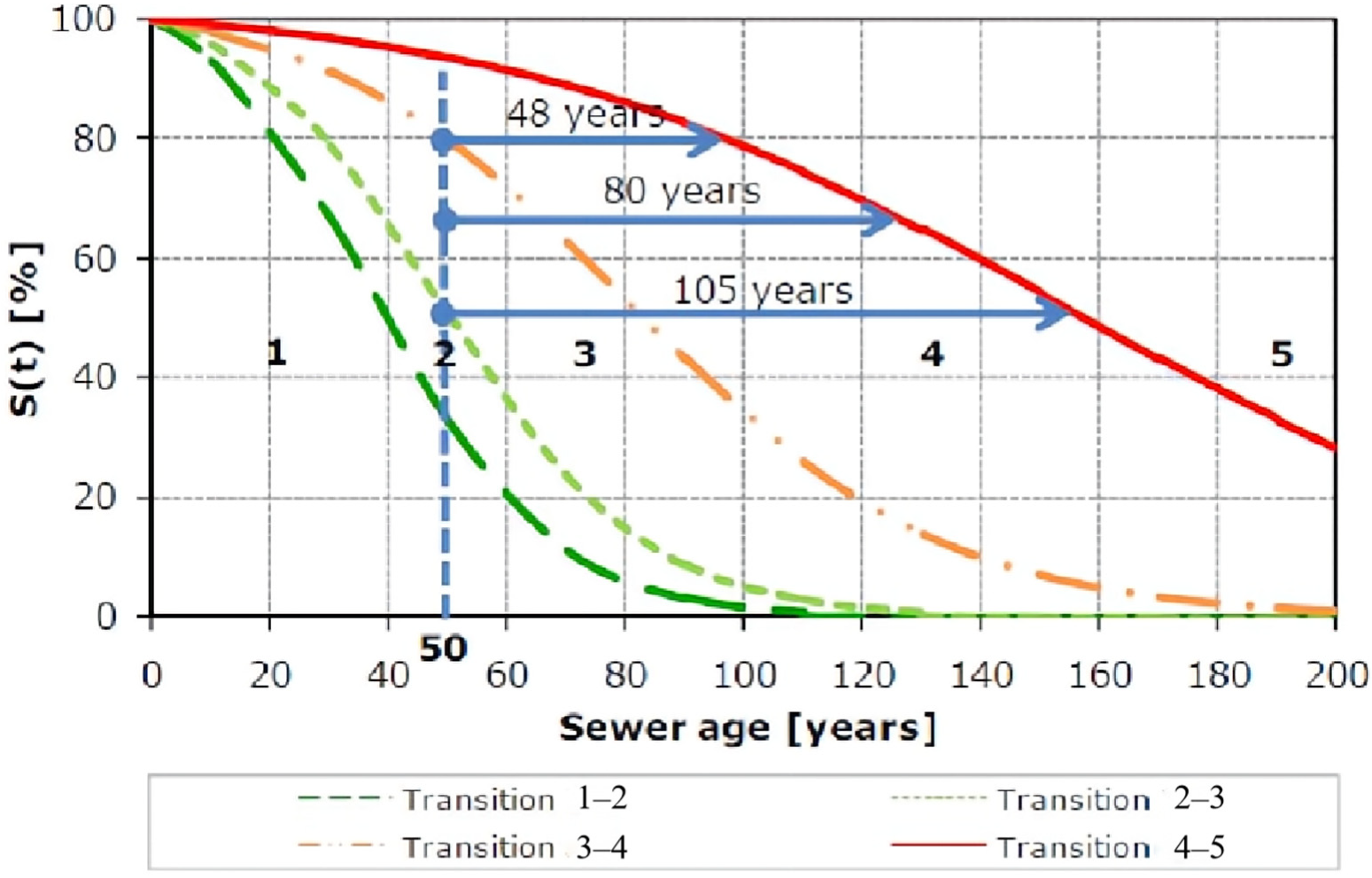
4.2.2. Markov Chains
4.2.3. Logistic Regression Models
4.2.4. Comparative Analysis of Previous Models
4.3. Artificial Intelligence (AI) Models
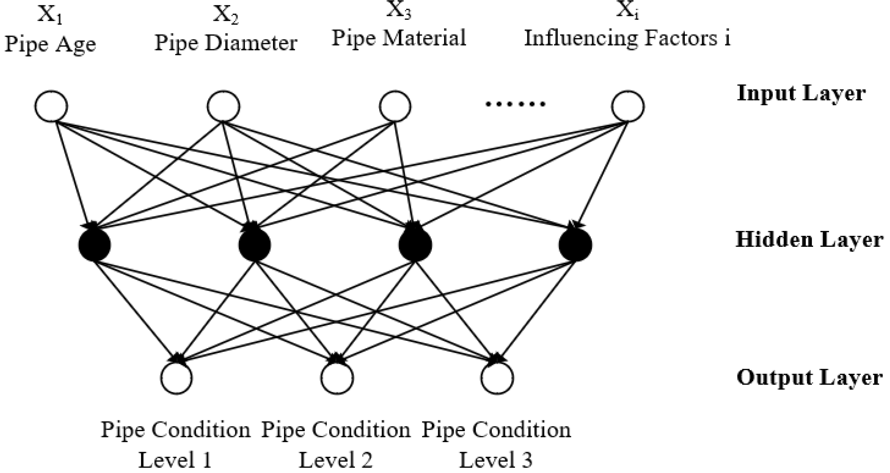
4.3.1. Artificial Neural Networks (ANNs)
- (1)
- Backpropagation neural networks
- (2)
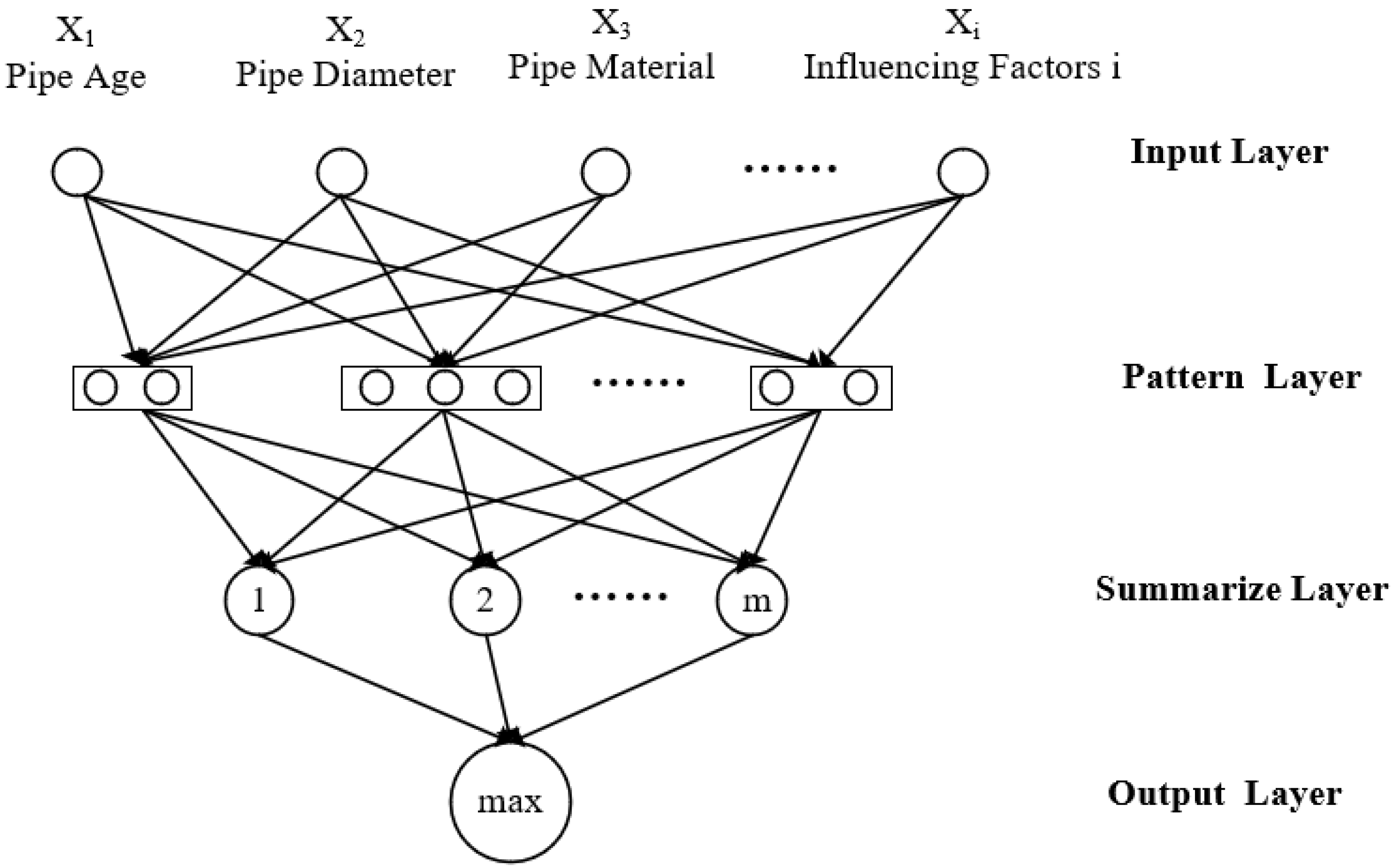
- Probabilistic neural networks
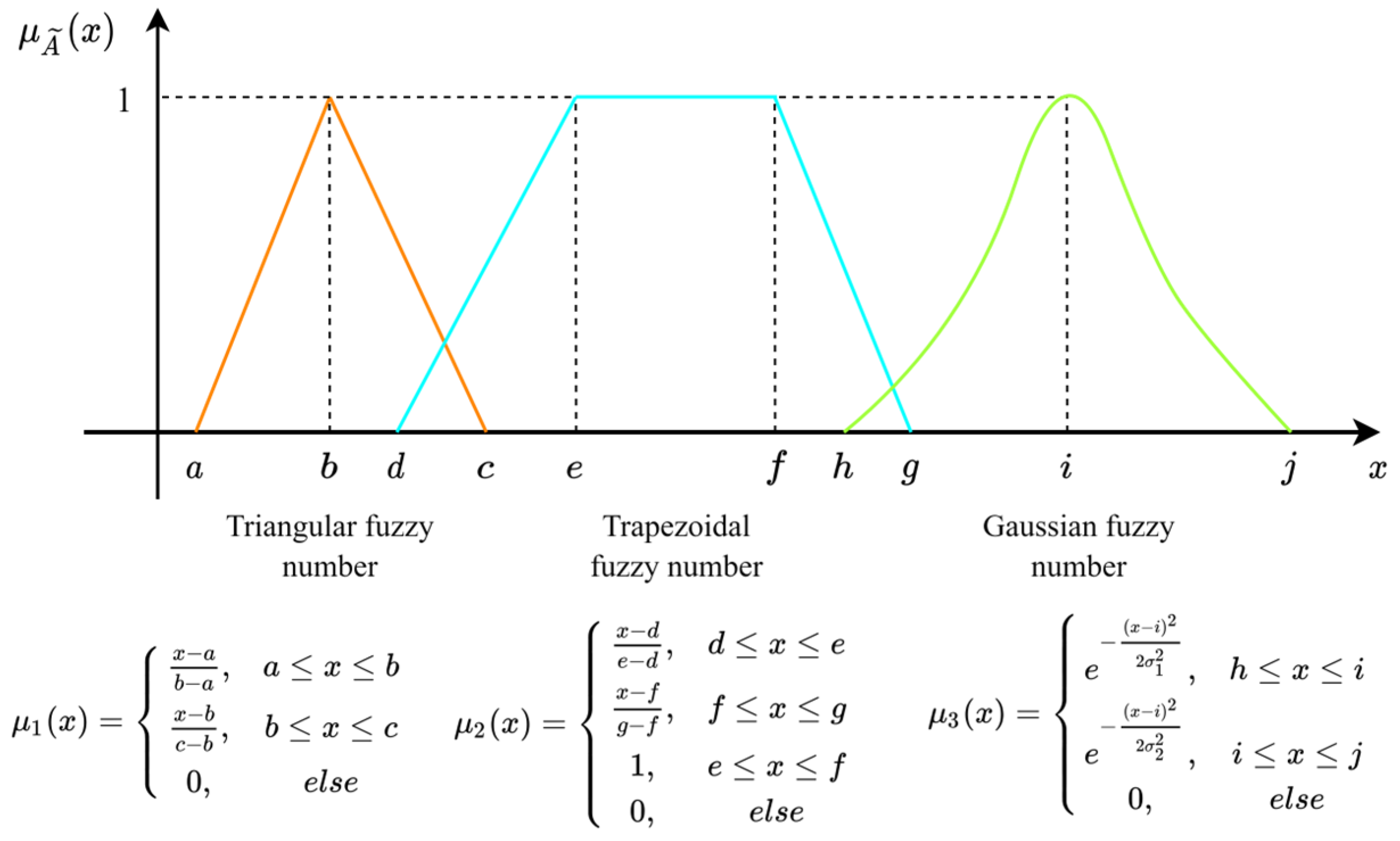
4.3.2. Fuzzy Logic Rules
4.3.3. Simulation Rules
4.3.4. Machine Learning (ML) Models
- (1)
- Random forest
- (2)
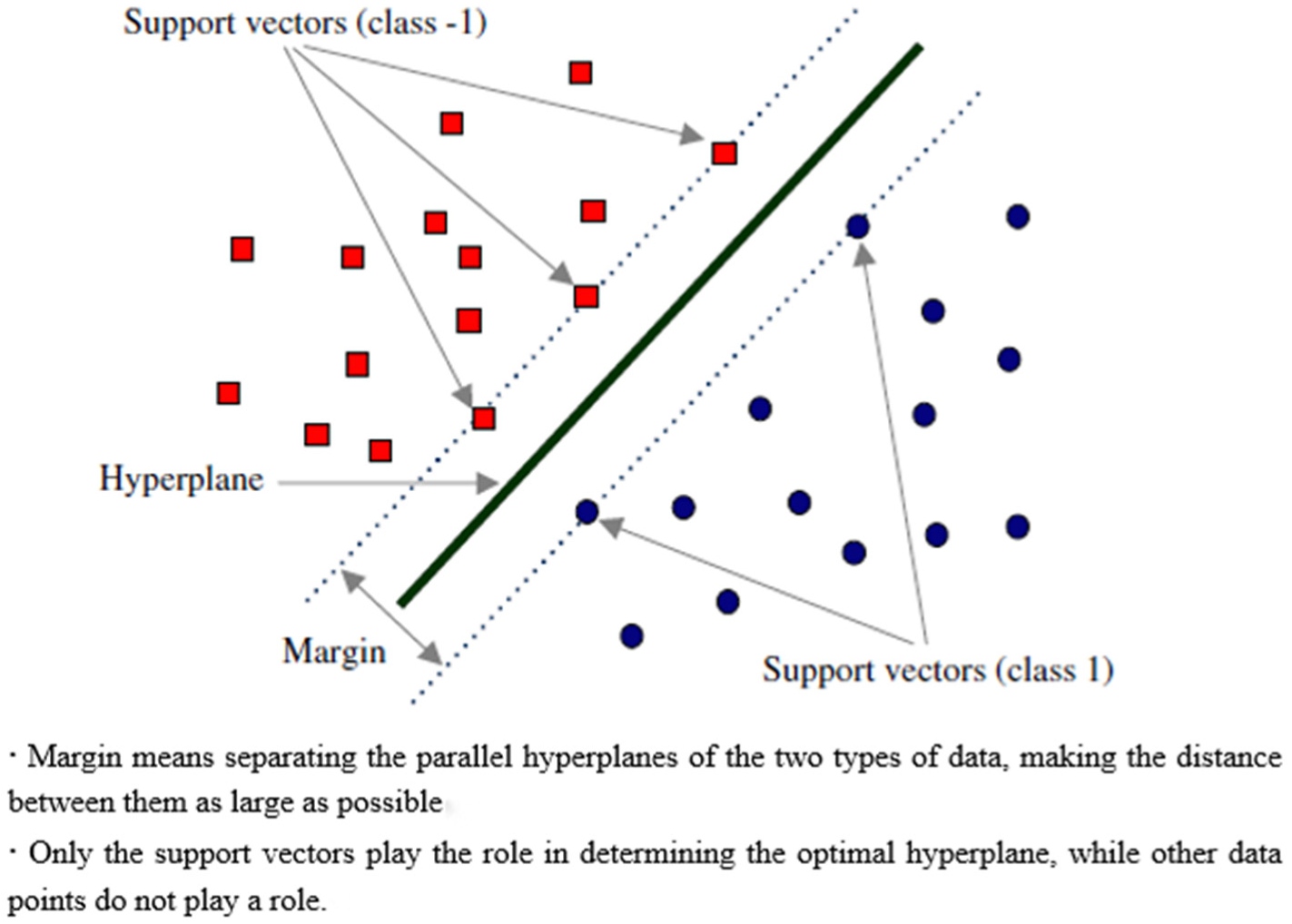
- Support vector machines (SVMs)
- (3)
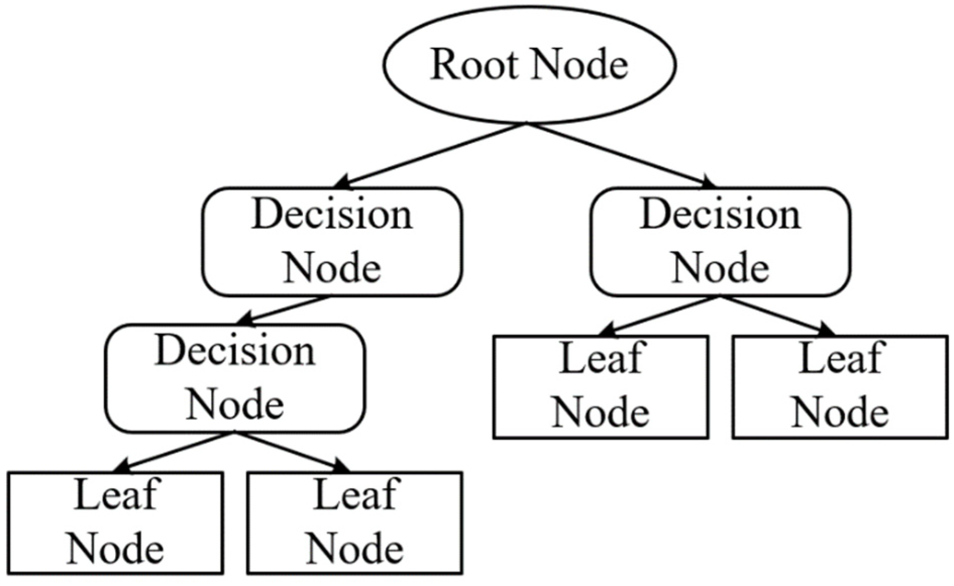
- Decision trees
5. Model Validation
5.1. Validation Methodologies
5.1.1. Goodness-of-Fit Test
5.1.2. Confusion Matrix
- True positive (TP): the model predicts the good pipe condition correctly.
- True negative (TN): the model predicts the poor pipe condition correctly.
- False positive (FP): the model predicts a poor pipe condition as a good condition.
- False negative (FN): the model predicts the active condition as a poor condition when it is not.
5.2. Validation Results in Typical Case Studies
5.2.1. Case Studies
5.2.2. Validation Result Discussion
6. Summary and Conclusions
6.1. Summary and Conclusions of Drainage Pipeline Condition Assessment
6.2. Summary and Conclusions of Deterioration Prediction Models
7. Discussion and Future Perspective
7.1. Discussion and Limitations
- The lack of investigation of the mechanism of the pipe deterioration and breakage process. The process of pipeline deterioration and breakage is very complex, and it is difficult to describe the mechanism of pipeline deterioration and breakage by employing a single discipline.
- Model building is usually limited by the availability of data. Drainage pipeline deterioration and damage prediction models often require a large amount of data to build the model, and the lack of data can lead to problems such as overfitting. A large amount of pipeline data is concentrated in the hands of pipeline operation and maintenance agencies or inspection agencies. The making available of this data would promote the in-depth study and application of the data to increase the possibility of models being used in the active operation and maintenance of pipelines.
- Existing models are difficult to widely apply. The current model is difficult to build a highly accurate and dynamically descriptive drainage pipe deterioration model because of insufficient data levels, lack of data quality, and insufficient data analysis of time span, and thus it is difficult to put into large-scale practical applications.
- Drainage pipeline health evaluation systems are difficult to unify. It is difficult to use the models and mechanisms applied in different standards and evaluation systems. Therefore, the promotion of the unification of the evaluation system in regions where pipeline health evaluation systems are relatively mature is recommended.
7.2. Future Perspective and Suggestions
- Experts from different research backgrounds should be combined to suggest interdisciplinary research on influencing factors and mechanistic models.
- The existing pipeline inspection data should be integrated, a database with regional characteristics should be established, and pipeline inspection work under different time spans should be promoted to establish a large number of databases with temporal and spatial dimensions for drainage pipe condition assessment.
- The quality of pipeline inspection data is a very important issue, and there are already researchers working on the development of an algorithm-based automatic pipeline defect detection system. The joint application of automatic pipeline defect detection and the drainage pipe deterioration prediction model is a very challenging and promising direction.
- There is an urgent need to summarize and condense manuals and standards from different countries and regions to pave the way for a cross-regional discussion of literature results.
Funding
Conflicts of Interest
References
- Grengg, C.; Mittermayr, F.; Ukrainczyk, N.; Koraimann, G.; Kienesberger, S.; Dietzel, M. Advances in concrete materials for sewer systems affected by microbial induced concrete corrosion: A review. Water Res. 2018, 134, 341–352. [Google Scholar] [CrossRef] [PubMed]
- Wang, J.; Liu, G.-H.; Wang, J.; Xu, X.; Shao, Y.; Zhang, Q.; Liu, Y.; Qi, L.; Wang, H. Current status, existent problems, and coping strategy of urban drainage pipeline network in China. Environ. Sci. Pollut. Res. 2021, 28, 43035–43049. [Google Scholar] [CrossRef] [PubMed]
- Li, Y.; Wang, W.; He, M.; Shen, T. Mechanism of Urban Black Odorous Water Based on Continuous Monitoring: A Case Study of the Erkeng Stream in Nanning. Environ. Sci. 2020, 41, 2257–2263. [Google Scholar] [CrossRef]
- Chang, H.-D.; Jin, P.-K.; Fu, B.-W.; Li, X.-B.; Jia, R.-K. Sediment Characteristics of Sewer in Different Functional Areas of Kunming. Environ. Sci. 2016, 37, 3821–3827. [Google Scholar]
- Sakai, H.; Satake, M.; Arai, Y.; Takizawa, S. Report cards for aging and maintenance assessment of water-supply infrastructure. J. Water Supply Res. Technol. 2020, 69, 355–364. [Google Scholar] [CrossRef] [Green Version]
- Huang, D.; Liu, X.; Jiang, S.; Wang, H.; Wang, J.; Zhang, Y. Current state and future perspectives of sewer networks in urban China. Front. Environ. Sci. Eng. 2018, 12, 2. [Google Scholar] [CrossRef]
- De Feo, G.; Antoniou, G.; Fardin, H.F.; El-Gohary, F.; Zheng, X.Y.; Reklaityte, I.; Butler, D.; Yannopoulos, S.; Angelakis, A. The Historical Development of Sewers Worldwide. Sustainability 2014, 6, 3936. [Google Scholar] [CrossRef] [Green Version]
- Water Research Centre. Manual of Sewer Condition Classification. Available online: https://book.douban.com/subject/12530365/ (accessed on 15 October 2022).
- Mani, M. Opportunities to Improve the UK Pipe Inspection Standard (MSCC5). VAPAR, 12 May 2022. Available online: https://www.vapar.co/opportunities-to-improve-the-uk-pipe-inspection-standard-mscc5/ (accessed on 10 September 2022).
- Tang, J.; Cao, F.; Quan, H.; Shan, Z.; Wang, J. Introduction to the status of drainage pipes in Germany. Water Wastewater Eng. 2003, 05, 4–9. [Google Scholar] [CrossRef]
- Bergue, J.-M. Réhabilitation des réseaux d’assainissement: Principaux résultats du PN RERAU. Rev. Fr. Génie Civ. 2004, 8, 51–68. [Google Scholar] [CrossRef]
- U.S. Environmental Protection Agency Office of Research and Development. Innovation and Research for Water Infrastructure for the 21st Century Research Plan. EPA/600/X-09/003, November 2009. Available online: http://www.epa.gov/nrmrl/pubs/600X09003/600X09003.pdf (accessed on 13 April 2022).
- Al-Barqawi, H.; Zayed, T. Condition Rating Model for Underground Infrastructure Sustainable Water Mains. J. Perform. Constr. Facil. 2006, 20, 126–135. [Google Scholar] [CrossRef]
- Caradot, N.; Riechel, M.; Fesneau, M.; Hernandez, N.; Torres, A.; Sonnenberg, H.; Eckert, E.; Lengemann, N.; Waschnewski, J.; Rouault, P. Practical benchmarking of statistical and machine learning models for predicting the condition of sewer pipes in Berlin, Germany. J. Hydroinform. 2018, 20, 1131–1147. [Google Scholar] [CrossRef] [Green Version]
- Laakso, T.; Kokkonen, T.; Mellin, I.; Vahala, R. Sewer Condition Prediction and Analysis of Explanatory Factors. Water 2018, 10, 1239. [Google Scholar] [CrossRef] [Green Version]
- Ana, E.; Bauwens, W.; Pessemier, M.; Thoeye, C.; Smolders, S.; Boonen, I.; De Gueldre, G. An investigation of the factors influencing sewer structural deterioration. Urban Water J. 2009, 6, 303–312. [Google Scholar] [CrossRef]
- Barton, N.A.; Farewell, T.S.; Hallett, S.H.; Acland, T.F. Improving pipe failure predictions: Factors affecting pipe failure in drinking water networks. Water Res. 2019, 164, 114926. [Google Scholar] [CrossRef] [PubMed]
- Malek Mohammadi, M.; Najafi, M.; Kermanshachi, S.; Kaushal, V.; Serajiantehrani, R. Factors Influencing the Condition of Sewer Pipes: State-of-the-Art Review. J. Pipeline Syst. Eng. Pract. 2020, 11, 03120002. [Google Scholar] [CrossRef]
- Mohammadi, M.M. Development of Condition Prediction Models for Sanitary Sewer Pipes. Ph.D. Thesis, The University of Texas at Arlington, Arlington, TX, USA, 2019. [Google Scholar]
- EPA. Condition Assessment of Underground Pipes. 2015. Available online: www.Ep.gov/nrmrl (accessed on 26 October 2021).
- Water Research Centre; Water Authorities Association. Sewerage Rehabilitation Manual; WRc Publications: Swindon, UK, 2001. [Google Scholar]
- Chughtai, F.; Zayed, T. Infrastructure Condition Prediction Models for Sustainable Sewer Pipelines. J. Perform. Constr. Facil. 2008, 22, 333–341. [Google Scholar] [CrossRef]
- Water Services Association of Australia. Conduit Inspection Reporting Code of Australia, 4th ed.; Water Services Association of Australia: Melbourne, Australia, 2020. [Google Scholar]
- Yuan, H.; Wang, X.; Yuan, J. Analysis and prevention measures of municipal drainage pipeline in south city of China. Water Wastewater Eng. 2021, 57, 112–116+122. [Google Scholar] [CrossRef]
- Anbari, M.J.; Tabesh, M.; Roozbahani, A. Risk assessment model to prioritize sewer pipes inspection in wastewater collection networks. J. Environ. Manag. 2017, 190, 91–101. [Google Scholar] [CrossRef]
- Atique, F.; Attoh-Okine, N. Using copula method for pipe data analysis. Constr. Build. Mater. 2016, 106, 140–148. [Google Scholar] [CrossRef]
- Opila, M.C. Structural Condition Scoring of Buried Sewer Pipes for Risk-Based Decision Making. Ph.D. Thesis, University of Delaware, Newark, DE, USA, 2011. [Google Scholar]
- Kley, G.; Caradot, N. D1. 2. Review of Sewer Deterioration Models; Kompetenzzentrum Wasser Berlin gGmbH: Berlin, Germany, 2013. [Google Scholar]
- Davies, J.P.; Clarke, B.A.; Whiter, J.T.; Cunningham, R.J. Factors influencing the structural deterioration and collapse of rigid sewer pipes. Urban Water 2001, 3, 73–89. [Google Scholar] [CrossRef]
- Kleiner, Y.; Rajani, B. Comprehensive review of structural deterioration of water mains: Statistical models. Urban Water 2001, 3, 131–150. [Google Scholar] [CrossRef] [Green Version]
- Kleiner, Y.; Rajani, B. Forecasting Variations and Trends in Water-Main Breaks. J. Infrastruct. Syst. 2002, 8, 122–131. [Google Scholar] [CrossRef]
- Kleiner, Y.; Rajani, B.; Wang, S. Consideration of static and dynamic effects to plan water main renewal. In Proceedings of the International Exhibition and Conference for Water Technology, Manama, Bahrain, 22–24 January 2007; pp. 1–13. [Google Scholar]
- Deterioration and Inspection of Water Distribution Systems: A Best Practice by the National Guide to Sustainable Municipal Infrastructure; Federation of Canadian Municipalities and National Research Council: Ottawa, ON, Canada, 2002; p. 34.
- Salman, B. Infrastructure management and deterioration risk assessment of wastewater collection systems. Ph.D. Thesis, University of Cincinnati, Cincinnati, OH, USA, 2010. [Google Scholar]
- Hawari, A.; Alkadour, F.; Elmasry, M.; Zayed, T. A state of the art review on condition assessment models developed for sewer pipelines. Eng. Appl. Artif. Intell. 2020, 93, 103721. [Google Scholar] [CrossRef]
- Jun, H.J.; Park, J.K.; Bae, C.H. Factors Affecting Steel Water-Transmission Pipe Failure and Pipe-Failure Mechanisms. J. Environ. Eng. 2020, 146, 04020034. [Google Scholar] [CrossRef]
- Dakers, J.L. The need for renovation or replacement of sewers. In Report of Proceedings: IPHE Training and Technical Symposium on Renovation of Sewers; University of York: York, UK, 1980. [Google Scholar]
- Khan, Z.; Zayed, T.; Moselhi, O. Structural Condition Assessment of Sewer Pipelines. J. Perform. Constr. Facil. 2010, 24, 170–179. [Google Scholar] [CrossRef]
- Ariaratnam, S.T.; El-Assaly, A.; Yang, Y. Assessment of Infrastructure Inspection Needs Using Logistic Models. J. Infrastruct. Syst. 2001, 7, 160–165. [Google Scholar] [CrossRef]
- Tran, D.H.; Perera, B.J.C.; Ng, A. Comparison of Structural Deterioration Models for Stormwater Drainage Pipes. Comput. Civ. Infrastruct. Eng. 2009, 24, 145–156. [Google Scholar] [CrossRef]
- Hu, Y.; Hubble, D.W. Factors contributing to the failure of asbestos cement water mains. Can. J. Civ. Eng. 2007, 34, 608–621. [Google Scholar] [CrossRef]
- Lubini, A.T.; Fuamba, M. Modeling of the deterioration timeline of sewer systems. Can. J. Civ. Eng. 2011, 38, 1381–1390. [Google Scholar] [CrossRef]
- Hawari, A.; Alkadour, F.; Elmasry, M.; Zayed, T. Simulation-Based Condition Assessment Model for Sewer Pipelines. J. Perform. Constr. Facil. 2017, 31, 04016066. [Google Scholar] [CrossRef]
- Ayoub, G.; Azar, N.; El Fadel, M.; Hamad, B. Assessment of hydrogen sulphide corrosion of cementitious sewer pipes: A case study. Urban Water J. 2004, 1, 39–53. [Google Scholar] [CrossRef]
- Jeong, H.S.; Baik, H.-S.; Abraham, D.M. An Ordered Probit Model Approach for Developing Markov Chain Based Deterioration Model for Wastewater Infrastructure Systems. In Pipelines 2005: Optimizing Pipe-line Design, Operations, and Maintenance in Today’s Economy; ASCE Library: Reston, VA, USA, 2005; pp. 649–661. [Google Scholar] [CrossRef]
- Tran, D.H.; Ng, A.W.M.; Perera, B.J.C.; Burn, S.; Davis, P. Application of probabilistic neural networks in modelling structural deterioration of stormwater pipes. Urban Water J. 2006, 3, 175–184. [Google Scholar] [CrossRef] [Green Version]
- O’reilly, M.P.; Rosbrook, R.B.; Cox, G.C.; McCloskey, A. Analysis of Defects in 180 km of Pipe Sewers in Southern Water Authority—TRRL Res. Rep., Art. no. RR 172. 1989. Available online: https://trid.trb.org/view/307352 (accessed on 25 April 2022).
- Harvey, R.R.; McBean, E.A. Comparing the utility of decision trees and support vector machines when planning inspections of linear sewer infrastructure. J. Hydroinform. 2014, 16, 1265–1279. [Google Scholar] [CrossRef] [Green Version]
- The History of the Newark Sewer System. Available online: https://www.oldnewark.com/histories/sewersystem.php (accessed on 22 May 2022).
- Jesson, D.; Farrow, J.; Mulheron, M.; Nensi, T.; Smith, P. Achieving Zero Leakage by 2050: Basic Mechanisms of Bursts and Leakage; University of Surrey: Guildford, UK, 2017. [Google Scholar]
- Arsénio, A.M.; Pieterse, I.; Vreeburg, J.; De Bont, R.; Rietveld, L. Failure mechanisms and condition assessment of PVC push-fit joints in drinking water networks. J. Water Supply Res. Technol.-AQUA 2013, 62, 78–85. [Google Scholar] [CrossRef]
- Bruaset, S.; Sægrov, S. An Analysis of the Potential Impact of Climate Change on the Structural Reliability of Drinking Water Pipes in Cold Climate Regions. Water 2018, 10, 411. [Google Scholar] [CrossRef] [Green Version]
- Hou, B.; Xiao, H.; Wu, S. Failure prediction model of water distribution pipelines considering weather factors. J. Harbin Inst. Technol. 2022, 54, 8–16. [Google Scholar]
- Mordak, J.; Wheeler, J. Deterioration of Asbestos Cement Water Mains: Final Report to the Department of the Environment; WRc Engineering: Swindon, UK, 1988. [Google Scholar]
- Farewell, T.S.; Hallett, S.H.; Hannam, J.A.; Jones, R.J. Soil Impacts on National Infrastructure in the United Kingdom; Cranfield University: Cranfield, UK, 2012. [Google Scholar]
- Wirahadikusumah, R.; Abraham, D.; Iseley, T. Challenging Issues in Modeling Deterioration of Combined Sewers. J. Infrastruct. Syst. 2001, 7, 77–84. [Google Scholar] [CrossRef]
- Yahaya, N.Y.N.; Lim, K.L.K.; Noor, N.N.N.; Othman, S.O.S.; Abdullah, A.A.A. Effects of clay and moisture content on soil-corrosion dynamic. Malays. J. Civ. Eng. 2011, 23, 24–32. [Google Scholar]
- Pritchard, O.G.; Hallett, S.H.; Farewell, T.S. Soil impacts on UK infrastructure: Current and future climate. Proc. Inst. Civ. Eng.—Eng. Sustain. 2014, 167, 170–184. [Google Scholar] [CrossRef]
- Gao, Y. Systematic Review for Water Network Failure Models and Cases. Master’s Thesis, University of Arkansas, Fayetteville, AR, USA, 2017; p. 64. [Google Scholar]
- Mohammadi, M.M.; Najafi, M.; Tabesh, A.; Riley, J.; Gruber, J. Condition Prediction of Sanitary Sewer Pipes. In Pipelines 2019: Condition Assessment, Construction, and Rehabilitation; American Society of Civil Engineers: Reston, VA, USA, 2019; pp. 117–126. [Google Scholar] [CrossRef]
- Salman, B.; Salem, O. Modeling Failure of Wastewater Collection Lines Using Various Section-Level Regression Models. J. Infrastruct. Syst. 2012, 18, 146–154. [Google Scholar] [CrossRef]
- Hahn, M.A.; Palmer, R.N.; Merrill, M.S.; Lukas, A.B. Expert System for Prioritizing the Inspection of Sewers: Knowledge Base Formulation and Evaluation. J. Water Resour. Plan. Manag. 2002, 128, 121–129. [Google Scholar] [CrossRef] [Green Version]
- Clark, R.M.; Stafford, C.L.; Goodrich, J.A. Water Distribution Systems: A Spatial and Cost Evaluation. J. Water Resour. Plan. Manag. Div. 1982, 108, 243–256. [Google Scholar] [CrossRef]
- Goulter, I.C.; Kazemi, A. Spatial and temporal groupings of water main pipe breakage in Winnipeg. Can. J. Civ. Eng. 1988, 15, 91–97. [Google Scholar] [CrossRef]
- Najafi, M. Pipeline Infrastructure Renewal and Asset Management; McGraw-Hill Education: New York, NY, USA, 2016. [Google Scholar]
- Rezaei, H.; Ryan, B.; Stoianov, I. Pipe Failure Analysis and Impact of Dynamic Hydraulic Conditions in Water Supply Networks. Procedia Eng. 2015, 119, 253–262. [Google Scholar] [CrossRef] [Green Version]
- Martinezcodina, A.; Castillo, M.; González-Zeas, D.; Garrote, L. Pressure as a predictor of occurrence of pipe breaks in water distribution networks. Urban Water J. 2015, 13, 676–686. [Google Scholar] [CrossRef]
- Mohammadi, M.M.; Najafi, M.; Kaushal, V.; Serajiantehrani, R.; Salehabadi, N.; Ashoori, T. Sewer Pipes Condition Prediction Models: A State-of-the-Art Review. Infrastructures 2019, 4, 64. [Google Scholar] [CrossRef] [Green Version]
- Bao, Y.; Mays, L.W. Model for Water Distribution System Reliability. J. Hydraul. Eng. 1990, 116, 1119–1137. [Google Scholar] [CrossRef]
- Dasu, T.; Johnson, T. Exploratory Data Mining and Data Cleaning; John Wiley & Sons: Hoboken, NJ, USA, 2003. [Google Scholar]
- Yang, J. Road Crack Condition Performance Modeling Using Recurrent Markov Chains And Artificial Neural Networks. Ph.D. Thesis, University of South Florida, Tampa, FL, USA, 2004. Available online: https://digitalcommons.usf.edu/etd/1310 (accessed on 4 February 2022).
- Morcous, G.; Lounis, Z. Maintenance optimization of infrastructure networks using genetic algorithms. Autom. Constr. 2005, 14, 129–142. [Google Scholar] [CrossRef]
- Tran, H.D. Investigation of Deterioration Models for Stormwater Pipe Systems. Ph.D. Thesis, Victoria University, Melbourne, Australia, 2007. Available online: http://vuir.vu.edu.au/ (accessed on 6 February 2022).
- Ana, E.V.; Bauwens, W. Modeling the structural deterioration of urban drainage pipes: The state-of-the-art in statistical methods. Urban Water J. 2010, 7, 47–59. [Google Scholar] [CrossRef]
- Salihu, C.; Hussein, M.; Mohandes, S.R.; Zayed, T. Towards a comprehensive review of the deterioration factors and modeling for sewer pipelines: A hybrid of bibliometric, scientometric, and meta-analysis approach. J. Clean. Prod. 2022, 351, 131460. [Google Scholar] [CrossRef]
- Rajani, B.; Kleiner, Y. Comprehensive review of structural deterioration of water mains: Physically based models. Urban Water 2001, 3, 151–164. [Google Scholar] [CrossRef] [Green Version]
- König, A. CARE-S WP2 External Corrosion Model Description; SINTEF Report 66138102; SINTEF Technology and Society: Trondheim, Norway, 2005. [Google Scholar]
- Vollersten, J.; König, A. WP2 Report D6: Model Testing and Evaluation, Computer Aided Rehabilitation of Sewer Networks (Care-S); SINTEF Technology and Society: Trondheim, Norway, 2005. [Google Scholar]
- Schmidt, T. Modellierung von Kanalalterungsprozessen auf der Basis von Zustandsdaten: Modelling of sewer deterioration processes with condition data. Ph.D. Thesis, Institut für Stadtbauwesen und Straßenbau, Dresden, Germany, 2009. [Google Scholar]
- Tscheikner-Gratl, F.; Caradot, N.; Cherqui, F.; Leitão, J.P.; Ahmadi, M.; Langeveld, J.G.; Le Gat, Y.; Scholten, L.; Roghani, B.; Rodríguez, J.P.; et al. Sewer asset management—State of the art and research needs. Urban Water J. 2019, 16, 662–675. [Google Scholar] [CrossRef] [Green Version]
- Baur, R.; Zielichowski-Haber, W.; Kropp, I. Statistical analysis of inspection data for the asset manage-ment of sewer networks. In Proceedings of the 19th EJSW on Process Data and Integrated Urban Water Modeling, Lyon, France, 11–14 March 2004. [Google Scholar]
- Herz, R. Alterung und Erneuerung von Infrastrukturbeständen–ein Kohortenüberlebensmodell. Jahrb. Reg. 1994, 14, 5–29. [Google Scholar]
- Herz, R.K. Ageing processes and rehabilitation needs of drinking water distribution networks. AQUA-J. Water Supply Res. Technol. 1996, 45, 221–231. [Google Scholar]
- Horold, S. Forecasting Rehabilitation Needs: Evaluation of the AQUA WertMin Software for Service Life and Total Cost Estimation; SINTEF Technology and Society: Trondheim, Norway, 1998. [Google Scholar]
- Baik, H.-S.; Jeong, H.S.; Abraham, D.M. Estimating Transition Probabilities in Markov Chain-Based Deterioration Models for Management of Wastewater Systems. J. Water Resour. Plan. Manag. 2006, 132, 15–24. [Google Scholar] [CrossRef]
- Hörold, S.; Baur, R. Modelling sewer deterioration for selective inspection planning: Case study Dresden. In Proceedings of the 13th European junior scientist workshop, Zurich, Switzerland, 22–24 August 1999; pp. 8–12. [Google Scholar]
- Baur, R.; Herz, R. Selective inspection planning with ageing forecast for sewer types. Water Sci. Technol. 2002, 46, 389–396. [Google Scholar] [CrossRef] [PubMed]
- Ana, E.; Bauwens, W.; Pessemier, M.; Thoeye, C.; Smolders, S.; Boonen, I.; De Gueldre, G. Investigating the effects of specific sewer attributes on sewer ageing—A Belgian case study. In Proceedings of the 11th International conference on urban drainage, Edinburgh, UK, 31 August–5 September 2008. [Google Scholar]
- Laakso, T.; Kokkonen, T.; Mellin, I.; Vahala, R. Sewer Life Span Prediction: Comparison of Methods and Assessment of the Sample Impact on the Results. Water 2019, 11, 2657. [Google Scholar] [CrossRef] [Green Version]
- Tran, H.; Setunge, S.; Shi, L. Markov Chain–Based Inspection and Maintenance Model for Stormwater Pipes. J. Water Resour. Plan. Manag. 2021, 147, 04021077. [Google Scholar] [CrossRef]
- Mishalani, R.G.; Madanat, S.M. Computation of Infrastructure Transition Probabilities Using Stochastic Duration Models. J. Infrastruct. Syst. 2002, 8, 139–148. [Google Scholar] [CrossRef]
- Balekelayi, N.; Tesfamariam, S. Statistical Inference of Sewer Pipe Deterioration Using Bayesian Geoadditive Regression Model. J. Infrastruct. Syst. 2019, 25, 04019021. [Google Scholar] [CrossRef]
- Tran, H.D. Markov-Based Reliability Assessment for Hydraulic Design of Concrete Stormwater Pipes. J. Hydraul. Eng. 2016, 142, 06016005. [Google Scholar] [CrossRef]
- Hao, Y.; Ma, Y.; Jiang, J.; Xing, Z.; Ni, L.; Yang, J. An Inverse Transient Nonmetallic Pipeline Leakage Diagnosis Method Based on Markov Quantitative Judgment. Adv. Mater. Sci. Eng. 2020, 2020, 1–11. [Google Scholar] [CrossRef] [Green Version]
- Koo, D.-H.; Ariaratnam, S.T. Innovative method for assessment of underground sewer pipe condition. Autom. Constr. 2006, 15, 479–488. [Google Scholar] [CrossRef]
- Atambo, D.O.; Najafi, M.; Kaushal, V. Development and Comparison of Prediction Models for Sanitary Sewer Pipes Condition Assessment Using Multinomial Logistic Regression and Artificial Neural Network. Sustainability 2022, 14, 5549. [Google Scholar] [CrossRef]
- Kabir, G.; Balek, N.B.C.; Tesfamariam, S. Sewer Structural Condition Prediction Integrating Bayesian Model Averaging with Logistic Regression. J. Perform. Constr. Facil. 2018, 32, 04018019. [Google Scholar] [CrossRef]
- Fenner, R.A. Approaches to sewer maintenance: A review. Urban Water 2000, 2, 343–356. [Google Scholar] [CrossRef]
- Le Gat, Y. Modelling the deterioration process of drainage pipelines. Urban Water J. 2008, 5, 97–106. [Google Scholar] [CrossRef]
- Hosmer, D.W., Jr.; Lemeshow, S.; Sturdivant, R.X. Applied Logistic Regression; John Wiley & Sons: Hoboken, NJ, USA, 2013; Volume 398. [Google Scholar]
- Al-Barqawi, H.; Zayed, T. Infrastructure management: Integrated AHP/ANN model to evaluate munici-pal water mains’ performance. J. Infrastruct. Syst. 2008, 14, 305–318. [Google Scholar] [CrossRef]
- Marlow, D.; Davis, P.; Trans, D.; Beale, D.; Burn, S.; Urquhart, A. Remaining Asset Life: A State of the Art Review; Water Environment Research Foundation: Denver, CO, USA, 2009. [Google Scholar]
- Specht, D.F. Probabilistic neural networks. Neural Netw. 1990, 3, 109–118. [Google Scholar] [CrossRef]
- Ana, E. Sewer asset management. Sewer structural deterioration modelling and multicriteria decision making in sewer rehabilitation projects prioritization. Ph.D. Thesis, Vrije Universiteit Brussel, Brussels, Belgium, 2009. [Google Scholar]
- Hajmeer, M.; Basheer, I. A probabilistic neural network approach for modeling and classification of bacterial growth/no-growth data. J. Microbiol. Methods 2002, 51, 217–226. [Google Scholar] [CrossRef]
- Najafi, M.; Kulandaivel, G. Pipeline Condition Prediction Using Neural Network Models. In Pipelines 2005: Optimizing Pipeline Design, Operations, and Maintenance in Today’s Economy; ASCE Library: Reston, VA, USA, 2005; pp. 767–781. [Google Scholar] [CrossRef]
- Alsaqqar, A.S.; Khudair, B.H.; Jbbar, R.K. Rigid Trunk Sewer Deterioration Prediction Models using Multiple Discriminant and Neural Network Models in Baghdad City, Iraq. J. Eng. 2017, 23, 70–83. [Google Scholar]
- Jiang, G.; Keller, J.; Bond, P.L.; Yuan, Z. Predicting concrete corrosion of sewers using artificial neural network. Water Res. 2016, 92, 52–60. [Google Scholar] [CrossRef] [PubMed] [Green Version]
- Chang, T. Methodology and Application of Pipe Condition Assessment in Urban Water Distribution System. Master’s Thesis, Environmental Science and Engineering, Tsinghua University, Beijing, China, 2016. [Google Scholar]
- Zhou, Q.; Situ, Z.; Teng, S.; Chen, G. Intelligent Detection and Classification of Drainage Pipe Defects Based on Convolutional Neural Networks. China Water Wastewater 2021, 37, 114–118. [Google Scholar] [CrossRef]
- Zadeh, L.A. Fuzzy sets. Inf. Control 1965, 8, 338–353. [Google Scholar] [CrossRef] [Green Version]
- Ishizaka, A. Comparison of fuzzy logic, AHP, FAHP and hybrid fuzzy AHP for new supplier selection and its performance analysis. Int. J. Integr. Supply Manag. 2014, 9, 1–22. [Google Scholar] [CrossRef] [Green Version]
- Chae, M.J.; Abraham, D.M. Neuro-Fuzzy Approaches for Sanitary Sewer Pipeline Condition Assessment. J. Comput. Civ. Eng. 2001, 15, 4–14. [Google Scholar] [CrossRef]
- Kleiner, Y.; Sadiq, R.; Rajani, B. Modeling Failure Risk in Buried Pipes Using Fuzzy Markov Deterioration Process. In Pipeline Engineering and Construction: What’s on the Horizon? ASCE Library: Reston, VA, USA, 2004. [Google Scholar] [CrossRef] [Green Version]
- Li, X.; Chang, H.; Duan, C.; Zheng, Y.; Shu, S. Thermal performance analysis of a novel linear cavity receiver for parabolic trough solar collectors. Appl. Energy 2019, 237, 431–439. [Google Scholar] [CrossRef]
- De Reus, N. Assessment of Benefits and Drawbacks of Using Fuzzy Logic, Especially in Fire Control Systems; Defense Technical Information Center: Fort Belvoir, VA, USA, 1994; p. 39. [Google Scholar]
- Sagdatullin, A. Improving Automation Control Systems and Advantages of the New Fuzzy Logic Approach to Object Real-Time Process Operation. In Proceedings of the 2019 1st International Conference on Control Systems, Mathematical Modelling, Automation and Energy Efficiency (SUMMA), Lipetsk, Russia, 20–22 November 2019; pp. 256–260. [Google Scholar] [CrossRef]
- Pierreval, H. Rule-based simulation metamodels. Eur. J. Oper. Res. 1992, 61, 6–17. [Google Scholar] [CrossRef]
- Inomata, T.; Onogi, K.; Nakata, Y.; Nishimura, Y. A rule-based simulation system for discrete event systems. J. Chem. Eng. Jpn. 1988, 21, 482–489. [Google Scholar] [CrossRef]
- Ruwanpura, J.; Ariaratnam, S.T.; El-Assaly, A. Prediction models for sewer infrastructure utilizing rule-based simulation. Civ. Eng. Environ. Syst. 2004, 21, 169–185. [Google Scholar] [CrossRef]
- Bishop, C.M.; Nasrabadi, N.M. Pattern Recognition and Machine Learning; Springer: New York, NY, USA, 2006; Volume 4. [Google Scholar]
- Breiman, L. Random forests. Mach. Learn. 2001, 45, 5–32. [Google Scholar] [CrossRef] [Green Version]
- Harvey, R.R.; McBean, E.A. Predicting the structural condition of individual sanitary sewer pipes with random forests. Can. J. Civ. Eng. 2014, 41, 294–303. [Google Scholar] [CrossRef]
- Wang, X.; Chen, Z.; Zhong, X.; Lu, N. Pipeline network leakage diagnosis based on multi-source random forest fusion. J. Comput. Appl. 2018, 38, 20–23. [Google Scholar] [CrossRef]
- Li, S. Risk Assessment of Municipal Pipe Network Operation and Maintenance Based on Machine Learning. Master’s Thesis, Harbin Institute of Technology, Civil Engineering, Harbin, China, 2020. [Google Scholar] [CrossRef]
- Wang, H.; Li, J.; Yang, F. Overview of support vector machine analysis and algorithm. Appl. Res. Comput. 2014, 31, 1281–1286. [Google Scholar]
- Mashford, J.; Marlow, D.; Tran, H.; May, R. Prediction of Sewer Condition Grade Using Support Vector Machines. J. Comput. Civ. Eng. 2011, 25, 283–290. [Google Scholar] [CrossRef]
- Sousa, V.; Matos, J.P.; Matias, N. Evaluation of artificial intelligence tool performance and uncertainty for predicting sewer structural condition. Autom. Constr. 2014, 44, 84–91. [Google Scholar] [CrossRef]
- Zhou, N.; Liu, Y.; Zheng, M.; Li, H. Event-driven SVM for predicting structural condition of water supply pipelines. Water Wastewater Eng. 2021, 57, 144–149. [Google Scholar] [CrossRef]
- Chen, L.; Wang, P. Water supply pipe prediction model for first leakage time based on genetic algorithm and least squares vector machine. J. Zhejiang Univ. Technol. 2021, 49, 546–549. [Google Scholar]
- Syachrani, S.; Jeong, H.S.; Chung, C.S. Decision tree–based deterioration model for buried wastewater pipelines. J. Perform. Constr. Facil. 2013, 27, 633–645. [Google Scholar] [CrossRef]
- Chen, Q.; Qu, J.; Liu, Y.; Li, W. Rule-based Model for Aging-induced Leakage from Water Supply Pipe Network in Beijing City. China Water Wastewater 2008, 24, 52–56. [Google Scholar]
- Meydani, R.; Giertz, T.; Leander, J. Decision with Uncertain Information: An Application for Leakage Detection in Water Pipelines. J. Pipeline Syst. Eng. Pract. 2022, 13, 04022013. [Google Scholar] [CrossRef]
- Schleisinger, S.; Crosbie, R.E.; Gagné, R.E. Schlesinger Terminology for model credibility. Simulation 1979, 32, 103–104. [Google Scholar] [CrossRef]
- Maroto, A.; Riu, J.; Boqué, R.; Rius, F.X. Estimating uncertainties of analytical results using information from the validation process. Anal. Chim. Acta 1999, 391, 173–185. [Google Scholar] [CrossRef]
- Massey, F.J., Jr. The Kolmogorov-Smirnov Test for Goodness of Fit. J. Am. Stat. Assoc. 1951, 46, 68–78. [Google Scholar] [CrossRef]
- Mitchell, B. A Comparison of Chi-Square and Kolmogorov-Smirnov Tests. Area 1971, 3, 237–241. [Google Scholar]
- Anderson, T.W. Anderson-Darling Tests of Goodness-of-Fit. Int. Encycl. Stat. Sci. 2011, 1, 52–54. [Google Scholar]
- Berger, V.W.; Zhou, Y. Kolmogorov–Smirnov Test: Overview. In Wiley StatsRef: Statistics Reference Online; John Wiley & Sons, Ltd.: Hoboken, NJ, USA, 2014. [Google Scholar] [CrossRef]
- Great Learning Team. Understanding Goodness of Fit Test, Definition | What Is Goodness of Fit? Great Learning Blog: Free Resources what Matters to Shape Your Career! 28 May 2020. Available online: https://www.mygreatlearning.com/blog/understanding-goodness-of-fit-test/ (accessed on 25 December 2022).
- Frost, J. Chi-Square Goodness of Fit Test: Uses & Examples. Statistics By Jim, 6 April 2022. Available online: https://statisticsbyjim.com/hypothesis-testing/chi-square-goodness-of-fit-test/ (accessed on 25 December 2022).
- Stehman, S.V. Selecting and interpreting measures of thematic classification accuracy. Remote Sens. Environ. 1997, 62, 77–89. [Google Scholar] [CrossRef]
- Powers, D. Evaluation: From Precision, Recall and F-Factor to ROC, Informedness, Markedness & Correlation. Int. J. Mach. Learn. Technol. 2011, 2, 37–63. [Google Scholar]
- Tade, O.S. A Risk Based Approach for Proactive Asset Management of Sewer Structural Conditions in England and Wales. Ph.D. Thesis, London South Bank University, London, UK, 2018. [Google Scholar] [CrossRef]


| Manual or Standard | Country | Severity Classifications | Defect Classifications |
|---|---|---|---|
| PACP | North America | 1 to 5 (1 means the minor defects, and 5 means worse situation) | Structural defects and Operation and Maintenance defects |
| SRM | UK | 1 to 5 | Structural defects and Service defects |
| ACCEM | Australia | Used to be 1 to 3, and then revised to 1 to 5 | Structural defects and Hydraulic defects |
| CJJ181-2012 | China | 1 to 5 | Structural defects and Functional defects |
| Influencing Factors | Mechanism | |
|---|---|---|
| Physical factor | Pipe age * | The mechanism of pipe age influence can be explained by the “bathtub curve” [37]. Usually, the older the pipe is, the more likely it is to break [16,38,39]. |
| Pipe diameter * | It is generally believed that pipes with larger diameters are less prone to deterioration and breakage [29,40], and pipes with diameters less than 200 mm are more prone to breakage [41]. | |
| Pipe material * | (i) The selection of pipes has a strong historical influence [17] (ii) Concrete, PVC, and other corrosion-resistant pipes are being used more and more frequently [2], and in general, as the most widely used pipe, concrete pipes have strong corrosion resistance and a lower deterioration and breakage rate [16,42] | |
| Pipe length * | (i) The effect of pipe length on the condition of pipes is related to pipe joints and lateral structures [15,16] (ii) Longer pipes are more prone to clogging or settling [16] (iii) Bending stresses due to increased pipe length are responsible for the susceptibility of pipelines to structural breakage [15,43] | |
| Pipe slope | (i) Longer retention time of sewage in gently sloping pipes leads to the generation of large amounts of hydrogen sulfide gas in the pipes, inducing pipe breakage [16,44] (ii) Pipes with large inclined angles usually have large water flow velocities, and the water flow impacts the pipe structure, thus inducing pipe structure damage [45,46] | |
| Installation quality | There is a greater correlation between the normative standards of the pipe installation formation and the type of pipe [27,28] | |
| Pipe depth | (i) Shallow pipeline burial depth is shallow and vulnerable to ground load pressure and tree root growth [18,47] (ii) Increased burial depth of the pipeline indicates an increase in the static load overlying the pipeline while increasing the possibility of the groundwater table affecting the pipeline [38,48] | |
| Pipe shape | Typically, round pipes are more resistant to deterioration breakage than square pipes [49] | |
| Coating and lining | Coatings and linings have multiple limitations for historical reasons, and usually, coated and lined pipes are less likely to deteriorate and break down [13] | |
| Joint type | (i) The damage probability of pipe joints increases significantly with time, and after some time, the damage probability of pipe joints of some materials may even be significantly greater than that of pipe sections [50] (ii) Rigid pipe joint defects usually originate from improper installation, and the movement of the upper load is more likely to induce leakage and joint fracture in rigid joints [50] (iii) Flexible pipe joints can withstand the effects of small displacements, but improper installation or multi-directional upper load movement can lead to flexible pipe joint fracture [51] | |
| Environmental factor | Seasonality * | (i) Extreme weather and sudden climatic changes can catalyze pipe deterioration and breakage with variability in the manifestations of different pipes [17,52,53] (ii) Changes in humidity and temperature due to seasonal changes can affect the condition of the pipe, and it is generally believed that there is a significant decrease in humidity and increase in temperature in summer and autumn, leading to more vulnerable pipe breakage during this period [54,55] |
| Soil condition * | (i) Soil properties such as the type of buried soil and fracture potential of the pipeline have a great influence on the pipeline [29,56] (ii) Soil compression and consolidation drainage due to ground load movement, as well as migration loss of fine soil particles triggered by groundwater seepage, can affect the condition of the pipeline [57,58] | |
| Construction location | (i) The overlying pressure of the pipeline and the traffic pressure in the pipeline construction area jointly affect the condition of the pipeline [29,59] (ii) Construction locations with more trees or deeply buried foundations can easily trigger foreign object penetration [16,28] | |
| Groundwater level | Infiltration is likely to occur when the groundwater level is higher than the pipeline location, while the increase in pore water pressure brought about by the rising water level leads to a decrease in the effective stress of the soil, increasing the risk of breakage of the pipeline structure [29,60] | |
| Operating factor | Pipe type * | (i) Drainage pipes can be divided into sewage pipes, stormwater pipes, and rainwater pipes according to their uses, and the degree of deterioration and breakage of pipes of different use types varies greatly [29,39,61] (ii) Pipe use generally determines the quality of water in the pipe, and the quality of water affects the condition of the pipe [28,62] |
| Maintenance history * | (i) The pipeline areas where defects have occurred are prone to secondary damage, and the damage forms or triggering factors have spatial and temporal clustering with the causal mechanisms of the initial pipeline defects [63,64] (ii) Human activities during operation and maintenance can affect the pipeline condition, such as dredging before pipeline cleaning and testing [29,65] | |
| Flow rate | (i) Drainage pipes are susceptible to fatigue damage under the influence of cyclic water pressure, and the phenomenon is more obvious in pipes with defects [66] (ii) The increase in the instantaneous drainage flow rate will lead to a great impact on the pipe, and fragile parts such as pipe joints and existing pipe defects are prone to breakage as a result [67] |
| Authors | Year | Classification |
|---|---|---|
| Dasu and Johnson [70] | 2003 | Data-driven and Expert-driven models |
| Yang [71] | 2004 | Physical, Statistical, and AI models |
| Morcous and Lounis [72] | 2005 | Deterministic, Probabilistic, and Soft-Computing models |
| Tran [73] | 2007 | Model-driven and Data-driven types |
| Ana and Bauwens [74] | 2010 | Pipe group model (Consider pipe sections with similar pipeline characteristics throughout the network or in regional clusters)Pipe level model (Pipeline characteristics are used as covariates to analyze the state of a pipeline in a point area for independent analysis and evaluation of a single pipeline segment) |
| Morcous and Lounis [72], Kley and Caradot [28], Salihu et al. [75] | 2005 2013 2022 | Deterministic model Deterministic, statistical, and AI models |
| Authors | Model Name | Describe |
|---|---|---|
| König [77] | ExtCorr | Predicting external deterioration of concrete pipes by assessing soil moisture, corrosion, and cement quality |
| Vollersten and König [78] | WATS | Describe the joint mechanism of compounds in wastewater and organic transformation processes on the internal deterioration state of pipes using nonlinear differential equations |
| Model Type | Advantages | Disadvantages |
|---|---|---|
| Cohort survival model | (i) Concept is easy to understand and easy to calculate (ii) Transition curve gives a good explanation of the deterioration and damage process of the pipeline (iii) Beneficial to the cost calculation of pipeline maintenance and repair [74] | (i) The data demand is huge and usually not easy to meet [98] (ii) Pipes that have undergone deterioration and breakage are easily ignored in model calculations, resulting in large predicted pipeline life [99] |
| Markov chain | (i) The model can be greatly simplified by reducing the number of similar pipes when calibrating the transition function [28] (ii) The most likely time of pipe deterioration can be predicted, and the model is very flexible | (i) The pipeline needs to be classified and grouped, and each group of models requires sufficient data for simulation validation (ii) The conditional probability matrix is complex to build [68] |
| Logistic regression model | (i) The concept is simple and easy to understand, and the model is powerful in prediction (ii) It can analyze the degree of influence of influencing factors on the deterioration and breakage of the pipeline (iii) The model mechanism is highly explanatory and can decompose the pipeline deterioration and damage process (iv) The model can be built without the prerequisite assumptions [34,100] | (i) The data requirements are extremely high (ii) The linear nature of logistic regression is not flexible enough to identify nonlinear decision boundaries and more complex relationships [35,68] |
| Year | Authors | Describe |
|---|---|---|
| 2014 | Harvey and McBean [123] | A random forest model was developed using pipeline data from Guelph, Canada, and ROC curves were used to establish alternative cut-off points for prediction probabilities, proving that the random forest model is an “excellent” choice for predicting pipeline condition |
| 2018 | Laakso et al. [15] | A random forest model was developed with a logistic regression model, and the results showed that random forest had higher accuracy. It was also found that although deformation, root intrusion, and pipe surface defects were not significantly characterized in the set of datasets, the random forest still had higher accuracy in predicting the results of the above damage patterns |
| 2018 | Wang et al. [124] | Proposed a random forest fusion-based pipeline leakage diagnosis method, the algorithm improves the accuracy by 2.2% and 6.4% compared to the backpropagation neural network model and the D-S evidence theory model of support vector machine, respectively |
| 2020 | Li [125] | A random forest model is established based on the monitoring data of a pipeline network in a park in Suzhou, and the univariate and inter-variate analysis is used to obtain the feature importance and contribution rate, to give the decision path of the pipeline section, to improve the interpretability of the model, and to prove the superiority of the random forest algorithm |
| Year | Authors | Describe |
|---|---|---|
| 2011 | Mashford et al. [127] | A support vector machine model was established by selecting influencing factors such as pipe age, pipe diameter, road type, pipe inclination angle, pipe, soil type, etc. The accuracy of the model reached 91%, but due to the lack of sufficient data, the model still has room for improvement |
| 2014 | Harvey and Mcbean [128] | Using pipeline data from Guelph, Canada, a support vector machine model was built using selected influencing factors such as pipe age, pipe, and pipe type, with a model accuracy of 76%. |
| 2021 | Zhou et al. [129] | Combining kernel density estimation and support vector machine algorithm to construct a drainage pipe deterioration and breakage prediction model, the model accuracy reaches 91%. Applying the model to the pipeline in Yangpu District, Shanghai, it can effectively identify the pipe sections with a lower safety level |
| 2021 | Chen and Wang [130] | To solve the time-consuming problem of least squares support vector machine, an adaptive genetic algorithm is used to optimize LSSVM parameters and establish a pipeline health state prediction model with overburden depth, pipe diameter, water pressure, and road grade as inputs, and the results show that the new model takes less time to model and has better prediction capability |
| Year | Authors | Describe |
|---|---|---|
| 2008 | Chen et al. [132] | Analyze the aging and leakage data of Beijing pipelines from 1987 to 2005, apply a decision tree algorithm to develop a pipeline prediction model based on pipe age and pipe diameter, and predict the distribution of aging and leakage of pipelines in Beijing in 2008 through ArcGIS |
| 2013 | Syachrani et al. [131] | A decision tree model based on background information survey and pipe inspection data is selected for pipe age, pipe diameter, pipe length, pipe inclination, and number of trees, and the model has good performance in predicting the pipe age of drainage pipes |
| 2014 | Harvey and McBean [48] | Using pipeline data from Guelph, Canada, a decision tree and a support vector machine model were built using selected influencing factors such as pipe age, pipe, and pipe type, and the results showed that the support vector machine model was more accurate |
| 2022 | Meydani et al. [133] | A Bayesian decision model based on decision tree theory is developed to facilitate the structuring process of the initial problem in a decision process with uncertainty. Applying the model to a water distribution network architecture in Sweden, the results show that the cost of human intervention and leakage probability have a significant impact on the model performance and O&M decisions |
| Approach | Description | Application Scope | Merits |
|---|---|---|---|
| The chi-square | It evaluates whether proportions of categorical or discrete outcomes in a sample follow a population distribution with hypothesized proportions. |
|
|
| Kolmogorov-Smirnov | It assesses whether a single sample could have been sampled from a specified probability distribution |
|
|
| Anderson-Darling | It is used to compare the fit of the observed cumulative distribution function with the expected cumulative distribution function. |
|
|
| Region | Authors | Case Description | Validation Results |
|---|---|---|---|
| Australia | Tran [73] |
|
|
| USA | Salman [34] |
|
|
| UK | OS Tade [144] |
|
|
| Germany | Le Gat [99] |
|
|
| Belgium | Ana [104] |
|
|
Disclaimer/Publisher’s Note: The statements, opinions and data contained in all publications are solely those of the individual author(s) and contributor(s) and not of MDPI and/or the editor(s). MDPI and/or the editor(s) disclaim responsibility for any injury to people or property resulting from any ideas, methods, instructions or products referred to in the content. |
© 2023 by the authors. Licensee MDPI, Basel, Switzerland. This article is an open access article distributed under the terms and conditions of the Creative Commons Attribution (CC BY) license (https://creativecommons.org/licenses/by/4.0/).
Share and Cite
Zeng, X.; Wang, Z.; Wang, H.; Zhu, S.; Chen, S. Progress in Drainage Pipeline Condition Assessment and Deterioration Prediction Models. Sustainability 2023, 15, 3849. https://doi.org/10.3390/su15043849
Zeng X, Wang Z, Wang H, Zhu S, Chen S. Progress in Drainage Pipeline Condition Assessment and Deterioration Prediction Models. Sustainability. 2023; 15(4):3849. https://doi.org/10.3390/su15043849
Chicago/Turabian StyleZeng, Xuming, Zinan Wang, Hao Wang, Shengyan Zhu, and Shaofeng Chen. 2023. "Progress in Drainage Pipeline Condition Assessment and Deterioration Prediction Models" Sustainability 15, no. 4: 3849. https://doi.org/10.3390/su15043849
APA StyleZeng, X., Wang, Z., Wang, H., Zhu, S., & Chen, S. (2023). Progress in Drainage Pipeline Condition Assessment and Deterioration Prediction Models. Sustainability, 15(4), 3849. https://doi.org/10.3390/su15043849