Abstract
The reliability of a power system is considered as a critical requirement in planning and operating the system due to the increasing demand for more reliable service with a lower frequency and duration of interruption. Hence, reliability is also considered as a major challenge in the development of future power systems as they become more advanced and complex, making the accuracy of the reliability assessment dependent on several factors such as supply and load modeling. Recent studies on power systems’ reliability and stability have focused on load modeling, where loads are either assumed to be static or dynamic, by introducing significant constraints. However, the emergence of new types of loads necessitates the development of models that can incorporate them with accuracy, as this would facilitate their effective use in flow and stability simulation studies, as well as reliability analyses. In this study, dynamic loads are modeled using a feed-forward neural network where a simulation test bed is developed in MATLAB/Simulink to generate operating data used during training and validating of the neural network model. Subsequently, Electrical Transient Analyzer Program (ETAP) software is used to verify the effect of load modeling on power system reliability assessment platform. Bus 2 of Roy Billinton Test System (RBTS) is employed as a case study to investigate the sensitivity of the reliability indices, such as System Average Interruption Duration Index (SAIDI) and System Average Interruption Frequency Index (SAIFI), on the load modeling technique with mixed loads (dynamics and statics).
1. Introduction
Load modeling is a new research area in the field of power system stability and reliability. To assist in accurate power system planning and operation and yield reasonable and realistic results, simulation studies of load flow and stability must rely on accurate network models, especially with regard to the loads [1,2,3,4,5,6]. However, modern power system designs are rapidly diverging from those of traditional systems in many respects. Specifically, as new loads are being integrated into power systems, there is an urgent need to develop new techniques for load modeling. More sophisticated models would enhance our understanding of loads and provide better load representation in simulation studies. Such advancements will have a positive influence on the control, operation, and reliability of power systems. In particular, nonlinear dynamic loads, such as those of Programmable Logic Controllers (PLCs), variable-speed drives and power electronics, are becoming more common in power systems. Consequently, they increasingly contribute to the complexity of load modeling [7]. The typical approach to load modeling aimed at the evaluation of reliability indices, in which all loads are assumed to be static, should be modified. Because most loads in this technological era originate from either motors, pumps, compressors or power electronics, the use of static models to study the reliability of these systems yields highly inaccurate results [8]. The output provided by static models, although useful in allowing the designer to identify weak points and propose suitable reinforcements for a system, do not include the effects of load variations, which strongly and directly affect the system’s calculated reliability indices [9].
Many approaches to load modeling have been introduced and discussed in the pertinent literature. However, these strategies were typically aimed at testing the reliability of a power system or evaluating the costs of interruptions to customers to obtain a practical understanding of a system that will be installed or developed. Certain load modeling approaches such as time-varying or dynamic load modeling, in which the loads can randomly vary over time, provide a highly practical and accurate representation of any interrupted load in a power system [10]. These dynamic load modeling methods not only yield more accurate reliability indices than their static counterparts, but also allow the system to be designed to respond to any potential disturbances before they occur. Moreover, they permit the severity of a disturbance to be reduced when development measures cannot be applied [11].
In practice, while the data on individual loads are generally unavailable, the aggregate power transmitted through the bus can be easily measured. The resulting loads are likely a composite of static and dynamic or nonlinear loads. Consequently, various techniques have been proposed for modeling such combinations of disparate loads [12]. However, many of these techniques are based on assumed load equations, the parameters of which are estimated via curve fitting [13]. Because these methods do not accurately capture various power, voltage, and frequency phenomena, it is preferable to devise other techniques to model these loads [14,15]. Load compositions are generally characterized based on load class data, the composition of each class, and the characteristics of each load component. Loads are often grouped into residential, commercial, industrial, and sometimes agricultural loads. Industrial loads tend to be dominated by industrial motors, which are estimated to contribute 95% of all industry applications. Residential loads stem from the use of household devices and appliances and are dominated by the demand imposed by electric heating and air conditioning systems. Commercial loads are primarily associated with discharge lighting and the extensive use of space heaters and air conditioners. Finally, agricultural loads chiefly consist of irrigation loads [12].
The aforementioned load types can be further categorized based on the following considerations:
- Fast dynamics of both mechanical and electrical characteristics, e.g., induction motors
- Significant effects of under-voltage excursions, e.g., discharge lighting
- Insignificant delays and discontinuities in response to voltage faults, e.g., incandescent lighting
- Slow characteristics, e.g., electric heating
Induction motors constitute the largest percentage of the load composition at the residential, commercial, and industrial levels. They are widely used in compressors for refrigeration and air conditioning. As they require nearly uniform torque at all operational speeds, they may compromise system stability. Given that induction motors consume approximately 60–70% of the energy in typical power systems, their dynamics are typically the focus of voltage stability studies [12].
Lighting comes in various forms. However, fluorescent, mercury vapor, and sodium vapor lamps provide most industrial and street lighting and therefore constitute a significant percentage of commercial loads. They are highly susceptible to voltage variations and require at least 80% of the nominal voltage for operation. Most loads in residential areas are thermal in nature, such as loads from water heaters, ovens, and electric heating. In the industrial sector, devices such as soldering and molding machines and boilers similarly act as constant-resistance devices over short periods of time. Decreases in voltage and power do not instantaneously affect the temperature and resistance of these loads. A good example is a thermostat, which behaves like a constant power load over extended period of time [12]. Collin et al. provided an excellent summary of other load types [13]. In 1994, Bih-Yuan and colleagues applied Artificial Neural Networks (ANNs) in power system dynamic load modeling [14]. The phase voltage sequence components served as the input to the ANN, while the electric power was the output. In the ANN development, the authors used actual field data and concluded that load dynamics can be accurately identified using this method.
According to Chen and R. R. Mohler, the load modeling techniques currently employed in detecting voltage stability tend to only consider either static or quasi-static loads, thereby neglecting to account for the load dynamics [15]. To address this shortcoming, the authors adopted recurrent neural networks, as modeling the load dynamics provides a more accurate estimation relative to the outcomes of the conventional methods. When testing their approach, the authors applied the developed model on the IEEE 14 bus system. They concluded that the results obtained justify the use of the proposed neural network method that incorporates load dynamics.
Renmu and colleagues [16] developed a measurement-based composite load model comprising of a combination of a motor and static Impedance-Current-Power (ZIP) loads. All model parameters were identified from practical field measurements. The accuracy of the developed model was investigated through several case studies.
The time of day, month and season determine the load composition at a given load point at a given time. In cold regions, electric heating is in much higher demand during winter relative to summer. Likewise, in hot regions, use of air conditioning units dominates the load during the summer. Such loads are thus seasonal. Similarly, industrial and commercial loads exhibit weekly patterns. For example, some industrial processes may be preferentially conducted during evening hours and on weekends, whereas commercial loads represent larger demands corresponding to typical working hours.
Based on the aforementioned discussion, several studies modeled the static loads and the impact of load modeling on stability and reliability studies. However, as new dynamic and sophisticated load types are rapidly being introduced into the power systems, adequate and accurate models and techniques are required to address the impact of dynamic loads to better understand the system and attain more accurate reliability assessments. The contribution of this work prompted the development of a neural network-based dynamic load model and a test bed in MATLAB/Simulink to simulate the dynamic load model and to train and validate the proposed model. Subsequently, ETAP software is used to verify the effect of the proposed load model on power system reliability assessment. Bus 2 of RBTS is analyzed to investigate the sensitivity of the reliability indices, such as SAIDI and SAIFI to the proposed load modeling technique when having mixed loads (dynamics and statics).
In the following sections, a brief review of current load modeling techniques is given to identify their advantages and disadvantages. Furthermore, a simulation test bed developed in MATLAB/Simulink to produce operating data is presented, and a feed-forward neural network training method and a load model validation using the simulated data are described. Moreover, verification of the effects of various load models on the reliability of a power system is performed using the RBTS as a test bed via ETAP software. Finally, conclusions are drawn based on the results pertaining to various scenarios.
2. Standard Loads Model
Models are sets of equations that represent the relationships between the inputs and outputs of physical systems. In the context of load modeling, these equations relate the measured voltage or frequency at a load point or bus to the power consumed by the loads, both real and reactive. However, due to the high diversity and distribution of power system loads, various techniques have been devised to achieve accurate modeling [13]. Generally, load models are classified as either static or dynamic. A static load model is independent of time and relates active and reactive power values to the voltage and frequency at a particular point in time. In contrast, in dynamic modeling, the expressed relationships are immutable regardless of the point in time to which they pertain.
2.1. Static Load Models
Static loads for real and reactive power are represented by exponential or polynomial expressions. If needed, a frequency-dependent term can also be included [17]. The most common static load models are the ZIP, exponential, and frequency-independent load models. A ZIP model describes the static characteristics of a load depending on the relationship between power and voltage. The dependence of power on voltage is quadratic for a constant load, linear for a constant current, and independent for constant power. Equations (1) and (2) describe the general relationships used in this type of model [16], which correspond to a polynomial model that describes the sum of these categories.
where P0, V0, and Q0 respectively denote the nominal values of the active power, voltage, and reactive power of the system; P and Q are the load and consumed power, respectively; and a1 through a6 are the model parameters. Many static load models rely on exponential relationships, as shown below.
where np and nq are parameters that can be tuned to achieve the appropriate dependence of the load on the voltage. When np and nq are equal to 0, 1, and 2, the load model corresponds to the three respective cases of the ZIP model discussed above. In the Frequency-Dependent Load Model, as stated by Chassin et al. [9], the dependence on frequency in a static load model can be represented by multiplying Equations (1) and (2) by a frequency-dependent factor, as shown in Equation (5) below,
where f and f0 respectively denote the frequency and nominal frequency of the voltage at the bus being studied, and D is the change in the load, expressed as a percentage, divided by the percentage change in frequency. The term D(f − f0) is the frequency-sensitive load variation in the load model.
2.2. Dynamic Load Models
When static load models yield inaccurate results, dynamic load models are viable options because they allow power to be considered as a function of both voltage and time [12]. As ample literature on the types of dynamic load models exists, for brevity, it is not discussed here. Thus, only the three types of dynamic load models that pertain to the objective of this work, namely the generic non-linear dynamic model, the composite load model, and the neural network model, are described below.
Generic Nonlinear Dynamic Model: the objective of this model is the generalization of a nonlinear static model into a dynamic model. Thus, this model relies on a nonlinear dynamic differential equation that relates power and voltage shown below, which was adapted from Wong and Haque [11].
The key variables here are Pd and V. The parameters Kp and Ps are nonlinear functions of voltage that characterize the dynamic load behavior [11,14]. Under the assumption of a stepwise change in voltage from V0 to V1 over a time span t – t0, solving the differential equation results in (7).
Based on the work of Navarro (12), Wong and Haque [6] assumed an exponential recovery of the steady state as the dynamic response of the power output, and applied this generic model to many loads. A composite load model is based on representing the total load as a parallel combination of static, dynamic and induction motor loads. This model is adopted in many extant load modeling studies. Its unambiguous physical meaning makes it attractive to power engineers because the majority of power system loads are induction machines [17]. This strategy is often referred to as the “bottom-up” approach to load modeling. Although the model is complex, it yields very accurate results. The load modeling commences with models of individual components that are incorporated into load models for broader areas via an aggregation approach [18]. Equations (8) and (9) describe the procedure used to aggregate the load models at a particular bus:
where Ls, Ld, and Lm are the static, dynamic and motor loads, respectively, at a given load point. The weights of each model are represented by w1 through w3, and L denotes the composite load at the load point. Additionally, typical load curves can be generated for an area of interest by conducting surveys of the load types and classes in that area [19]. In their work, Zhang et al. [19] provided techniques for determining the load class mix from a load profile curve. Thus, the weights in (8) can be determined from the findings yielded by such a survey.
Neural networks are parallel distributed sets of connections comprising of simple processing units (neurons), which gain knowledge by learning from their environment. Neural networks are used in many applications, such as classification, regression, pattern recognition, clustering, control, and function approximation. At present, various types of neural networks are available, such as Multi-layer Feed-forward Neural Networks (MFNNs) and Radial Basis Function Neural Networks (RBFNNs). MFNNs are the most commonly used type of neural network, and they consist of an input layer, several hidden layers, and an output layer. Each layer consists of several neurons, each of which includes a summer and an activation function g. Figure 1 depicts a single neuron.
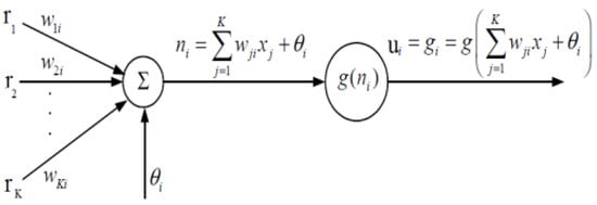
Figure 1.
Single node (neuron).
The inputs to the neuron, xj (j = 1,2,…, K), are multiplied by the weights WKi and are added to the constant bias term θi. The resulting ni is the input to the activation function g. The output of neuron i thus becomes:
By connecting several nodes in parallel and in series, an MFNN network is formed. A typical MFNN is shown in Figure 2.
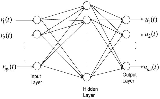
Figure 2.
Typical multi-layer feed-forward neural network (MFNN).
The neural network is trained using a back-propagation algorithm, which identifies the optimal weight biases of the neural network along the gradient decent of a cost function, given by:
where u and ur denote the actual and desired outputs, respectively. A complex non-linear relationship can be precisely modeled using a well-structured and adequately trained neural network. In this study, an MFNN was used to model a composite load.
2.3. Load Model Calibrations
Although several methods are available for calibrating load models, only the two pertinent to the present study are discussed here. When a satisfactory load model has been developed, that model must still be calibrated to yield a reasonable fit to the measured data [14]. To accomplish this, the model parameters must be adjusted. The measurement-based approach and the component-based approach are the two calibration techniques discussed in this section.
The measurement-based approach, which was adopted in this study, relies on direct measurements at the feeders and substations to uniquely determine the frequency and voltage sensitivities of the real and reactive power loads. These measurements can be performed under various scenarios, such as intentional disturbances, natural events, and test measurements, to observe the variations in the power as the voltage and frequency change. Thereafter, the parameters of the load model can be obtained by fitting the measured data to the chosen model. This is referred to as gray-box modeling by Navarro [12] because the model structure is based on an a priori assumption. Moreover, the complexity of the assumed model is related to the techniques used to determine the parameters. For instance, identifying the parameters in a static load model is more straightforward than identifying dynamic load model parameters using normal operation data.
The core advantages of this approach are the availability of actual data from the system under consideration and the ability to capture seasonal variations and abnormal operating conditions. However, this approach requires an economic investment for conducting measurements and monitoring the most sensitive and critical loads in the system.
The component-based approach, which requires information similar to that collected in the load survey for a composite load model, is appropriate for composite loads [20]. The parameters for a composite load model can be obtained by merging similar loads using predetermined values for the parameters [21]. Another approach proposed by Knyazkin et al. [21] relies on the use of an appropriate aggregation and identification technique for the chosen model structure. Detailed information regarding the determination of the aggregate model parameters using the component-based approach is provided by Price et al. [22] and Bostanci et al. [23].
3. Neural Network Based Composite Load Modelling for Reliability Assessment
3.1. Power System Reliability Assessment
Reliability is a key issue in the design and operation of electric power systems, especially in view of the current massive transformation of the system and the high penetration of sensitive digitally controlled loads. Reliability is assessed by either qualitative or quantitative measures. The most common reliability indices used in distribution systems are SAIDI and SAIFI. They reflect the reliability of the system in terms of the frequency and duration of sustained interruptions, and they are calculated as follows:
The SAIDI index gives information about the average time the customer is interrupted in minutes or hours in one year. The SAIFI gives information about how often these interruptions occur on average for each customer. Both indices have been widely used in North America as measures of the effectiveness of distribution systems. Both indices are carried out (i.e., averaged) typically over a one-year interval; SAIDI is usually expressed in hours and SAIFI is unitless. Moreover, there are other related reliability indices that can add more detail to the level and quality of reliability of the system, such as Customer Average Interruption Duration index (CAIDI) and Average System Availability Index (ASAI). CAIDI is also used to evaluate the average response time of each utility to clear the fault and restore the service to each customer. ASAI represents the percentage of time that the system is available.
Moreover, to evaluate the total energy not supplied by the system during the outages, Energy Not Supplied (ENS) can be used and calculated as:
where is the average interruption duration at bus i and Pavg is the average power which can be calculated as:
3.2. Proposed Neural Network Based Composite Load Modelling
A composite load model was constructed using MATLAB/Simulink software. The implemented model comprised a 50 HP, 460 V, 60 Hz induction motor, a speed controller to control the motor’s speed, an IGBT inverter, and a rectifier. The load torque connected to the motor was a function of the rotor speed. The constructed Simulink model depicted in Figure 3 shows all components used.
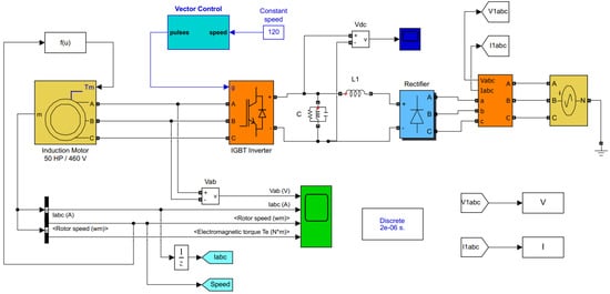
Figure 3.
Simulink model of a composite load.
The model shown was simulated for voltages and frequencies in the 0−550 V and 55−65 Hz range, respectively. The active and reactive powers at the load terminal were computed and recorded for each set of voltages and frequencies. All data points were used in training and validation, as discussed in the next section. A sample of the simulated results is provided in Table 1.

Table 1.
Numerical simulation results—A sample.
Neural networks were used to map the complex and non-linear relationships between the proposed composite load’s active and reactive power consumption and the voltage and frequency of that load. The inputs to the neural networks were the voltage and frequency, and the output was either the active or reactive power consumption of the load. Therefore, two separate neural networks were created based on the same voltage and frequency inputs. The output of the first network was the real power, whereas the second network provided the reactive power as the output. Separate networks were required because of the distinctive characteristics of active and reactive power.
Both neural networks developed as a part of this work consisted of an input layer, a hidden layer, and an output layer. The input layer contained two nodes (V and f), and the hidden layer consisted of several neurons for which the activation function was a hyperbolic tangent sigmoid transfer function. The output layer consisted of one neuron for which the activation function was a pure linear function (purelin). As noted above, the data yielded by the simulation of the implemented Simulink model were used to train and validate the developed neural networks. For this purpose, 250 of 300 data points collected were used to train the neural networks, while the remaining 50 data points were used to test the accuracy of the networks. A back-propagation algorithm was adopted when training the developed neural networks, in which different numbers of hidden neurons were tested. Through trial and error, 75 hidden neurons with suboptimal performance were identified for both neural networks. The first neural network, with active power as the output, required 2305 epochs to reach the desired performance accuracy of a Mean Square Error (MSE) of 0.01, whereas the second neural network required 1255 epochs to reach the same performance accuracy goal of 0.01 MSE. Figure 4 shows the training results for the real-power neural network, while the results for the reactive-power neural network are shown in Figure 5.
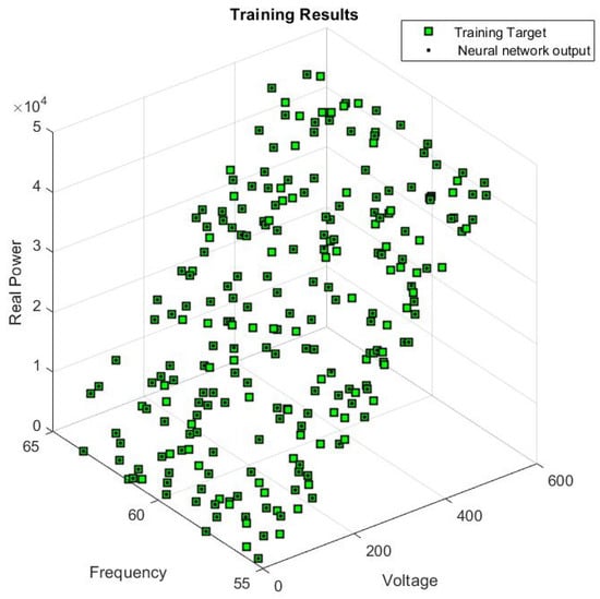
Figure 4.
Training results for real power.
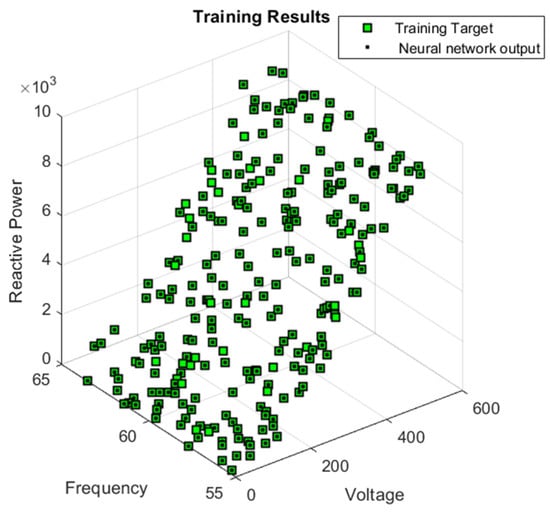
Figure 5.
Training results for reactive power.
After both networks were trained, selected input data were fed into each network. The comparisons between the neural network outputs and the actual output data for real power are shown in Figure 6 and Figure 7, where these are depicted as black dots and green squares, respectively. The neural network for reactive power was also tested after training using 250 data points, as shown in Figure 8 and Figure 9, where the green points represent the target outputs of the tests, and the black points represent the actual outputs of the system.
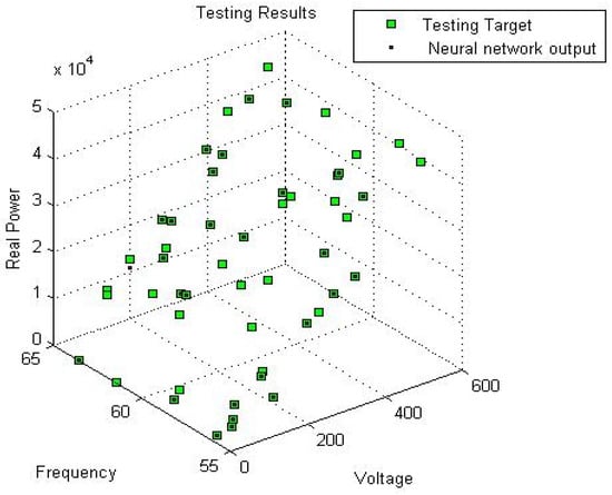
Figure 6.
Test results for real power.
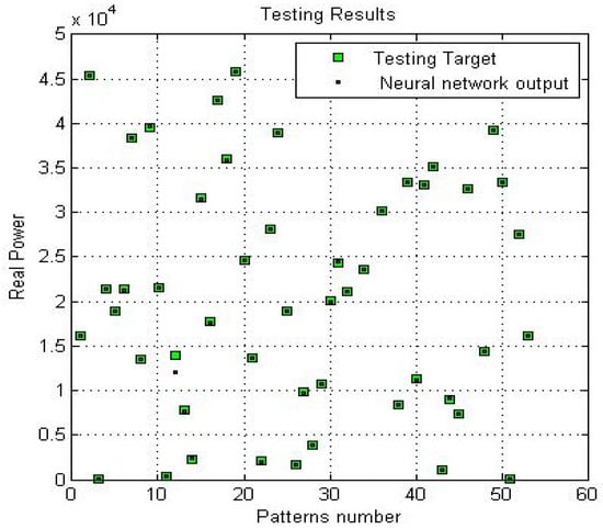
Figure 7.
The results of real power.
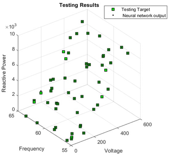
Figure 8.
Test results of reactive power.
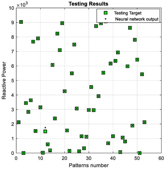
Figure 9.
The results of reactive power.
4. Case Study
To test the effects of different load models on the power system reliability indices, bus 2 of the RBTS [24] was implemented using ETAP software. The RBTS has been referenced for many reliability studies and evaluation techniques in the literature. A description of the bus 2-RBTS and system data can be found in [24,25]. The advantage of the RBTS is the availability of the practical reliability data for all components. Table 2 shows the component types used in the single-line diagram implemented in ETAP.
Table 2.
Number of RBTS Bus 2 components.
A reliability analysis of the implemented power system was performed by considering four scenarios. In the first scenario, all the load points connected to the system are modeled as static loads with constant active and reactive power. In the second scenario, two of the static loads are replaced with induction motors (dynamic loads). For the third scenario, a combination of the two load types is implemented, whereby 11 loads are modeled as static loads and 11 loads are modeled as dynamic loads. In the final scenario, all the load points are modeled as dynamic loads.
The implemented system consisted of four main feeders at a voltage of 11 kV. Each feeder was connected to a different number of loads through a 11/0.4 kV step-down transformer, as shown in Figure 10. Additional information on the parameters pertaining to the cables and transformers incorporated into the implemented power system is shown in Table 3 and Table 4, respectively.
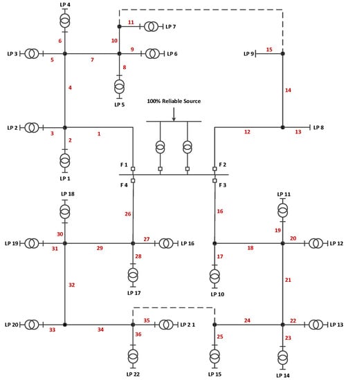
Figure 10.
Single-line diagram of the RBTS bus 2 system.
Table 3.
Cables parameters.
Table 4.
Transformer parameters.
This particular distribution system configuration was considered because, due to the system’s complexity, availabilities of a significant number of components exert a direct effect on its overall reliability. In addition, all customer loads of various load types are connected to the system at the distribution level. For accurate reliability analysis and index calculation, the effects of all components on the availability of the power system must be included because neglecting some aspect of the actual physical behavior of any component in the network will result in underestimating the reliability indices. Traditional reliability indices were used to verify the impact of the load model type on the determined network and customer performance. The failure rate (λ) and repair time for each component are given in Table 5 and were used to calculate the reliability indices for the entire system, namely SAIFI, SAIDI, CAIDI, ASAI, and ENS.
Table 5.
Components failure rate.
Based on the simulation performed using the ETAP software, the reliability indices were calculated for the four load modeling scenarios indicated earlier, with the results displayed in Table 6. For Scenario 1, the system was simulated with all 22 load points modeled as static loads. In Scenario 2, two of the static loads were replaced with induction motors (dynamic loads) and consumed 1.096 MVA at a power factor (pf) of 92.47% and 1.157 MVA at a pf of 92.49%, respectively, thus equaling the power consumption of the replaced static loads. In Scenario 3, 12 of the 22 static loads were replaced with induction motors, six of which consumed 1.096 MVA at a pf of 92.7% while the remaining six consumed 1.157 MVA at a pf of 92.49%. For Scenario 4, all 22 loads were modeled as dynamic loads. The findings confirmed that total power consumption remained constant in all scenarios.
Table 6.
Reliability indices for the system.
Comparison of the indices for all modeled scenarios revealed that the frequency and duration of interruptions per customer in a system with only static loads are lower than those observed in scenarios incorporating dynamic loads. More specifically, a comparison of Scenario 1 with Scenario 4 in which all 22 loads were modeled as dynamic loads reveals that the former not only has a higher overall availability which decreases as more dynamic loads are added, but the energy not served is also lower. These findings can be attributed to the fact that, when only static load modeling is used, the loads are approximated to impose constant active (P) and reactive (Q) power consumption. Thus, the power consumption is not a function of time. However, when a dynamic load such as an induction motor is modeled, the amounts of active and reactive power consumed are functions of time, yielding more accurate and realistic indices with respect to the actual power system loads.
5. Conclusions
The rapid introduction of new load types into power systems necessitates the development of accurate load models using viable load modeling techniques. Such models are desirable because of the need to acquire realistic results in stability studies and reliability analyses. In the present study, a dynamic load model was adopted, and a simulation test bed in MATLAB/Simulink was developed to simulate the model. The simulated data were subsequently used to train and validate a neural network model. Thereafter, a small power system model was established in ETAP using bus 2 of the RBTS, allowing various scenarios to be simulated. As these scenarios consisted of either purely static or dynamic loads at the load points, or a mix of both, the reliability analysis of the SAIDI, SAIFI, CAIDI, ASAI and EENS is more accurate using the proposed load model. The results indicated that these reliability indices are highly sensitive to the manner in which load is represented in modeling. The average frequency and duration of interruptions were found to be underestimated when static load models were used. The energy not supplied increased considerably when dynamic rather than static load models were employed in the reliability assessment. Therefore, considering the increasing prevalence of non-linear and complex loads, it is necessary to adopt accurate and suitable load models in reliability calculations to minimize inaccuracy of calculated reliability indices.
Author Contributions
Conceptualization, L.M. and M.A.; methodology, L.M. and M.A.; software, L.M. and M.H.; validation, M.A. and M.K.; formal analysis, L.M. and M.A.; investigation, L.M. and M.A.; resources, L.M. and M.K.; data curation, M.H.; writing—original draft preparation, L.M.; M.A.; M.K. and M.H.; writing—review and editing, M.A. and M.K.; visualization, L.M. and M.A.; supervision, M.A.; All authors have read and agreed to the published version of the manuscript.
Funding
This research received no external funding.
Institutional Review Board Statement
Not applicable.
Informed Consent Statement
Not applicable.
Data Availability Statement
Not applicable.
Acknowledgments
This work was supported by the King Fahd University of Petroleum and Minerals (KFUPM), Dhahran, Saudi Arabia.
Conflicts of Interest
The authors declare no conflict of interest.
References
- Taylor, C. Power System Voltage Stability; McGraw-Hill: New York, NY, USA, 1994. [Google Scholar]
- Mitra, A.; Dutta, R.; Gupta, A.; Mohapatra, A.; Chakrabarti, S. A robust data-driven approach for adaptive dynamic load modeling. IEEE Trans. Power Syst. 2022, 37, 3779–3791. [Google Scholar] [CrossRef]
- Paidi, E.; Nechifor, A.; Albu, M.; Yu, J.; Terzija, V. Development and validation of a new oscillatory component load model for real-time estimation of dynamic load model parameters. IEEE Trans. Power Deliv. 2020, 35, 618–629. [Google Scholar] [CrossRef]
- Wang, X.; Wang, Y.; Shi, D.; Wang, J.; Wang, Z. Two-stage WECC composite load modeling: A double deep q-learning networks approach. IEEE Trans. Smart Grid 2020, 11, 4331–4344. [Google Scholar] [CrossRef]
- Chávarro-Barrera, L.; Pérez-Londoño, S.; Mora-Flórez, J. An adaptive approach for dynamic load modeling in microgrids. IEEE Trans. Smart Grid 2021, 12, 2834–2843. [Google Scholar] [CrossRef]
- Wang, S.; Huang, R.; Huang, Z.; Fan, R. A robust dynamic state estimation approach against model errors caused by load changes. IEEE Trans. Power Syst. 2020, 35, 4518–4527. [Google Scholar] [CrossRef]
- Keyhani, A.; Lu, W.; Heydt, G.T. Neural Network Based Composite Load Models for Power System Stability Analysis. In Proceedings of the 2005 IEEE International Conference on Computational Intelligence for Measurement Systems and Applications, Messian, Italy, 20–22 July 2005. [Google Scholar]
- Karki, R.; Billinton, R.; Verma, A. Reliability Modeling and Analysis of Smart Power Systems; Springer: Berlin/Heidelberg, Germany, 2014. [Google Scholar]
- Veliz, F.; Borges, C.; Rei, A. A comparison of load models for composite reliability evaluation by nonsequential monte carlo simulation. IEEE Trans. Power Syst. 2010, 25, 649–656. [Google Scholar] [CrossRef]
- Cho, N.; Awodele, K. Comparison of Four Load Models for Reliability Evaluation Considering Reconfiguration Using Monte Carlo Simulation. In Proceedings of the 2012 IEEE International Conference on Power System Technology (POWERCON), Auckland, New Zealand, 30 October–2 November 2012. [Google Scholar] [CrossRef]
- Wong, K.; Haque, M. Dynamic load modelling of a paper mill for small signal stability studies. IET Gener. Transm. Distrib. 2014, 8, 131–141. [Google Scholar] [CrossRef]
- Navarro, I. Dynamic Load Models for Power Systems-Estimation of Time-Varying Parameters during Normal Operation; Department of Industrial Electrical Engineering and Automation, Lund Institute of Technology: Lund, Sweden, 2002. [Google Scholar]
- Collin, A.; Acosta, J.; Hayes, B.; Djokic, S. Component-Based Aggregate Load Models for Combined Power Flow and Harmonic Analysis. In Proceedings of the 7th Mediterranean Conference and Exhibition on Power Generation, Transmission, Distribution and Energy Conversion (MedPower 2010), Agia Napa, Cyprus, 7–10 November 2010. [Google Scholar] [CrossRef]
- Chassin, F.; Mayhorn, E.; Elizondo, M.; Lu, S. Load Modeling and Calibration Techniques for Power System Studies. In Proceedings of the 2011 North American Power Symposium, Boston, MA, USA, 4–6 August 2011. [Google Scholar] [CrossRef]
- Morison, K.; Hamadani, H.; Wang, L. Load Modeling for Voltage Stability Studies. In Proceedings of the 2006 IEEE PES Power Systems Conference and Exposition, Atlanta, GA, USA, 29 October–1 November 2006. [Google Scholar] [CrossRef]
- Hajagos, L.; Danai, B. Laboratory measurements and models of modern loads and their effect on voltage stability studies. IEEE Trans. Power Syst. 1998, 13, 584–592. [Google Scholar] [CrossRef]
- Price, W.W.; Taylor, C.W.; Rogers, G.J. Standard load models for power flow and dynamic performance simulation. IEEE Trans. Power Syst. 1995, 10, 1302–1313. [Google Scholar] [CrossRef]
- Ju, P.; Shi, K.; Tang, Y.; Shao, Z.; Chen, Q.; Yang, W. Comparisons between the Load Models with Considering Distribution Network Directly or Indirectly. In Proceedings of the 2008 Joint International Conference on Power System Technology and IEEE Power India Conference, New Delhi, India, 12–15 October 2008. [Google Scholar] [CrossRef]
- Zhang, J.; Yan, A.; Chen, Z.; Gao, K. Dynamic synthesis load modeling approach based on load survey and load curves analysis. In Proceedings of the 2008 Third International Conference on Electric Utility Deregulation and Restructuring and Power Technologies, Nanjing, China, 6–9 April 2008. [Google Scholar] [CrossRef]
- Lin, C.J.; Chen, A.T.; Chiou, C.Y.; Huang, C.H.; Chiang, H.D.; Wang, J.C.; Fekih-Ahmed, L. Dynamic load models in power systems using the measurement approach. IEEE Trans. Power Syst. 1993, 8, 309–315. [Google Scholar] [CrossRef]
- Knyazkin, V.; Canizares, C.; Soder, L. On the parameter estimation and modeling of aggregate power system loads. IEEE Trans. Power Syst. 2004, 19, 1023–1031. [Google Scholar] [CrossRef]
- Price, W.W.; Wirgau, K.A.; Murdoch, A.; Mitsche, J.V.; Vaahedi, E.; El-Kady, M. Load modelling for power flow and transient stability computer studies. IEEE Trans. Power Syst. 1998, 3, 180–187. [Google Scholar] [CrossRef]
- Bostanci, M.; Koplowitz, J.; Taylor, C. Identification of power system load dynamics using artificial neural networks. IEEE Trans. Power Syst. 1997, 12, 1468–1473. [Google Scholar] [CrossRef]
- Billinton, R.; Kumar, S.; Chowdhury, N.; Chu, K.; Debnath, K.; Goel, L.; Khan, E.; Kos, P.; Nourbakhsh, G.; Oteng-Adjei, J. A reliability test system for educational purposes-basic data. IEEE Power Eng. Rev. 1989, 9, 67–68. [Google Scholar] [CrossRef]
- Allan, R.N.; Billinton, R.; Sjarief, I.; Goel, L.; So, K.S. Reliability test system for education purposes—Basic distribution system data and results. IEEE Trans. Power Syst. 1991, 6, 813–820. [Google Scholar] [CrossRef]


Disclaimer/Publisher’s Note: The statements, opinions and data contained in all publications are solely those of the individual author(s) and contributor(s) and not of MDPI and/or the editor(s). MDPI and/or the editor(s) disclaim responsibility for any injury to people or property resulting from any ideas, methods, instructions or products referred to in the content. |
© 2023 by the authors. Licensee MDPI, Basel, Switzerland. This article is an open access article distributed under the terms and conditions of the Creative Commons Attribution (CC BY) license (https://creativecommons.org/licenses/by/4.0/).