
A Hybrid Time Series Model for Predicting the Displacement of High Slope in the Loess Plateau Region

Abstract
:
1. Introduction
2. Methodology
2.1. Support Vector Machine (SVM)
2.2. Long Short-Term Memory Network (LSTM)
2.3. Optimization of the Prediction Models
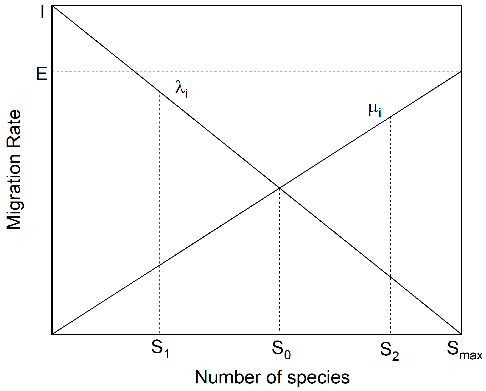
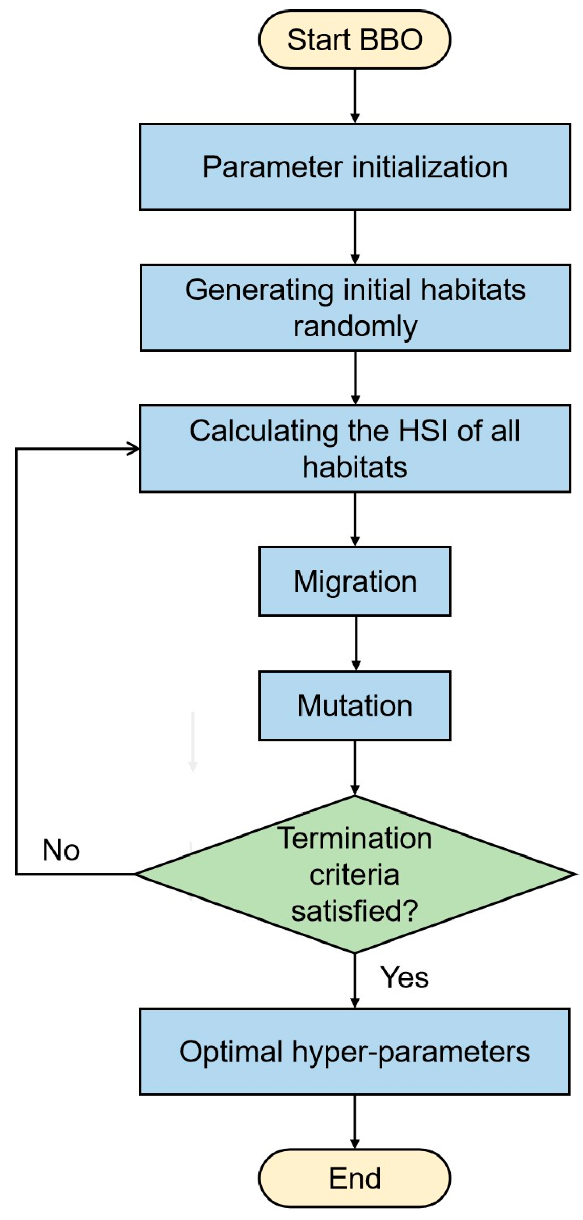
2.3.1. Hyperparameter Optimization Using BBO
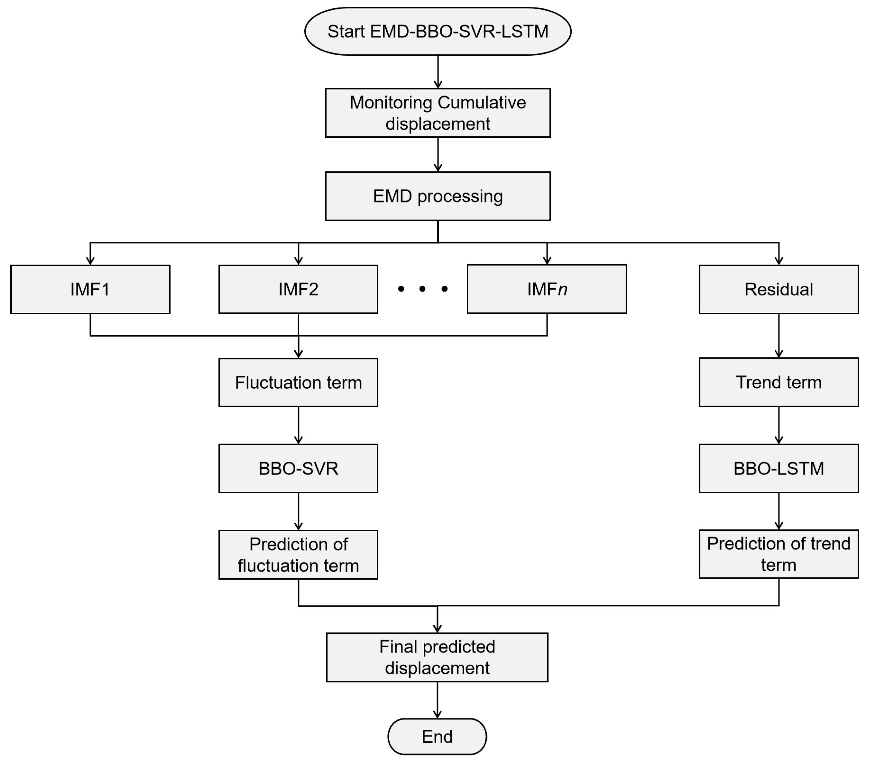
2.3.2. EMD-BBO-SVR-LSTM
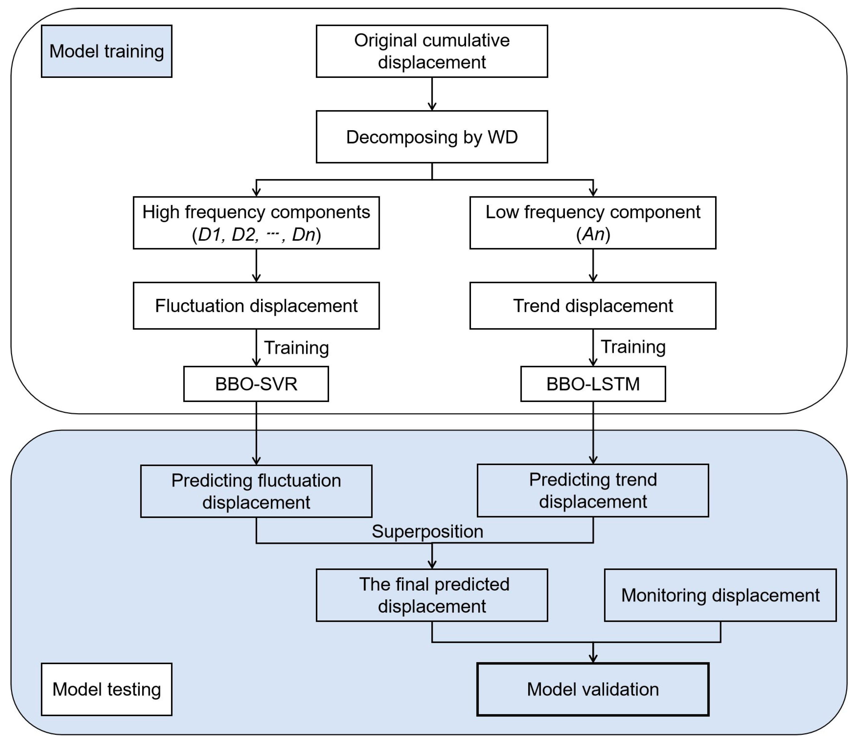
2.3.3. WD-BBO-SVR-LSTM
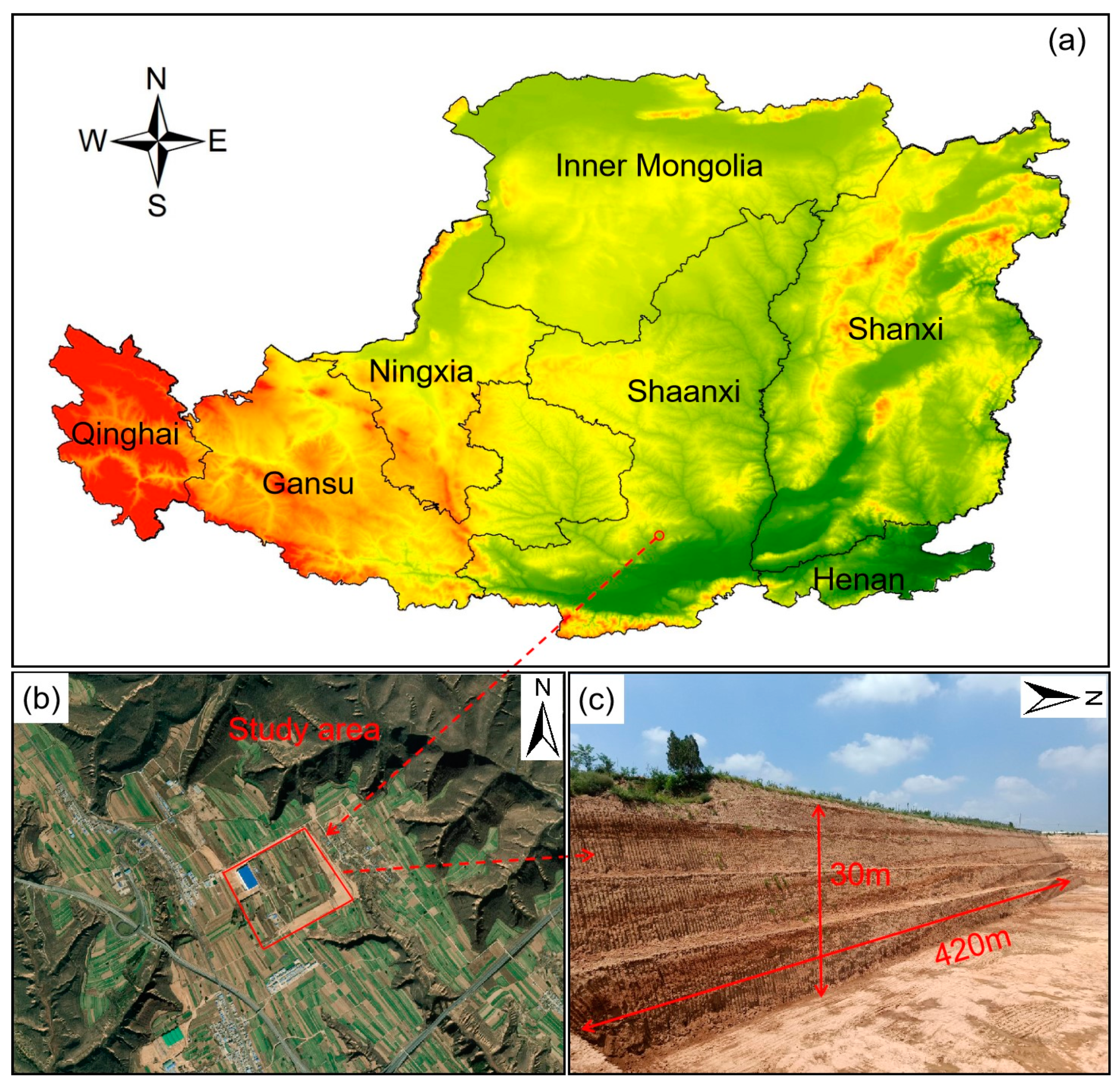
3. A Case Study of a Loess Slope in China
3.1. Introduction of the Slope Case
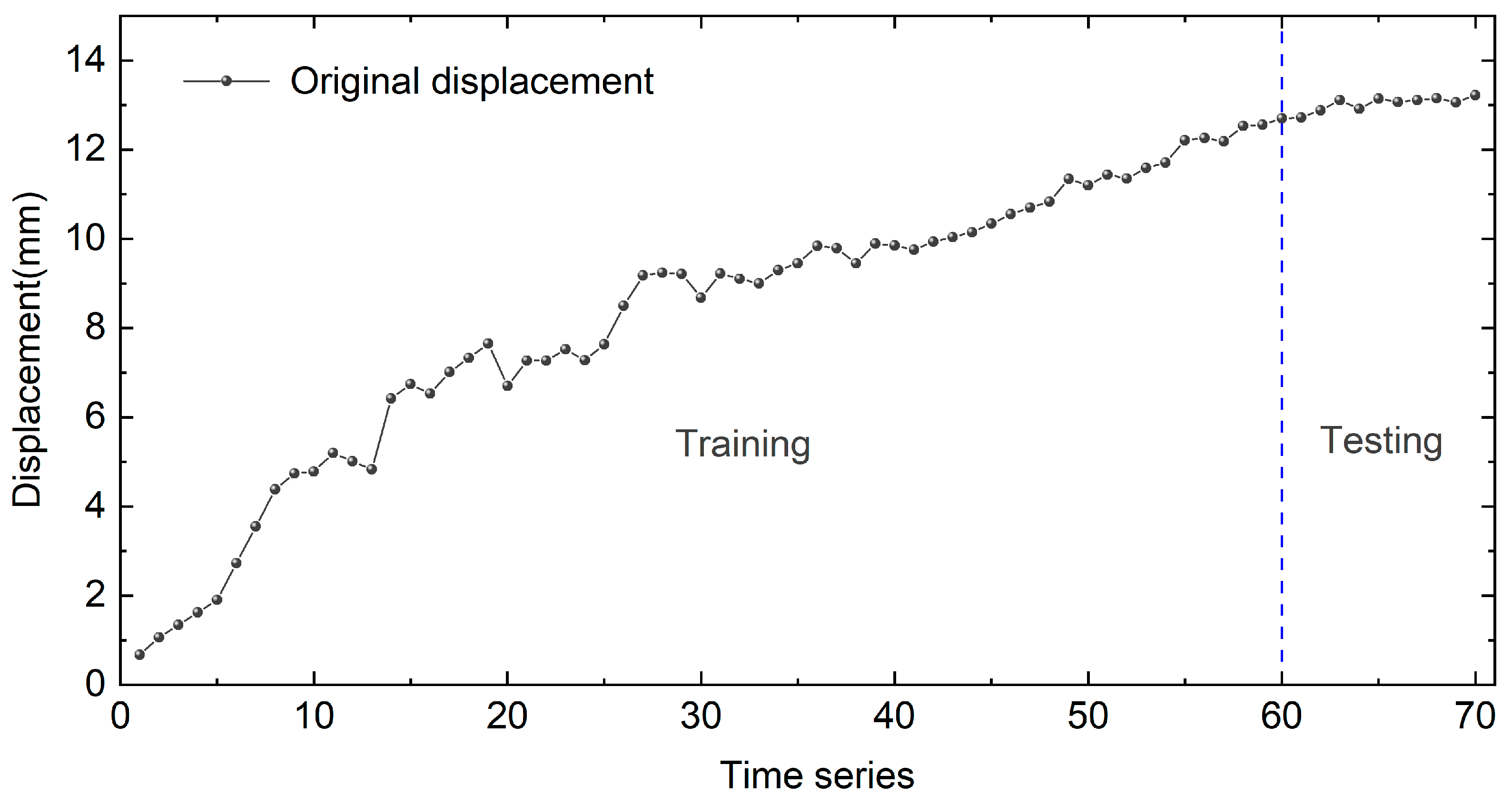
3.2. Data Preparation and Evaluation Indices
4. Results and Discussion
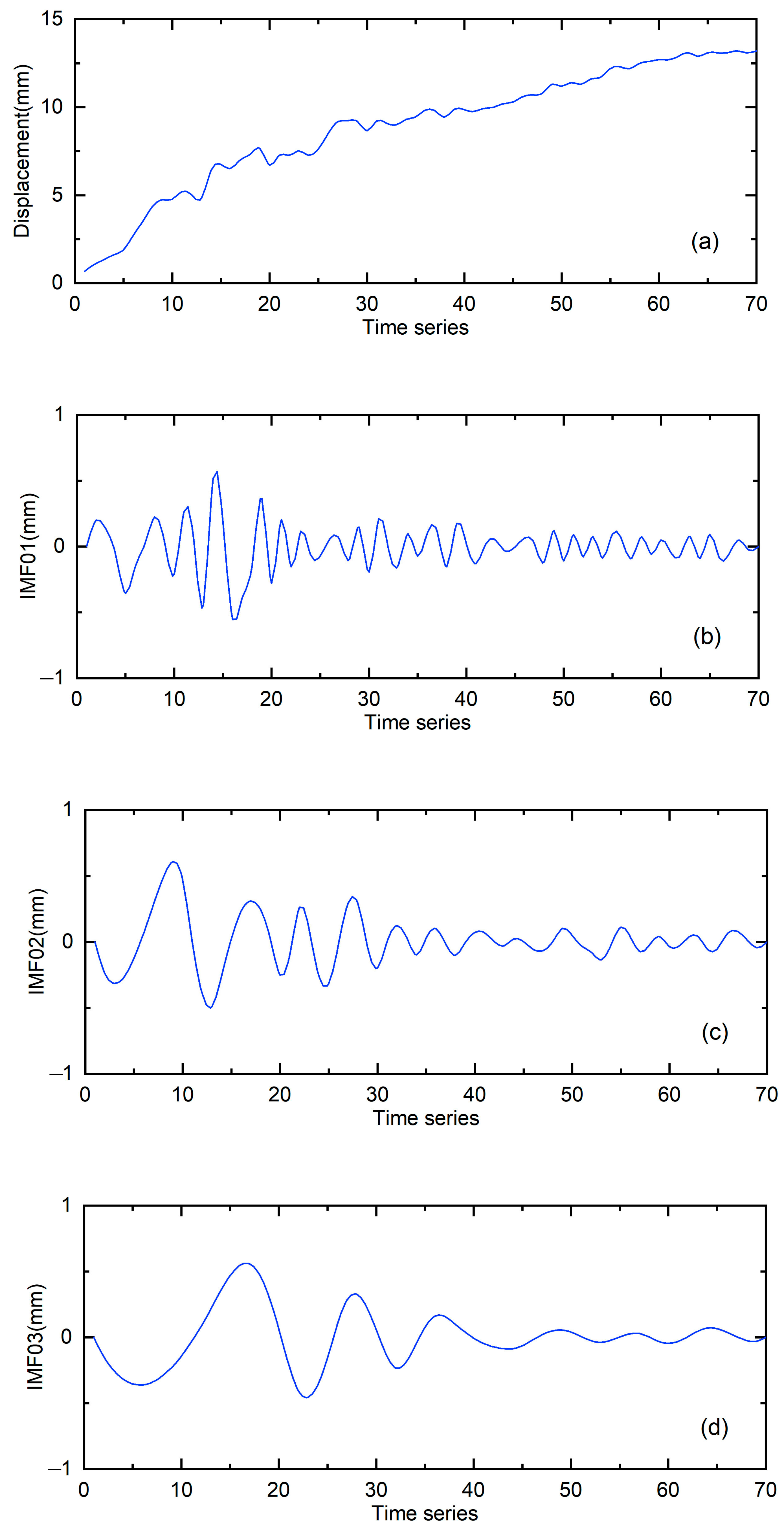
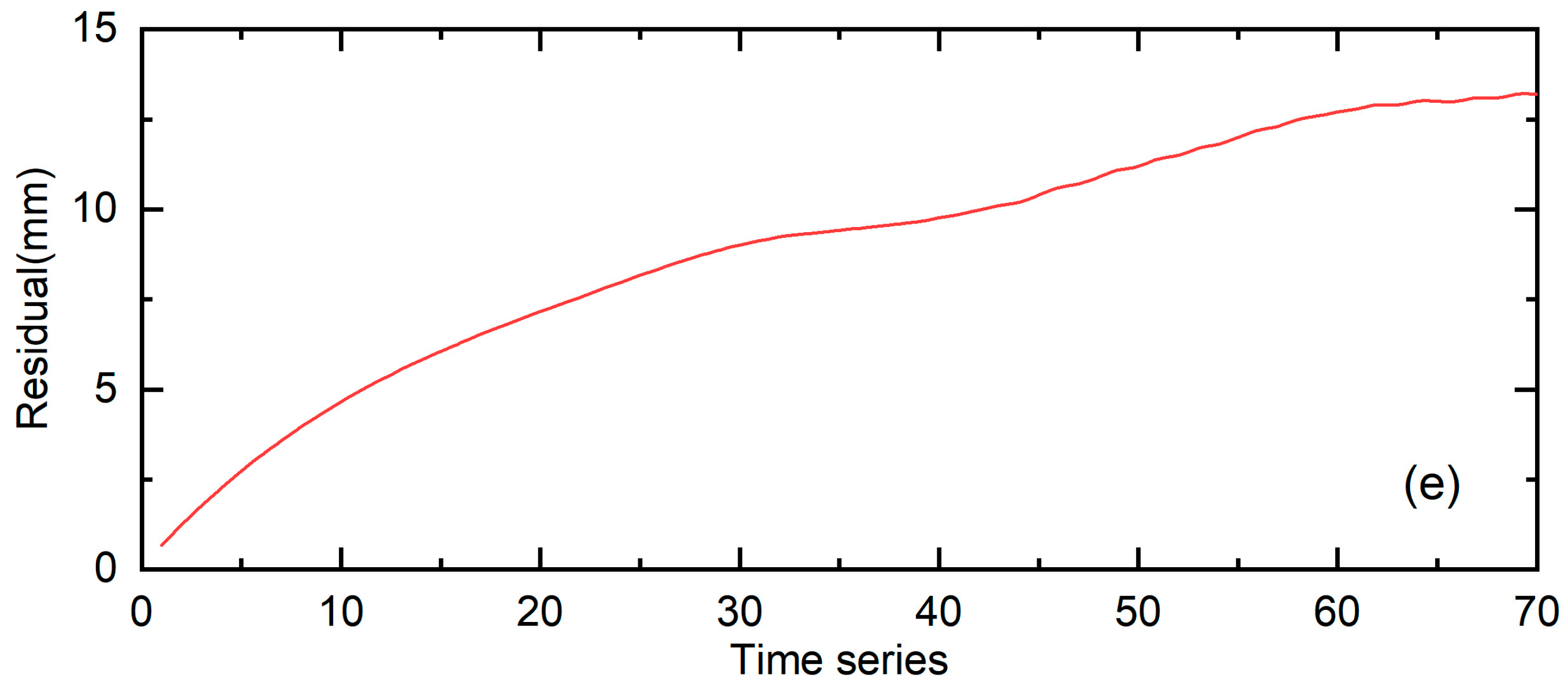
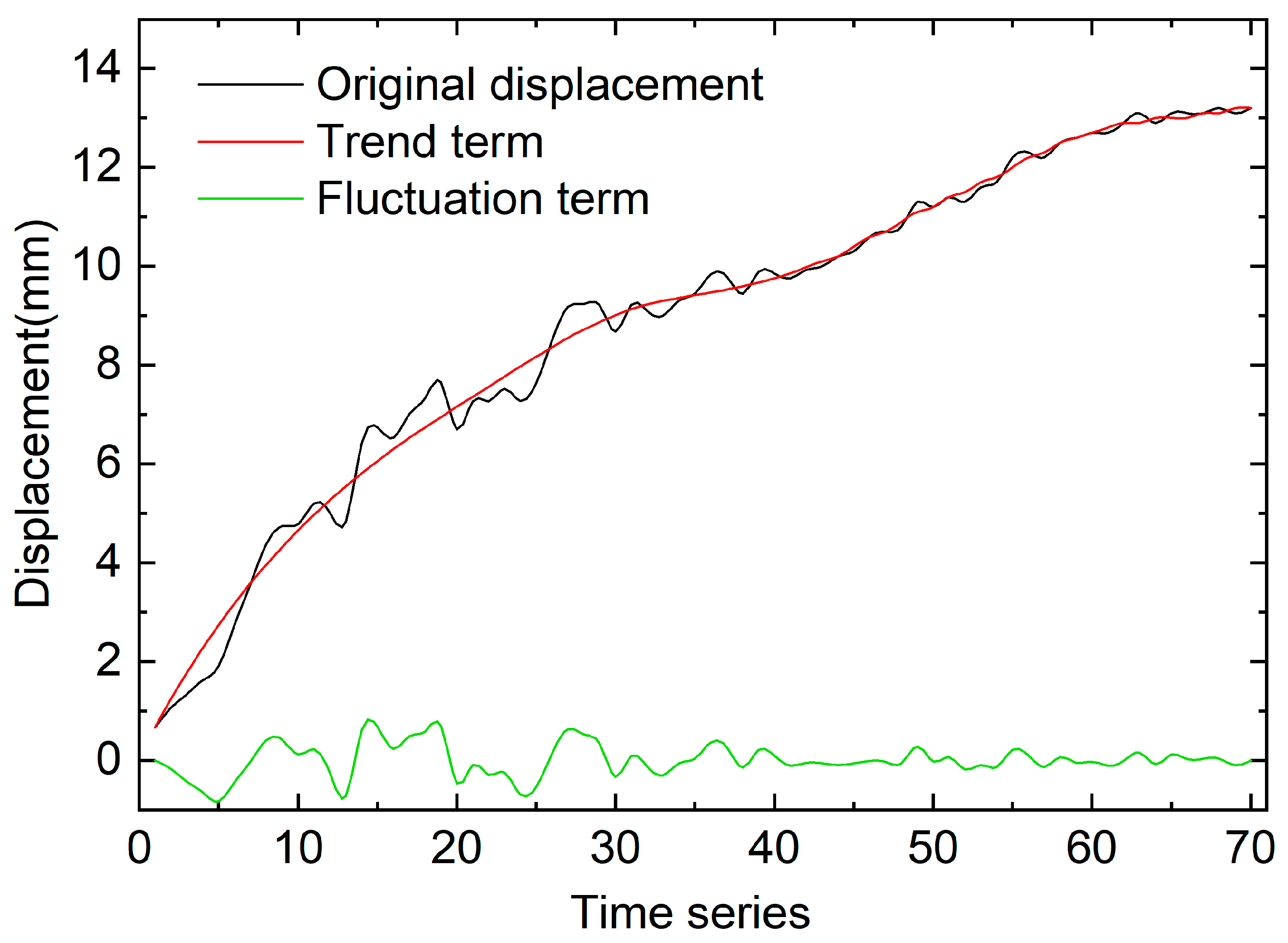
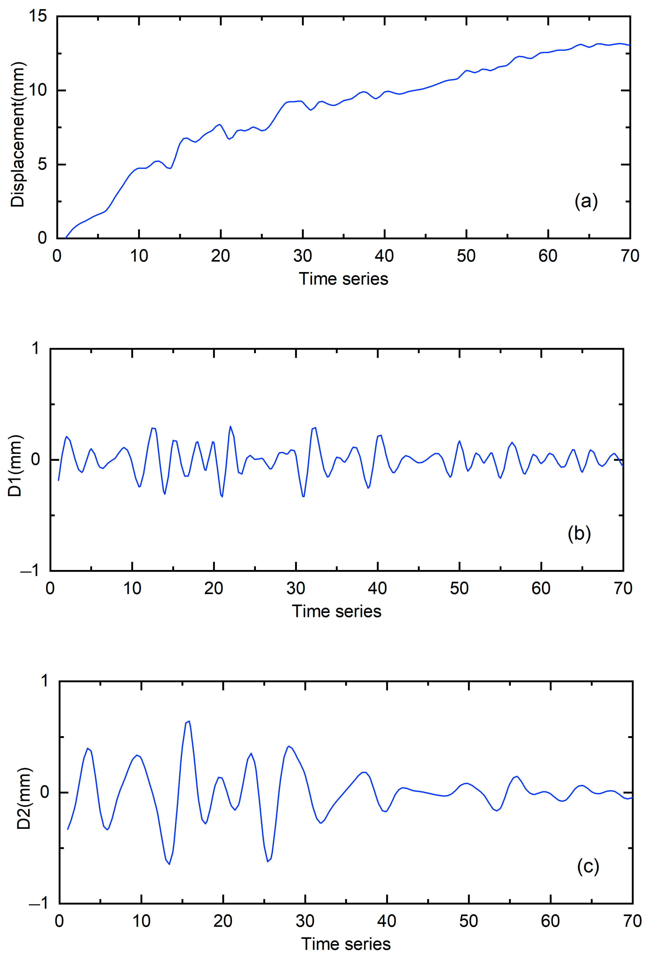
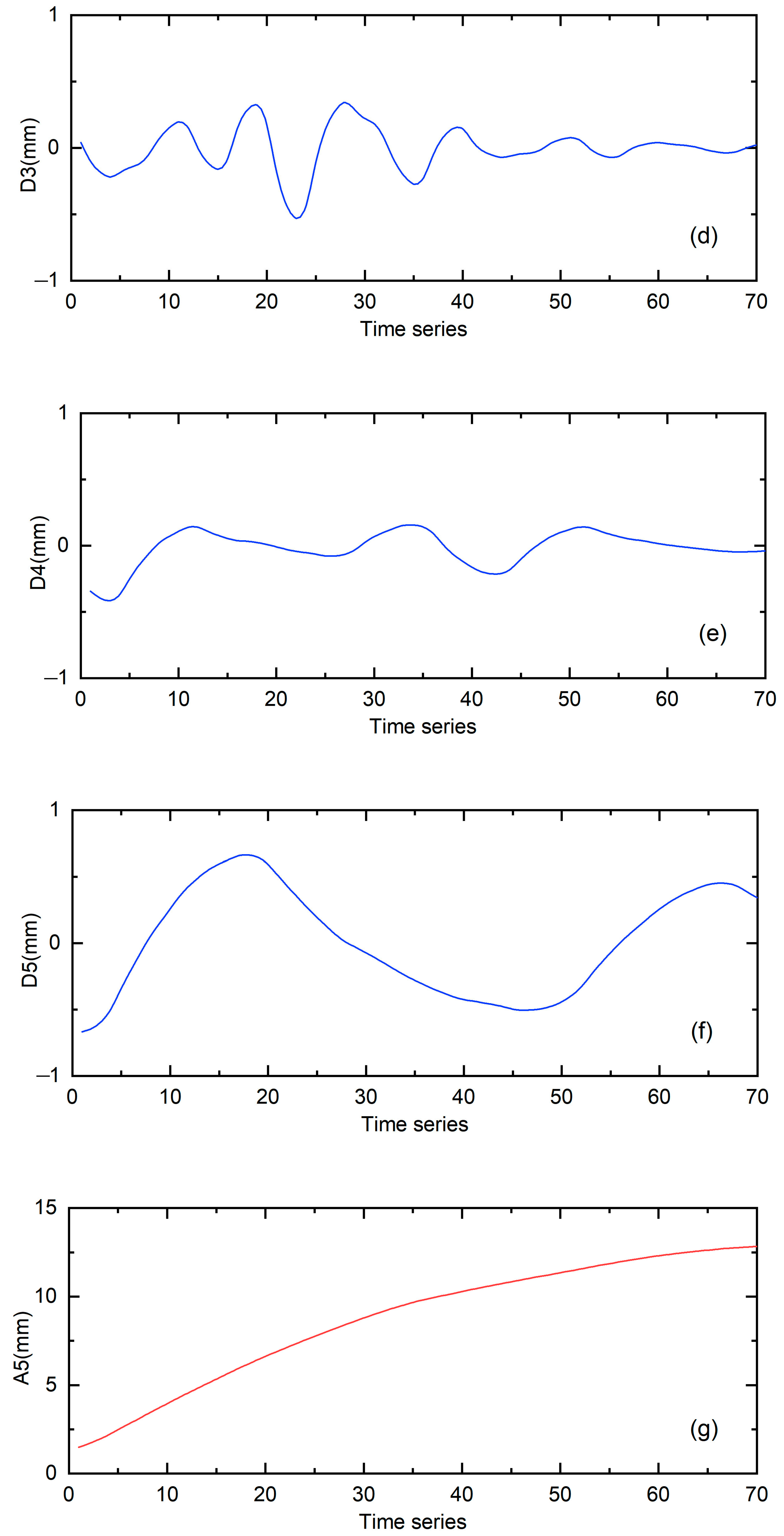
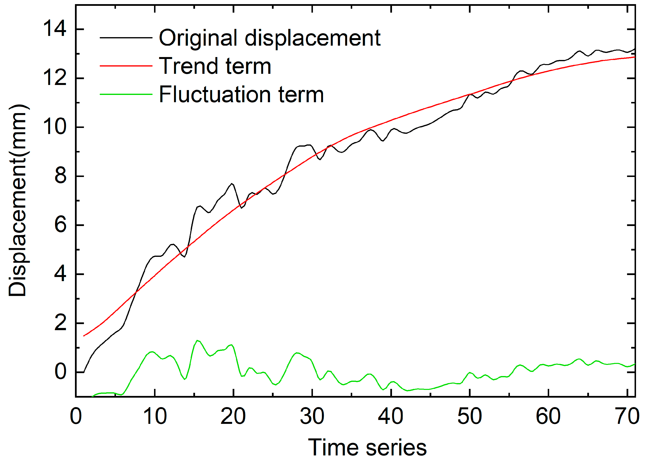
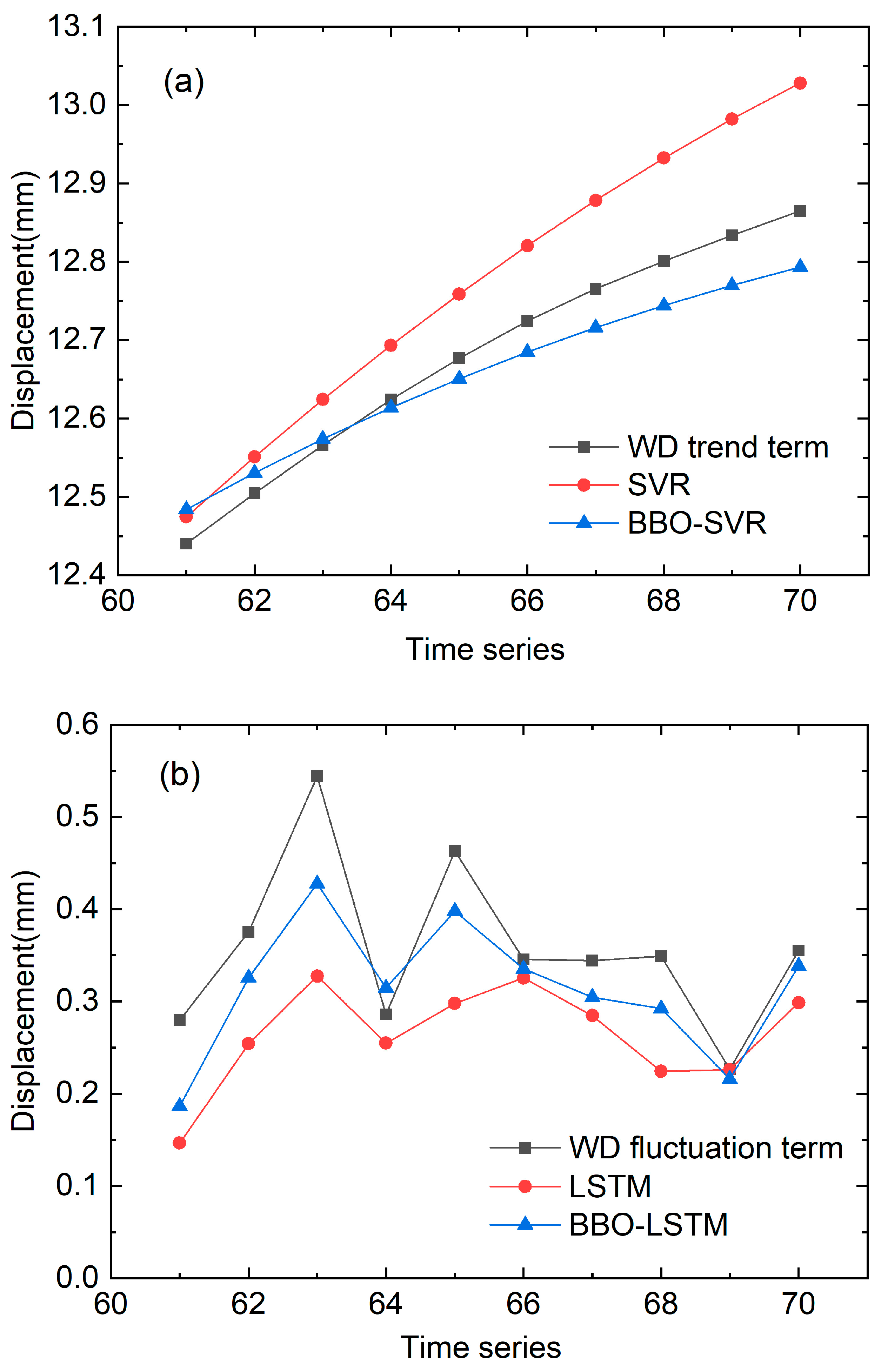
4.1. The Decomposition of the Slope Displacement by EMD and WD
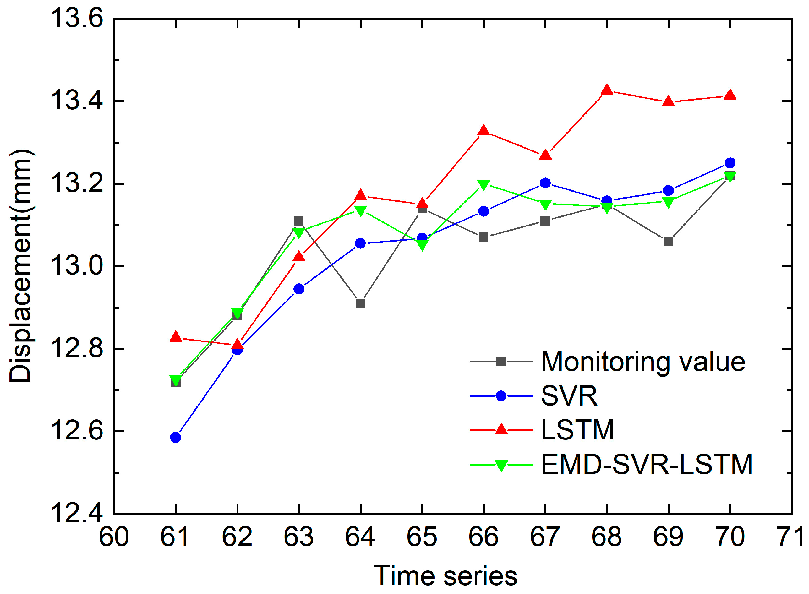
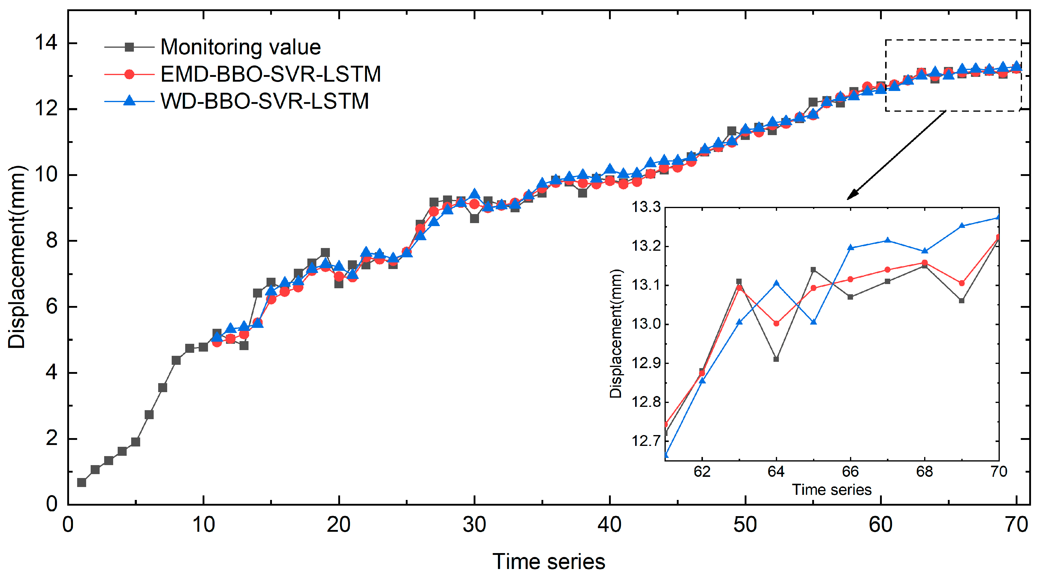
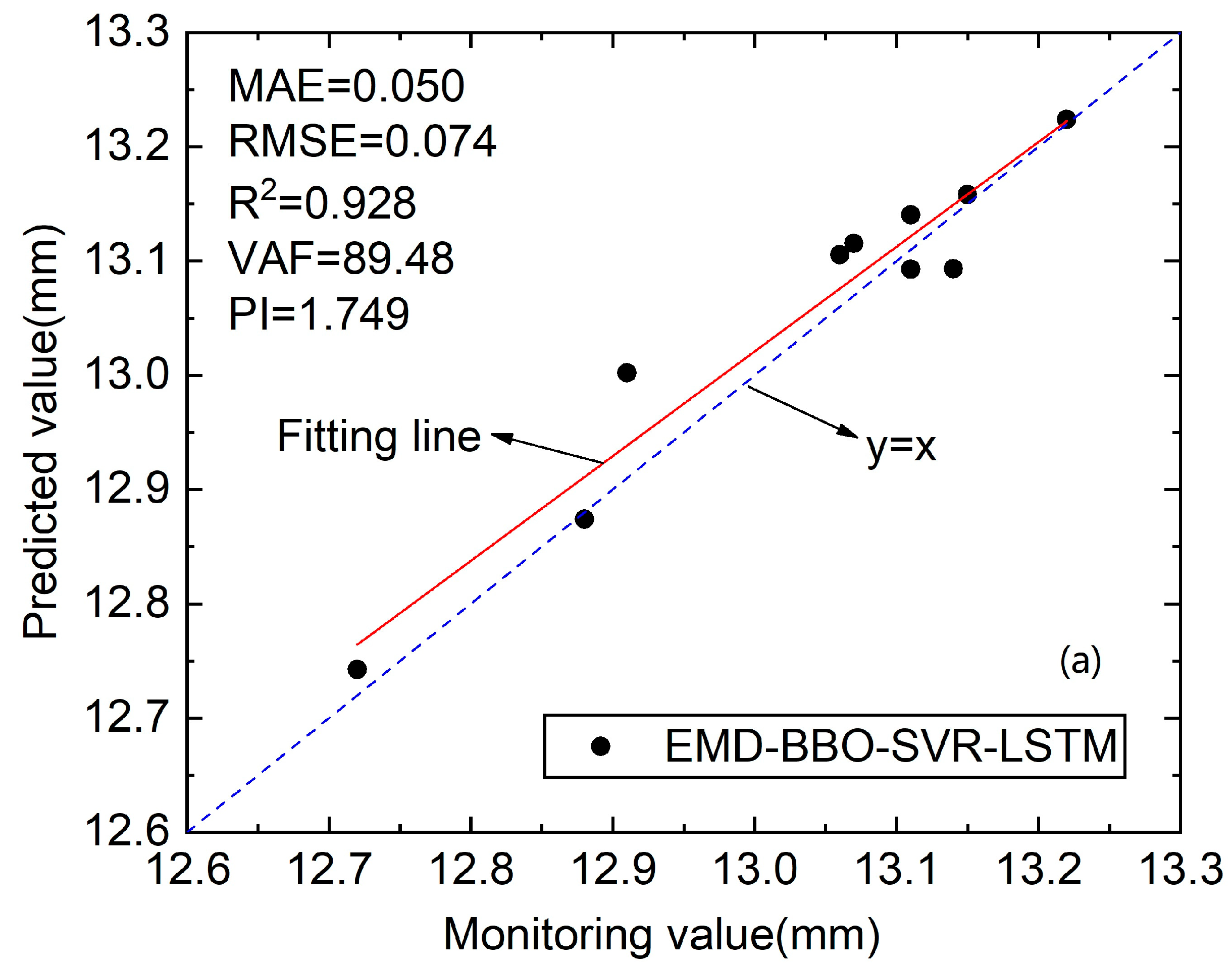
4.2. Comparison of Prediction Results
5. Conclusions
Author Contributions
Funding
Institutional Review Board Statement
Informed Consent Statement
Data Availability Statement
Conflicts of Interest
References
- Chang, C.; Bo, J.; Qi, W.; Qiao, F.; Peng, D. Study on instability and damage of a loess slope under strong ground motion by numerical simulation. Soil Dyn. Earthq. Eng. 2022, 152, 107050. [Google Scholar] [CrossRef]
- Chang, Z.; Huang, F.; Huang, J.; Jiang, S.-H.; Zhou, C.; Zhu, L. Experimental study of the failure mode and mechanism of loess fill slopes induced by rainfall. Eng. Geol. 2021, 280, 105941. [Google Scholar] [CrossRef]
- Li, H.; Du, Q.-W. Stabilizing a post-landslide loess slope with anti-slide piles in Yanan, China. Environ. Earth Sci. 2021, 80, 739. [Google Scholar] [CrossRef]
- Singh, P.; Bardhan, A.; Han, F.; Samui, P.; Zhang, W. A critical review of conventional and soft computing methods for slope stability analysis. Model. Earth Syst. Environ. 2023, 9, 1–17. [Google Scholar] [CrossRef]
- Sun, Y.; Jiang, Q.; Yin, T.; Zhou, C. A back-analysis method using an intelligent multi-objective optimization for predicting slope deformation induced by excavation. Eng. Geol. 2018, 239, 214–228. [Google Scholar] [CrossRef]
- Bharti, J.P.; Mishra, P.; Moorthy, U.; Sathishkumar, V.E.; Cho, Y.; Samui, P. Slope Stability Analysis Using Rf, Gbm, Cart, Bt and Xgboost. Geotech. Geol. Eng. 2021, 39, 3741–3752. [Google Scholar] [CrossRef]
- Samui, P. Slope stability analysis: A support vector machine approach. Environ. Geol. 2008, 56, 255–267. [Google Scholar] [CrossRef]
- Saito, M. Forecasting time of slope failure by tertiary creep. In Proceedings of the 7th International Conference on Soil Mechanics and Foundation Engineering, Mexico City, Mexico, 29 August 1969; pp. 677–683. [Google Scholar]
- Hoek, E.; Bray, J.D. Rock Slope Engineering; CRC Press: Boca Raton, FL, USA, 1981. [Google Scholar]
- Hayashi, S.; Yamamori, T. Basic Equation of Slide in Tertiary Creep and Features of its Parameters. Landslides 1991, 28, 17–22. [Google Scholar] [CrossRef] [Green Version]
- Stevenson, P.C. An empirical method for the evaluation of relative landslip risk. Bull. Int. Assoc. Eng. Geol.-Bull. L’association Int. Géologie L’ingénieur 1977, 16, 69–72. [Google Scholar] [CrossRef]
- Federico, A.; Popescu, M.; Fidelibus, C.; Internò, G. On the prediction of the time of occurrence of a slope failure: A review. In Landslides: Evaluation and Stabilization/Glissement de Terrain: Evaluation et Stabilisation, Set of 2 Volumes; CRC: Boca Raton, FL, USA, 2004; pp. 979–983. [Google Scholar] [CrossRef]
- Miao, S.; Hao, X.; Guo, X.; Wang, Z.; Liang, M. Displacement and landslide forecast based on an improved version of Saito’s method together with the Verhulst-Grey model. Arab. J. Geosci. 2017, 10, 53. [Google Scholar] [CrossRef]
- Rice, R.; Pillsbury, N. Predicting landslides in clearcut patches. In Recent Developments in the Explanation and Prediction of Erosion and Sediment Yield, Proceedings of the Exeter Symposium, Exeter, UK, 19–30 July 1982; International Association of Hydrological Sciences Wallingford: Oxfordshire, UK, 1982. [Google Scholar]
- Li, X.; Kong, J.; Wang, Z. Landslide displacement prediction based on combining method with optimal weight. Nat. Hazards 2012, 61, 635–646. [Google Scholar] [CrossRef]
- Liu, Z.; Xu, W.; Meng, Y.; Chen, H. Modification of GM (1, 1) and its application in analysis of rock-slope deformation. In Proceedings of the 2009 IEEE International Conference on Grey Systems and Intelligent Services (GSIS 2009), Nanjing, China, 10–12 November 2009; pp. 415–419. [Google Scholar] [CrossRef]
- Hayashi, S.; Park, B.-W.; Komamura, F.; Yamamori, T. On the Forecast of Time to Failure of Slope (II) Approximate Forecast in the Early Period of the Tertiary Creep. Landslides 1988, 25, 11–16_1. [Google Scholar] [CrossRef]
- Bhatawdekar, R.M.; Raina, A.K.; Jahed Armaghani, D. A Comprehensive Review of Rockmass Classification Systems for Assessing Blastability. In Proceedings of Geotechnical Challenges in Mining, Tunneling and Underground Infrastructures; Springer Nature: Singapore, 2022; pp. 563–578. [Google Scholar] [CrossRef]
- Samui, P. 14—Slope Stability Analysis Using Multivariate Adaptive Regression Spline. In Metaheuristics in Water, Geotechnical and Transport Engineering; Elsevier: Oxford, UK, 2013; pp. 327–342. [Google Scholar] [CrossRef]
- Bhatawdekar, R.M.; Edy, M.T.; Danial, J.A. Building Information Model for Drilling and Blasting for Tropically Weathered Rock. J. Mines Met. Fuels 2022, 67, 494–500. [Google Scholar]
- Huang, F.; Yin, K.; Zhang, G.; Gui, L.; Yang, B.; Liu, L. Landslide displacement prediction using discrete wavelet transform and extreme learning machine based on chaos theory. Environ. Earth Sci. 2016, 75, 1376. [Google Scholar] [CrossRef]
- Murlidhar, B.R.; Ahmed, M.; Mavaluru, D.; Siddiqi, A.F.; Mohamad, E.T. Prediction of rock interlocking by developing two hybrid models based on GA and fuzzy system. Eng. Comput. 2019, 35, 1419–1430. [Google Scholar] [CrossRef]
- Wan, D.; Wang, M.; Zhu, Z.; Wang, F.; Zhou, L.; Liu, R.; Gao, W.; Shu, Y.; Xiao, H. Coupled GIMP and CPDI material point method in modelling blast-induced three-dimensional rock fracture. Int. J. Min. Sci. Technol. 2022, 32, 1097–1114. [Google Scholar] [CrossRef]
- Wang, Z.; Wang, M.; Zhou, L.; Zhu, Z.; Shu, Y.; Peng, T. Research on uniaxial compression strength and failure properties of stratified rock mass. Theor. Appl. Fract. Mech. 2022, 121, 103499. [Google Scholar] [CrossRef]
- Gade, M.; Nayek, P.S.; Dhanya, J. A new neural network–based prediction model for Newmark’s sliding displacements. Bull. Eng. Geol. Environ. 2021, 80, 385–397. [Google Scholar] [CrossRef]
- Liu, K.; Qiao, C.; Teng, W. Research on non-linear time sequence intelligent model construction and prediction of slope displacement by using support vector machine algorithm. Chin. J. Geotech. Eng. 2004, 26, 57–61. [Google Scholar] [CrossRef]
- Liu, C.; Jiang, Z.; Han, X.; Zhou, W. Slope displacement prediction using sequential intelligent computing algorithms. Measurement 2019, 134, 634–648. [Google Scholar] [CrossRef]
- Cai, Z.; Xu, W.; Meng, Y.; Shi, C.; Wang, R. Prediction of landslide displacement based on GA-LSSVM with multiple factors. Bull. Eng. Geol. Environ. 2016, 75, 637–646. [Google Scholar] [CrossRef]
- Du, J.; Yin, K.; Lacasse, S. Displacement prediction in colluvial landslides, Three Gorges Reservoir, China. Landslides 2013, 10, 203–218. [Google Scholar] [CrossRef]
- Zhang, J.; Yin, K.; Wang, J.; Huang, F. Displacement prediction of Baishuihe landslide based on time series and PSO-SVR model. Chin. J. Rock Mech. Eng. 2015, 2, 10. [Google Scholar] [CrossRef]
- Zhang, J.; Peng, T.; Mo, L.; Hu, X.; Wang, X. Research on Highway Slope Monitoring Data Prediction Based on Long Short-term Memory Network. IOP Conf. Ser. Earth Environ. Sci. 2020, 571, 012087. [Google Scholar] [CrossRef]
- Xie, P.; Zhou, A.; Chai, B. The Application of Long Short-Term Memory(LSTM) Method on Displacement Prediction of Multifactor-Induced Landslides. IEEE Access 2019, 7, 54305–54311. [Google Scholar] [CrossRef]
- Tang, Y.; Feng, F.; Guo, Z.; Feng, W.; Li, Z.; Wang, J.; Sun, Q.; Ma, H.; Li, Y. Integrating principal component analysis with statistically-based models for analysis of causal factors and landslide susceptibility mapping: A comparative study from the loess plateau area in Shanxi (China). J. Clean. Prod. 2020, 277, 124159. [Google Scholar] [CrossRef]
- Zhang, Y.-g.; Tang, J.; He, Z.-y.; Tan, J.; Li, C. A novel displacement prediction method using gated recurrent unit model with time series analysis in the Erdaohe landslide. Nat. Hazards 2021, 105, 783–813. [Google Scholar] [CrossRef]
- Duan, W.Y.; Han, Y.; Huang, L.M.; Zhao, B.B.; Wang, M.H. A hybrid EMD-SVR model for the short-term prediction of significant wave height. Ocean Eng. 2016, 124, 54–73. [Google Scholar] [CrossRef]
- Xu, S.; Niu, R. Displacement prediction of Baijiabao landslide based on empirical mode decomposition and long short-term memory neural network in Three Gorges area, China. Comput. Geosci.-UK 2018, 111, 87–96. [Google Scholar] [CrossRef]
- Liu, Z.-q.; Guo, D.; Lacasse, S.; Li, J.-h.; Yang, B.-b.; Choi, J.-c. Algorithms for intelligent prediction of landslide displacements. J. Zhejiang Univ. A 2020, 21, 412–429. [Google Scholar] [CrossRef]
- Vapnik, V.N. Statistical Learning Theory; John Wiley & Sons: New York, NY, USA, 1998. [Google Scholar]
- Vapnik, V.N. The Nature of Statistical Learning Theory; Springer: New York, NY, USA, 2000. [Google Scholar]
- Smola, A.J.; Schölkopf, B. A tutorial on support vector regression. Stat. Comput. 2004, 14, 199–222. [Google Scholar] [CrossRef] [Green Version]
- Wei, C.; Jianli, X.; Liu, Y. Speed estimation based on multiple kernel learning. In Proceedings of the 2012 12th International Conference on ITS Telecommunications, Taipei, Taiwan, 5–8 November 2012; pp. 24–28. [Google Scholar] [CrossRef]
- Wu, C.-H.; Wei, C.-C.; Su, D.-C.; Chang, M.-H.; Ho, J.-M. Travel time prediction with support vector regression. In Proceedings of the 2003 IEEE International Conference on Intelligent Transportation Systems, Shanghai, China, 12–15 October 2003; Volume 2, pp. 1438–1442. [Google Scholar] [CrossRef] [Green Version]
- Hochreiter, S.; Schmidhuber, J. Long Short-Term Memory. Neural Comput. 1997, 9, 1735–1780. [Google Scholar] [CrossRef]
- Ding, N.; Li, H.; Yin, Z.; Zhong, N.; Zhang, L. Journal bearing seizure degradation assessment and remaining useful life prediction based on long short-term memory neural network. Measurement 2020, 166, 108215. [Google Scholar] [CrossRef]
- Yang, H.; Liu, X.; Song, K. A novel gradient boosting regression tree technique optimized by improved sparrow search algorithm for predicting TBM penetration rate. Arab. J. Geosci. 2022, 15, 461. [Google Scholar] [CrossRef]
- Simon, D. Biogeography-Based Optimization. IEEE Trans. Evol. Comput. 2008, 12, 702–713. [Google Scholar] [CrossRef] [Green Version]
- Cui, L.; Tao, Y.; Deng, J.; Liu, X.; Xu, D.; Tang, G. BBO-BPNN and AMPSO-BPNN for multiple-criteria inventory classification. Expert Syst. Appl. 2021, 175, 114842. [Google Scholar] [CrossRef]
- Murlidhar, B.R.; Kumar, D.; Jahed Armaghani, D.; Mohamad, E.T.; Roy, B.; Pham, B.T. A Novel Intelligent ELM-BBO Technique for Predicting Distance of Mine Blasting-Induced Flyrock. Nat. Resour. Res. 2020, 29, 4103–4120. [Google Scholar] [CrossRef]
- Singh, J.; Banka, H.; Verma, A.K. A BBO-based algorithm for slope stability analysis by locating critical failure surface. Neural Comput. Appl. 2019, 31, 6401–6418. [Google Scholar] [CrossRef]
- Guo, W.; Chen, M.; Wang, L.; Mao, Y.; Wu, Q. A survey of biogeography-based optimization. Neural Comput. Appl. 2017, 28, 1909–1926. [Google Scholar] [CrossRef]
- Yang, G.; Zhang, Y.; Yang, J.; Ji, G.; Dong, Z.; Wang, S.; Feng, C.; Wang, Q. Automated classification of brain images using wavelet-energy and biogeography-based optimization. Multimed. Tools Appl. 2016, 75, 15601–15617. [Google Scholar] [CrossRef]
- Huang, N.E.; Wu, M.-L.; Qu, W.; Long, S.R.; Shen, S.S.P. Applications of Hilbert–Huang transform to non-stationary financial time series analysis. Appl. Stoch. Model. Bus. 2003, 19, 245–268. [Google Scholar] [CrossRef]
- Zhang, X.; Yu, L.; Wang, S.; Lai, K.K. Estimating the impact of extreme events on crude oil price: An EMD-based event analysis method. Energy Econ. 2009, 31, 768–778. [Google Scholar] [CrossRef]
- Tunnicliffe-Wilson, G. Non-Linear and Non-Stationary Time Series Analysis. J. Time Ser. Anal. 1989, 10, 385–386. [Google Scholar] [CrossRef]
- Wu, Z.; Huang, N.E. Ensemble empirical mode decomposition: A noise-assisted data analysis method. Adv. Adapt. Data Anal. 2009, 1, 1–41. [Google Scholar] [CrossRef]
- Bradley, E. Time-series analysis. Intelligent Data Analysis: An Introduction; Springer: Berlin/Heidelberg, Germany, 1999; pp. 167–194. [Google Scholar]
- Guhathakurta, K.; Mukherjee, I.; Chowdhury, A.R. Empirical mode decomposition analysis of two different financial time series and their comparison. Chaos Solitons Fractals 2008, 37, 1214–1227. [Google Scholar] [CrossRef]
- Daubechies, I. Ten Lectures on Wavelets; Society for Industrial and Applied Mathematics: Philadelphia, PA, USA, 1992. [Google Scholar]
- Torrence, C.; Compo, G. A Practical Guide to Wavelet Analysis. Bull. Am. Meteorol. Soc. 1997, 79, 61–78. [Google Scholar] [CrossRef]
- Alrumaih, R.M.; Al-Fawzan, M.A. Time Series Forecasting Using Wavelet Denoising an Application to Saudi Stock Index. J. King Saud Univ.-Eng. Sci. 2002, 14, 221–233. [Google Scholar] [CrossRef]
- Li, T.; Li, Q.; Zhu, S.; Ogihara, M. A survey on wavelet applications in data mining. ACM SIGKDD Explor. Newsl. 2002, 4, 49–68. [Google Scholar] [CrossRef]
- Percival, D.B.; Walden, A.T. , Wavelet Methods for Time Series Analysis; Cambridge University Press: Cambridge, UK, 2000; Volume 4. [Google Scholar]
- Koc, K.; Ekmekcioğlu, Ö.; Gurgun, A.P. Accident prediction in construction using hybrid wavelet-machine learning. Autom. Constr. 2022, 133, 103987. [Google Scholar] [CrossRef]
- Ladrova, M.; Sidikova, M.; Martinek, R.; Jaros, R.; Bilik, P. Elimination of Interference in Phonocardiogram Signal Based on Wavelet Transform and Empirical Mode Decomposition. IFAC-PapersOnLine 2019, 52, 440–445. [Google Scholar] [CrossRef]
- Solgi, A.; Pourhaghi, A.; Bahmani, R.; Zarei, H. Improving SVR and ANFIS performance using wavelet transform and PCA algorithm for modeling and predicting biochemical oxygen demand (BOD). Ecohydrol. Hydrobiol. 2017, 17, 164–175. [Google Scholar] [CrossRef]
- Yagiz, S.; Gokceoglu, C.; Sezer, E.; Iplikci, S. Application of two non-linear prediction tools to the estimation of tunnel boring machine performance. Eng. Appl. Artif. Intell. 2009, 22, 808–814. [Google Scholar] [CrossRef]
- Yang, H.; Wang, Z.; Song, K. A new hybrid grey wolf optimizer-feature weighted-multiple kernel-support vector regression technique to predict TBM performance. Eng. Comput. 2020, 38, 2469–2485. [Google Scholar] [CrossRef]
- Yesiloglu-Gultekin, N.; Gokceoglu, C.; Sezer, E.A. Prediction of uniaxial compressive strength of granitic rocks by various nonlinear tools and comparison of their performances. Int. J. Rock Mech. Min. Sci. 2013, 62, 113–122. [Google Scholar] [CrossRef]
- Yagiz, S.; Sezer, E.A.; Gokceoglu, C. Artificial neural networks and nonlinear regression techniques to assess the influence of slake durability cycles on the prediction of uniaxial compressive strength and modulus of elasticity for carbonate rocks. Int. J. Numer. Anal. Methods Géoméch. 2012, 36, 1636–1650. [Google Scholar] [CrossRef]
- Özger, M.; Başakın, E.E.; Ekmekcioğlu, Ö.; Hacısüleyman, V. Comparison of wavelet and empirical mode decomposition hybrid models in drought prediction. Comput. Electron. Agric. 2020, 179, 105851. [Google Scholar] [CrossRef]
- Du, H.; Song, D.; Chen, Z.; Shu, H.; Guo, Z. Prediction model oriented for landslide displacement with step-like curve by applying ensemble empirical mode decomposition and the PSO-ELM method. J. Clean. Prod. 2020, 270, 122248. [Google Scholar] [CrossRef]
- Ren, F.; Wu, X.; Zhang, K.; Niu, R. Application of wavelet analysis and a particle swarm-optimized support vector machine to predict the displacement of the Shuping landslide in the Three Gorges, China. Environ. Earth Sci. 2015, 73, 4791–4804. [Google Scholar] [CrossRef]


| MAE | RMSE | R2 | VAF | PI | |
|---|---|---|---|---|---|
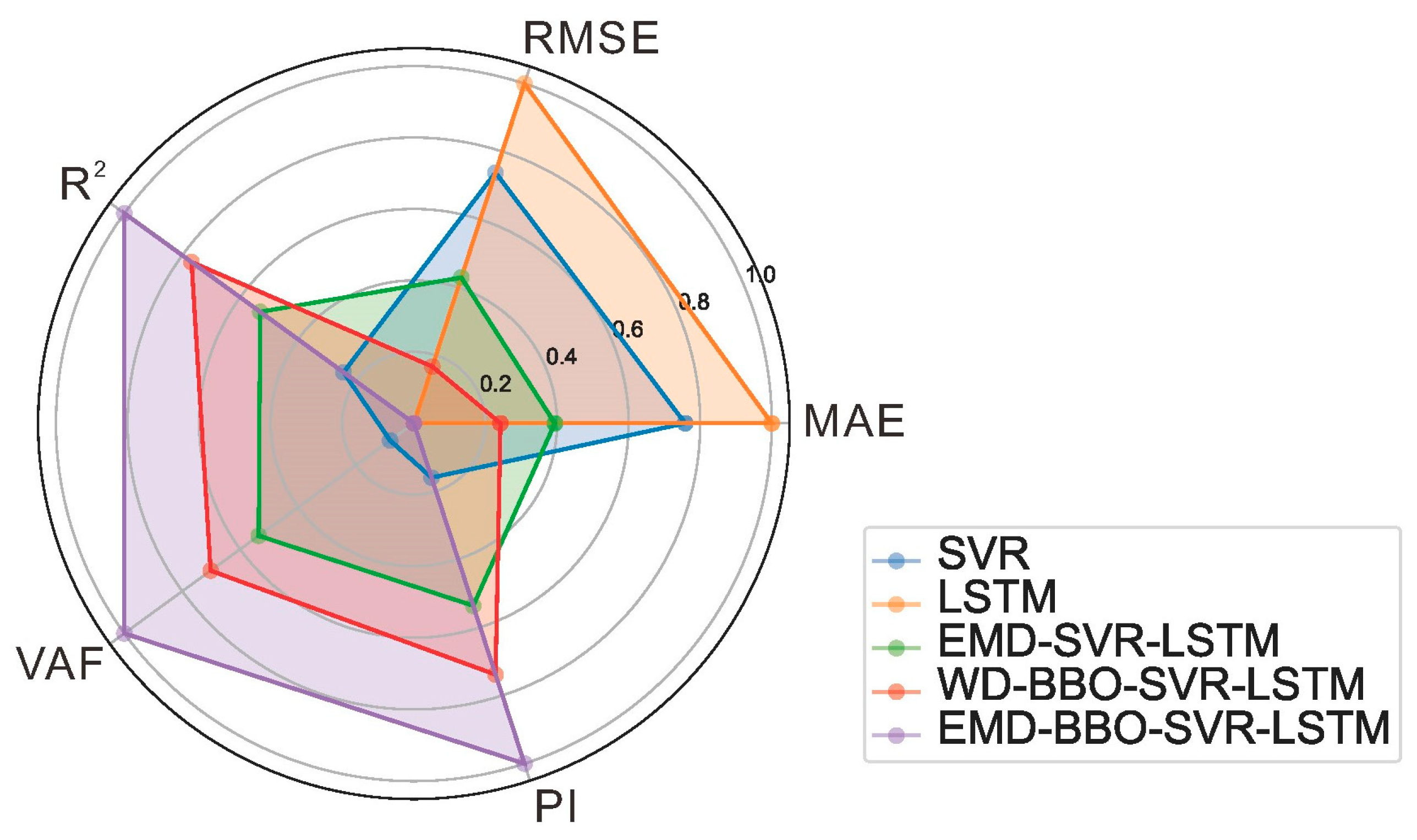
| SVR | 0.075 | 0.105 | 0.794 | 67.69 | 1.366 |
| LSTM | 0.083 | 0.116 | 0.751 | 65.75 | 1.293 |
| EMD-SVR-LSTM | 0.063 | 0.092 | 0.845 | 78.46 | 1.538 |
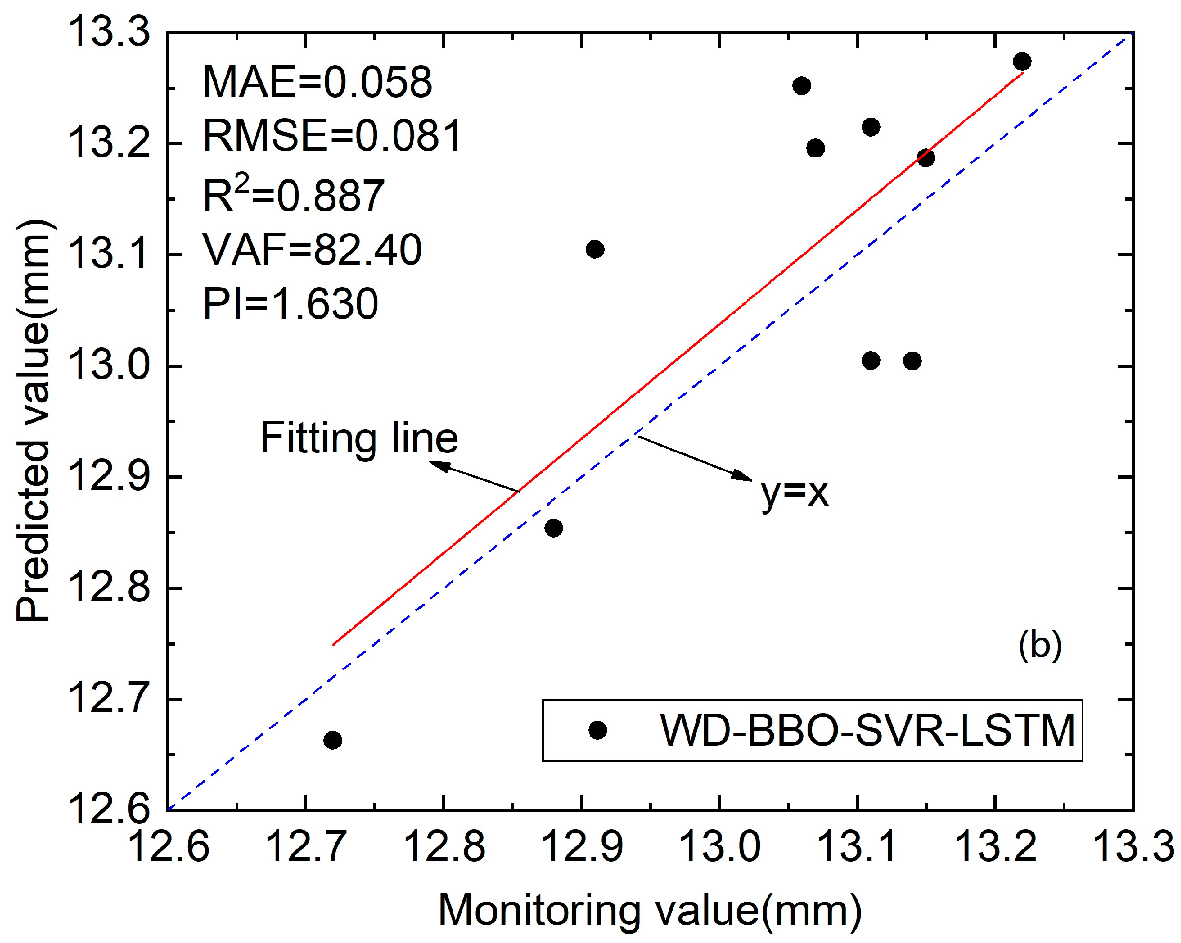
| WD-BBO-SVR-LSTM | 0.058 | 0.081 | 0.887 | 82.40 | 1.630 |
| EMD-BBO-SVR-LSTM | 0.050 | 0.074 | 0.928 | 89.48 | 1.749 |
Disclaimer/Publisher’s Note: The statements, opinions and data contained in all publications are solely those of the individual author(s) and contributor(s) and not of MDPI and/or the editor(s). MDPI and/or the editor(s) disclaim responsibility for any injury to people or property resulting from any ideas, methods, instructions or products referred to in the content. |
© 2023 by the authors. Licensee MDPI, Basel, Switzerland. This article is an open access article distributed under the terms and conditions of the Creative Commons Attribution (CC BY) license (https://creativecommons.org/licenses/by/4.0/).
Share and Cite
Liu, X.; Liu, B. A Hybrid Time Series Model for Predicting the Displacement of High Slope in the Loess Plateau Region. Sustainability 2023, 15, 5423. https://doi.org/10.3390/su15065423
Liu X, Liu B. A Hybrid Time Series Model for Predicting the Displacement of High Slope in the Loess Plateau Region. Sustainability. 2023; 15(6):5423. https://doi.org/10.3390/su15065423
Chicago/Turabian StyleLiu, Xinchang, and Bolong Liu. 2023. "A Hybrid Time Series Model for Predicting the Displacement of High Slope in the Loess Plateau Region" Sustainability 15, no. 6: 5423. https://doi.org/10.3390/su15065423