Abstract
Environmental transformation is a broad and profound economic and social systemic change, which will certainly influence a number of the economic system fields. In particular, does China’s continued low-carbon transition widen the urban–rural income gap while achieving energy conservation and emission reduction targets? This research investigates the effects of low-carbon city pilot (LCCP) programs on urban-rural income gaps and associated mechanisms using a panel of 282 prefecture-level cities from 2007 to 2021. The analysis finds that: (1) LCCP policies exacerbate the urban-rural income disparity in general. In pilot cities, policy implementation widens the urban-rural income difference by roughly 0.5% on average when compared to non-pilot cities. (2) LCCP policies have a direct U-shaped association with employment structure and have a favorable influence on employment structure. (3) The LCCP policies have an inverted U-shaped association with regional innovation capacity, and the LCCP policies have a positive influence on regional innovation capacity. (4) The effects of LCCP policies on urban-rural income disparities vary dramatically between cities based on geography, city size, and resource endowment. The Chinese government should break down market segmentation and encourage urban-rural integration in order to foster technical advancement and scientific and technology innovation, therefore closing the urban-rural income gap and attaining high-quality economic growth in China.
1. Introduction
China is the second largest economy in the world after reform and opening up for over 40 years. On the one hand, China has accomplished high economic growth through a crude economic growth method. On the other hand, a series of challenges such as urban-rural income gap and environmental pollution have been caused. Scholars argue that environmental regulation controls polluting industries to a certain extent and promotes the optimal restructuring of industries but has driven a widening income gap between environmentalists and beneficiaries. Chen Yongwei et al. (2021) [1] points out that with China’s economic development in recent years, income inequality between urban and rural areas has become more and more serious. Others believe that it is an inverted U-shaped relationship between environmental stewardship and income gap, where crossing this barrier will improved income inequality. In China, income inequality is widespread in urban and rural areas, within cities, within villages, and across industries and regions. Zhao Desen et al. (2022) [2] shows that environmental measures can regulate the production behavior of firms. Ultimately, they affect the economic efficiency of firms and the wage income of workers. Recently, China’s State Organizational Structure have been committed to raising people’s income levels, reducing income disparities, and governing the environment. Therefore, in this paper, it is essential to study the relationship between the effects of environmental regulatory policies and income inequality. Currently, China is increasing its environmental protection efforts while income inequality is increasing in society, so this paper attempts to explore whether there is a necessary link between the two.
Environmental pollution is a typical negative externality. Therefore, as the main body governing and protecting the environment, the government has become an important tool. Environmental protection policy is an administrative measure to regulate the production behavior of enterprises and an economic tool to address pollution in the environment and improve quality and efficiency. By studying and learning from the experience of European countries in low carbon economic development, China’s National Development and Reform Commission (NDRC) has launched three batches of Low Carbon City Pilot (LCCP) policies since 2010. A list of cities with LCCP policies in this paper can be found in Appendix A. The three pilot policies were timed for July 2010, November 2012 and January 2017. Although China faced different development tasks during this period, the main objectives of the three batches of pilots are the same. The goal is to control greenhouse gas emissions, explore green low-carbon development models, and demonstrate national low-carbon development. The visionary goal of the LCCP policy is to develop a low-carbon economy, optimize the industrial structure, develop a clean energy structure, build a low-carbon industrial system, and achieve green and sustainable development. If the goal is achieved, then China’s economic growth will be low-carbon and green. China is in a period of economic transformation, and the income distribution pattern will also change.
It has been enthusiastically discussed by the academic community since the LCCP policies was proposed. Most of the relevant literature has been studied about environmental pollution, carbon emission efficiency and innovation. Among them, Du Kerui et al. (2022) [3] LCCP policies can promote the total factor efficiency of carbon emissions in cities. Zhang Hua et al. (2022) [4] found that the pilot cities’ carbon efficiency increased by 2.04% versus the non-pilot cities. In the long term, the effect of LCCP policies will increase gradually. Kuang Haoyu and Xiong Yunjun (2022) [5] concluded that LCCP policies effectively improved green land use efficiency. In addition, Li Muchen et al. (2022) [6] found in a mechanism analysis that industrial structure upgrading and technological innovation promoted the carbon emission reduction effect of LCCP policies. Du Kerui et al. (2022) [3] also found that there are three mediating effect pathways that can enhance the efficiency of carbon emissions. The first is the optimal allocation of resources. The second is the improvement of energy efficiency. The third is the development of green technology innovation. In this paper, we examine whether LCCP policies affect the urban-rural income gap.
The potential contributions of this paper are the following four points. (1) This paper analyzes the income distribution effects of LCCP policies as the available literature mainly studies the environmental effects, economic effects and net policy effects of LCCP policies. (2) This paper selects LCCP policies to represent environmental regulation and specifies the effect of environmental regulation on the urban–rural income gap. (3) This paper investigates the impact mechanism of LCCP policies on the urban–rural income gap in terms of structure and innovation. (4) Different from the previous papers based on regional heterogeneity, this paper also examines the impact of city size heterogeneity and resource endowment heterogeneity. In summary, this paper employs a theoretical approach combined with empirical evidence to conduct a more rigorous analysis of the impact of LCCP policies on the urban-rural income gap, enriching existing research on Porter’s hypothesis from the perspective of LCCP policies and providing some references for future LCCP policy formulation.
The remainder of this research is structured as follows. The second portion provides a literature assessment on LCCP policies and the rural-urban income divide. The third part derives the mathematical model of environmental regulation and income distribution. The mediating theoretical models regarding the structural and innovation effects are also discussed. Further, the three research hypotheses of this study are elicited. The empirical model and data are presented in the fourth section. The fifth part gives the empirical results, including the regression findings of the baseline model, the results of the regional heterogeneity analysis, and the analysis of the mechanism of influence. The sixth part is the conclusion and recommendations with future analysis.
2. Literature Review
2.1. Research Progress of Low-Carbon Cities and LCCP Policies
Domestic and foreign scholars have intensively explored the environmental and economic effects of LCCP policies from the theoretical level. From an environmental point of view, a part of the literature analyzes the impact on the reduction of pollutant emissions. Gehrsitz Markus (2017) [7] found that the German Low Carbon Zone policy has improved local air quality dramatically by decreasing the level of airborne fine particulate matter. Based on a sample of 251 cities in China, Yu Yantuan and Zhang Ning (2021) [8] analyzed the LCCP policies to enhance carbon emission efficiency in the region and the surrounding areas. This indicates that LCCP policies can generate spillover effects to improve carbon emission efficiency. Zeng Shibo et al. (2023) [9] concluded that the LCCP policies can yield spatial spillover effects. And the spillover distance of emission reduction effect of LCCP policies is about 500 meters. From the economic effects aspect, there are also numerous works on the impact of LCCP policies on innovation and economic efficiency. Qiu Shilei et al. (2021) [10] concluded that the LCCP policies promoted green total factor productivity (GTFP) in the pilot cities. Cheng Jinhua et al. (2019) [11] found that the GTFP was about 2.64% higher in the pilot cities than in the other cities. Huang Jingchang et al. (2021) [12] found that the LCCP policy promoted corporate R&D investment, which in turn improved corporate innovation. Wang Taohong et al. (2022) [13] found that the LCCP policies had significant incentives for enterprises to conduct green innovation activities but the effect on enterprises’ green utility innovation behavior was not significant.
2.2. Progress of Research on Factors Influencing Urban–Rural Income Disparity
He Li and Zhang Xiaoling (2022) [14] yielded a Kuznets curve about the relationship between urbanization and income inequality. Among them, the structure of local fiscal expenditures is an effective mediating variable of the income distribution effect of urbanization. Wang Xiang et al. (2019) [15] studied the effects of agricultural production inputs and urbanization on the urban–rural income gap using the system generalized method of moments. The results of the study showed that accelerated urbanization had a significant effect on alleviating the urban–rural income gap. Among them, for provinces with low urbanization, increasing fertilizer application intensity can moderate the disparity, while in provinces with high urbanization, decreasing fertilizer application intensity can reduce the disparity. Using a structural vector autoregressive (SVAR) model, Zhang Quanda and Chen Rongda (2015) [16] f discovered an inverted U-shaped relationship between economic growth and income inequality. Inequality rises in countries during the first stage of financial growth and declines only during the second or even third stage of development. Liu Guanchun et al. (2017) [17] used dynamic generalized moments estimation to confirm a linear inverse U-shaped link between economic growth and income inequality. With the spread of digital technology, it is also critical to investigate the influence of the digital economy on the urban-rural income disparity. Zhao Hongbo et al. (2022) [18] observed that the rise of digital inclusive finance has narrowed the income gap between urban and rural China, with regional differences. Xiong Mingzhao et al. (2022) [19] discovered that developing digital inclusive finance may support regional economic growth and decrease the income gap between urban and rural communities. Furthermore, some academics think that digital economic progress may exacerbate the urban-rural income disparity. Lam Pun-Lee and Shiu Alice (2010) [20] argue that the more economically developed regions develop faster with increased investment in digital infrastructure, while increased investment in digital infrastructure in economically backward regions has no significant impact on local economic development.
2.3. Advances in Research on the Social Impact of Environmental Regulation
The current work on the social repercussions of environmental regulation has mostly examined the effects of environmental regulation on employment. Yamazaki Akio (2017) [21] discovered that the installation of a carbon tax legislation in British Columbia, Canada in 2008 increased overall employment, but the magnitude of the impact differed among industries. Ren Shenggang et al. (2020) [22] analyzed and found that carbon emissions trading promotes employment by expanding the scale of production of enterprises. However, some of the literature suggests that environmental regulation can harm enterprises that use a lot of energy and emit a lot of pollution, resulting in so-called “brown unemployment” in these industries. Based on data from the 1999–2001 Chemical Production Facility Survey, Raff Zach and Earnhart Dietrich (2019) [23] investigated the influence of environmental enforcement on the number of people employed at facilities regulated under the United States Clean Water Act and discovered that the adoption of the law considerably reduced employment. Using firm-level data from 1998–2007, Liu Mengdi et al. (2021) [24] investigated the influence of China’s Air Pollution Prevention and Control Key Cities Delineation Program on corporate environmental pollution and employment and discovered that the strategy decreases employment in manufacturing enterprises. Furthermore, numerous academics have examined the social implications of environmental legislation in terms of income distribution effects. He Xingbang (2019) [25] investigated the impacts of environmental policies based on market incentives and command-and-control on income disparity among urban inhabitants in several regions of China, but the effects of environmental regulations on income inequality were not restricted to urban areas. Specifically, command-and-control environmental laws considerably raise urban residents’ income disparity, but market incentive environmental regulations have no significant influence on urban residents’ income distribution inequality. Bao Tong (2022) [26] investigated the factors influencing the urban-rural income disparity using environmental regulation cost and investment indicators. The study’s findings revealed an inverted U-shaped curve association between both and the urban-rural income disparity. The effect of environmental regulation is to increase and then decrease the income disparity.
In summary, the majority of past research has concentrated on examining the environmental, economic, and employment implications of LCCP regulations. Despite the fact that the number of publications analyzing the social consequences of environmental protection regulations is growing, the following flaws remain. (1) There have been very few studies that analyze the impacts of environmental laws on income distribution patterns, with a particular scarcity of articles assessing the effects of environmental regulations on the establishment of urban-rural equilibrium with income inequality as the major variable. (2) Pollutant emissions, which have historically been used to assess the efficiency of environmental policy implementation, may alter our assessment of policy efficacy. (3) This analysis verifies the LCCP policy’s impact in reducing carbon emissions, increasing green total factor productivity (GTFP), and boosting green innovation. However, it is unclear if the program has had an effect on the urban-rural divide. This is the study’s original starting point and goal. As a result, it is planned to build a time-varying DID model to investigate if and how the LCCP policy impacts the rural-urban income divide.
3. Theoretical Model and Research Hypotheses
The influence of LCCP policies on the urban-rural income gap is examined from a theoretical standpoint in this research, with reference to previous literature. Furthermore, the functions of employment structure and amount of innovation in this are examined.
3.1. A Theoretical Model of Low-Carbon City Pilot Affecting the Urban–Rural Income Gap
Drawing on Barro (1990) [27] to extend the endogenous economic growth model and introduce investment in environmental governance as an important source of public capital, macro production functions are constructed for towns and rural areas. The larger the investment in environmental governance, the greater the intensity of environmental regulation. The production functions for urban and rural areas, respectively, are shown as follows:
where and denote the output level of towns and rural areas, respectively; and denote the technical progress level of towns and rural areas, respectively; denotes the number of labor force in towns and signifies the labor force used in agricultural production, so the total population of the labor force is ; denotes rural land capital; denotes investment in environmental management; and denotes urban physical capital. Assume that rural money is mostly employed for savings and flows to cities via financial markets, and that urban capital is mainly used for investment, urban capital contains two parts: urban residents’ own capital and capital from rural savings , i.e., . Assuming that there are constant returns to scale in the production process, , , and denote the coefficients of output elasticity of the urban labor force, the coefficients of output elasticity of physical capital in towns, the output elasticity of labor in rural areas and the output elasticity of land capital in rural areas, respectively, and , , and are greater than 0 and less than 1. Among them, and denote the coefficients of output elasticity of investment in environmental management in towns and rural areas, respectively.
Given the differences between urban and rural production efficiency and factors of production, and assuming that urban and rural labor markets are perfectly competitive, the price of labor in urban and rural areas depends on the marginal production of labor:
where and denote the regional labor prices in towns and rural areas, respectively, and can be considered as labor wages. Furthermore, assuming that the urban capital market is also perfectly competitive, the urban capital price, i.e., the market interest rate, is determined by the marginal output of capital as follows:
where denotes the marginal output of urban capital. Then, the per capita income of urban and rural residents comes from labor wages and interest income, which is determined by the capital market interest rate for urban residents and the fixed market interest rate for rural residents. Thus, the per capita income of urban and rural residents can be expressed separately as
where and denote the per capita income of urban and rural residents, respectively. On this basis, the Teil index () is introduced to measure the urban–rural income gap, which is calculated as follows:
The is a Thayer index metric used to calculate the urban-rural income disparity. The bigger this score, the greater the income disparity between cities and rural areas. The values of denotes urban and rural areas respectively, denotes the total income of urban or rural area of region , denotes the total income of region , denotes the population size of urban or rural area of region , and denotes the total population of region . Therefore, in this study, the number of population in urban and rural areas are and , respectively, the total urban and rural population is , the overall income of city dwellers is , and remote inhabitants’ total income are denoted as and , respectively. For simplicity of calculation, let and , and then the above equation can be expressed as
To further examine the relationship between the LCCP policies and the Teil index () indicating the urban–rural income gap, the Teil index is used to find the first order derivative of the environmental governance investment .
Since and urban people’ per capita income is often thought to be higher than rural residents’., i.e., , . Thus, we have , . Therefore, the impact of the LCCP policies on the urban–rural income gap depends mainly on , which depends on the relative size of the output elasticity of investment in urban and rural environmental governance. The primary industry is mostly located in rural areas and the secondary and tertiary industries are mostly concentrated in urban areas, and the output value of the primary industry is less affected by environmental management investments than the secondary and tertiary industries. Therefore, it is reasonable to assume that the percentage change in output induced by the established percentage change in investment in environmental management in towns is greater than that of investment in environmental management in rural areas, with other factors of production held constant. Thus, shows that the LCCP policies generate a positive influence on the urban–rural income gap, i.e., the LCCP policies expand the income disparity between urban and rural areas.
Hypothesis 1.
The LCCP policies can promote the urban–rural income gap.
3.2. Mediating Mechanisms of LCCP Policies Affecting Urban–Rural Income Disparity
The LCCP policies cause labor flows from primary industry to the secondary and tertiary industries through promoting the employment structure to high-skilled labor and enhancing the development of regional innovation capacity, which leads to changes in labor demand and supply and relative wage levels, and ultimately affects the urban–rural income gap. The intermediary effects include two main categories.
(1) Structural effects. The structural effect measures the impact of the LCCP policies on the structure of employment. That is, it measures the direct impact of the LCCP policies on the labor market. First, Millimet Daniel L. et al. (2009) [28] point out that environmental regulation raises the production costs of firms, reduces productivity, and also has an impact on the regional employment structure. Second, Porter and Van (1995) [29] indicate that increasing the level of environmental regulation can lead firms to innovate and improve on production technologies that do not meet environmental requirements. Enterprises engage in technological innovation to mitigate environmental costs, which generates innovation compensation effects. Increased technological innovation will optimize the industrial structure and, as a result, the market employment structure. Specifically, the employment structure will see a concentration of employees in the secondary and tertiary industries. This change has increased the labor productivity of the primary industry and increased the income of those working in the primary industry. However, this is just a temporary impact. In the long run, worker productivity in secondary and tertiary sectors will grow dramatically as a result of industrial structure upgrades and technological advancement. As a result, the urban-rural income disparity may narrow in the short run. However, in the long run, it may widen the urban-rural income gap.
Hypothesis 2.
Employment restructuring and upgrading is an intermediary mechanism for LCCP policies to affect the urban–rural income gap.
(2) Innovation effects. According to Li Zheng and Yang Siying (2018) [30], due to the varied invention capacities and innovation effectiveness of the urban and rural industrial sectors, the urban-rural split is the primary cause of the expanding income difference between urban and rural areas. In addition, innovation also causes technology-biased progress, which contributes to the widening of the rural–urban income gap. From a production perspective, the demand elasticity of agriculture products is low, and most of the benefits of technological innovations in agriculture are captured by non-agricultural consumers. The use of new technologies improves the efficiency of agricultural production and increases the market supply of agricultural products. However, the low demand elasticity of agricultural products often leads to an over-supply in the market, triggering a decline in farmers’ income levels. At the same time, consumer residuals in agricultural markets increase instead of the producer residuals due to technological innovations, while producer residuals increase to a lesser extent or are even affected negatively. As a result, it may also happen that the higher the efficiency of agricultural production, the more prominent the contradiction between supply and demand in the market, making the urban–rural income inequality more prominent. Therefore, the increase in regional innovation capacity may widen the urban–rural income gap. The impact of environmental regulation on the urban–rural income gap through regional innovation capacity should be analyzed within two time stages. As agricultural environmental protection policies will increase the production costs of agricultural workers. Consequently, in the short term, agriculture environmental policies will directly reduce the income of agricultural workers and have a minor impact on urban and non-farm workers. Therefore, environmental control measures may push up the urban-rural income gap in the short run. According to the Porter hypothesis, stronger environmental constraints in the long run will promote innovation in social technology. At the same time, the knowledge and technology spillovers from innovation will further reduce the rural-urban income gap. Thus, in the short run environmental regulation may increase the gap, but in the long run effect may reduce the gap.
Hypothesis 3.
The regional innovation level is an intermediary mechanism for LCCP policies to affect the urban–rural income gap.
4. Model Setting and Variable Selection
4.1. Selection of Variables and Data Source
- (1)
- Urban–rural income gap: The Teil index (Teil) is used in this article to measure the urban-rural income disparity. Ji Xuanming et al. (2021) [31] argue that Teil index has more excellent characteristics compared with Gini coefficient. There are three reasons. First, the Teil index can fully take into account the effect of the population base. Second, the Gini coefficient is only sensitive to changes in the middle of the data and does not respond to changes at either end of the data. The Teil index is sensitive to “long tail” data and does not respond to changes in the middle of the data. The gap between rich and poor is reflected at both the high and low income ends of the spectrum. Third, the Teil index can be decomposed into between- and within-groups depending on who is measured. Thus, the Teil index can not only reflect the gap between the high- and low-income ends of the spectrum, but also measure intergroup data well. Therefore, this paper refers to the study of Chen Xu (2019) [32] and uses the Teil index to represent the urban–rural income gap. In the robustness test, this paper uses the urban–rural income ratio (Gapre).
- (2)
- Employment structure effect (LABOR): Referring to the research by Xuan Ye et al. (2019) [33], it is expressed by the ratio of employees in information transmission computer services and software, employees in finance, employees in leasing and business services, and personnel in scientific research, technical services, and geological exploration as a percentage of total employees.
- (3)
- The overall regional innovation level (INNR): Referring to the research by Tang Song et al. (2020) [34], to assess regional innovation capability, the number of regional patent applications was employed. It is expressed by the logarithm of the total number of regional patent applications.
- (4)
- Control variables: Given the complexities of the factors influencing the urban-rural income disparity, this article divides the control variables into macroeconomic growth factors and social development elements. (1) Per capita GDP (PGDP), given as the logarithm of per capita GDP, is a macroeconomic growth factor. (2) Science and technology expenditures (FINT), as measured by the logarithm of science and technology fiscal expenditures. (3) Education expenditure (FI-NE), calculated as the logarithm of education spending in fiscal expenditure. (4) External openness (OPEN), as assessed by the ratio of total actual foreign capital employed to GDP. (5) The degree of financial development (BANK) as assessed by the loan-to-deposit ratio. Population size (POP), calculated as the logarithm of the total population at the end of the year, is one of the social development elements. (2) The urban registered jobless rate (EMP), calculated as the ratio of urban registered unemployed to total population at the end of the year.
4.2. Model Setting Subsection
Considering that the LCCP policy was not proposed at once, it was introduced in three waves. Therefore, the ordinary DID model is not applicable. In this paper, we draw on the model of Beck (2010) [35] to develop a multi-period DID model and include city and time fixed effects in the benchmark regression equation. The specific model setup is shown in Equation (17):
In the above equation, is the explanatory variable urban–rural income gap, is the core explanatory variable of this paper, indicating whether region is a pilot low-carbon city region in year , and region takes the value of 1 if the policy is implemented in year and the rest of the others will be set to 0. is the control variable, is the regional unobserved effect to capture those regional fixed effects that do not change over time, is the time fixed effect to examine the time trend effect, and is the random error term.
Furthermore, the mediating model is used as follows to investigate the influencing mechanism based on Equation (17):
The employment system is represented by LABOR. INNR indicates the total level of regional innovation. Equations (18) and (20) investigate whether LCCP regulations have a substantial influence on the regional employment structure and overall level of innovation. Equations (19) and (21) are utilized to investigate the intermediate effect of LCCP policies on the urban-rural income gap, with the goal of determining whether the employment structure and overall regional innovation level may be employed as a mediating variable. In this model, the main concern is the coefficients , and . denotes the net effect of the mediating variable, and and measure the effect of the mediating variable on the urban–rural income gap. All additional variables can be understood similarly to Equation (17).
4.3. Data Introduction
The sample for this research is data from 282 Chinese prefecture-level cities. The sample years of this paper are 2007–2021. The data for the variables are obtained from the China City Statistical Yearbook (https://data.cnki.net/yearBook, accessed on 1 January 2022.) and Statistical Bulletin of National Economic and Social Development (http://www.stats.gov.cn/tjsj/tjgb/ndtjgb, accessed on 1 January 2022.) in previous years, and some missing data have been filled in by the interpolation method. This paper uses Stata 17.0 for data processing and analysis. Table 1 contains the descriptive statistics for the data.

Table 1.
Definition and the variables’ descriptive statistics.
5. Methodology and Materials
5.1. Baseline Model Regression Result
Table 2 shows the estimated effects of low-carbon pilot cities on the urban-rural income divide. Column (1) demonstrates that the urban-rural income gap narrows by 0.0265 in low-carbon pilot cities compared to non-low-carbon pilot cities, and that this difference is significant at the 1% level. However, because this model does not account for macroeconomic and social issues, the results may be insufficiently robust. Columns (2) to (4) include both macroeconomic level and social development level control variables, and the regression coefficient is found to be 0.008 when time fixed effects and city fixed effects are not taken into account; when time fixed effects are taken into account, the regression coefficient of the urban-rural income gap for implementing low-carbon pilot cities decreases by 0.002, but does not pass the 10% significance level test. In column (4), the urban–rural income gap increases by 0.005 in low-carbon pilot cities compared with non-low-carbon pilot cities and is significant at the 10% level of significance. The results are more robust because column (4) considers both time fixed effects and area fixed effects, which alleviates the endogeneity problem of omitted variable bias to a certain extent. Therefore, through the baseline regression, it is tentatively concluded that the LCCP policies significantly increase the income gap in the pilot cities. The empirical findings verify the accuracy of Hypothesis 1 “The LCCP policies can increase the urban–rural income gap”.
Table 2.
The impact of low-carbon city pilot policies on urban–rural income disparity.
Further examination of the regression findings in Column (4) of Table 2 reveals that (1) the GDP per capita coefficient is strongly negative, showing that economic expansion is favorable to closing the urban-rural income gap. (2) The population size coefficient on the urban-rural income difference is considerably positive, indicating that increasing population size is not favorable to closing the urban-rural income disparity. (3) The coefficient of the effect of the degree of openness to the outside world is negative, indicating that increasing openness to the outside world will shrink the income difference between urban and rural areas. (4) The coefficient of fiscal expenditure on science and technology is positive but insignificant, indicating that additional investment in science and technology, as well as improvements in the accuracy of science and technology services, are required to close the income gap; the coefficient of education expenditure is significantly negative, indicating that the “education tendency” of fiscal expenditure will close the income gap between urban and rural areas. (5) The coefficient of financial development level is positive but insignificant because financial resources are highly concentrated and unevenly distributed in urban areas, and their scarcity and inefficiency in rural areas impede the growth of rural household income, widening the urban-rural income gap. As a result, it is critical to ensure that financial resources develop in both urban and rural regions in a balanced manner. (6) The effect of the urban registered unemployment rate on the urban-rural income difference is positive but not statistically significant, showing that finding work can help to close the urban-rural income gap to some extent.
5.2. Parallel Trend Test
The parallel trend test is a test that must be performed for the double-difference model. Because it is difficult to know whether the change in Y is due to policy implementation, the parallel trend test should show that there is no significant difference between the control and experimental groups prior to policy implementation. The baseline regression in this paper verifies that the LCCP policy widens the urban-rural income gap. As a result, in order to rule out baseline regression instability owing to a violation of the “parallel trend” assumption. In this paper, we use event analysis to examine the effect of the policy over time and to test the assumption of parallel trends.
indicates the implementation of LCCP policies in the city. If city starts LCCP policies in year , then = 1, otherwise = 0. As can be seen from Vertical line in Figure 1 denotes the year when the first low-carbon municipal pilot strategy was enacted. The year is 2010 in this document. All of the outcomes prior to 2010 reveal no cause to reject the original premise. Then, before the year of policy implementation, it may be assumed that there is no substantial variation in the urban-rural income gap between the experimental and control groups. As a result, the parallel trend test is successful.
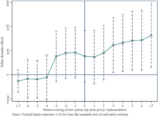
Figure 1.
Parallel trend chart.
5.3. Robustness Check
- (1)
- Replacing the explanatory variable metrics.
The urban-rural income ratio is used in this study to replace the Teil index in measuring the urban-rural income gap, with the goal of testing the robustness of the baseline regression results. Table 3 column (1) displays the regression findings, where the coefficient of LCCP is significantly positive at 0.0531. This suggests that LCCP policy contributes to the widening of the urban-rural income disparity, as assessed by the urban-rural income ratio. This results in a strong baseline regression result.
Table 3.
A set of robustness tests.
- (2)
- Excluding other policy effects.
Due to the long span of the selected years, other contemporaneous policies may affect the urban–rural income gap in the pilot cities. This paper collects and collates one policy that overlaps with the study sample interval based on the Notice of the NDRC on Promoting the Pilot Work of National Innovative Cities (Development and Reform High Technology (2010) No. 30). To exclude the interference of the above policy, a time-varying DID dummy variable for the relevant policy is further included in the regression, where Innov * post is whether the national innovative city pilot work is implemented. The results are presented in Column (2) of Table 3, where it can be seen that the estimated coefficient of the LCCP policies remains significantly positive.
- (3)
- Propensity Score Matching Differences-in-Differences model (PSM-DID).
In this paper, PSM-DID is used to mitigate the interference of the baseline regression model results due to sample selection bias and other potential endogeneity issues. According to Guo Xinglei et al. (2023) [36] control variables are selected as matching variables. In this paper, the caliper nearest neighbor matching method was used. The balance test revealed a substantial reduction in standardized bias for all variables, which indicates good matching. t-test results showed no reason to reject the original hypothesis, which indicates no significant difference between the experimental and control groups. The results of these two tests show that the PSM-DID method conforms to the requirements of a randomized trial, effectively reducing systematic differences between the two sample groups and alleviating the endogeneity problem caused by sample self-selection. The regression results are presented in column (1) of Table 4, which shows that the dummy variable LCCP has a significant coefficient of 0.0046, so the baseline regression results are robust.
Table 4.
A set of endogeneity tests.
- (4)
- Instrumental Variable Analysis
By establishing instrumental variables, this research solves the endogeneity problem created by the non-random selection of policy pilot cities. Referring to Shi Dan and Li Shaolin (2020) [37], the natural logarithm of the annual average of the city’s air circulation coefficient (lnVC) is chosen as the instrumental variable for the LCCP. There is an inverse relationship between the air circulation coefficient of a city and the monitored pollution concentration. When the value of total pollutant emissions is controlled, the smaller the air circulation coefficient of a city, the stronger the government is likely to strengthen environmental regulation. Through the above analysis, the correlation hypothesis is satisfied between the air circulation coefficient and the LCCP policies. Since the air circulation coefficient is not affected by the urban-rural income gap, it better satisfies the exogeneity hypothesis. The results are shown in column (2) of Table 4, where the coefficients of the air circulation coefficient and the time variable interaction term lnVC * post are significantly positive, and the estimated coefficient of the LCCP policies in column (3) is significantly positive. 2SLS approach is consistent with the results of the baseline regression, indicating that the baseline regression results are robust.
5.4. Heterogeneity Analysis
- (1)
- Locational heterogeneity. There are large regional differences in China, with the eastern region developing rapidly, having natural ports, better levels of technological innovation, foreign direct investment, and infrastructure than the central and western regions, which also causes a large number of laborers from the central and western regions to move to the eastern region. As a result, following on the work of Li Yanling et al. (2022) [38], this study divides the sample into eastern, central, and western sectors in order to evaluate the various effects of building low-carbon cities in different locations on the urban-rural income gap. As a consequence, based on the regression findings provided in Table 5, the LCCP policies have a considerable expanding influence on the urban-rural income difference in the eastern area. The urban-rural income disparity in eastern low-carbon cities is 0.0077 units more than in non-pilot cities, and the coefficient is significant at the 1% level. However, the coefficients of LCCP policies are not significant in either the central or western regions. It is strongly suggested that the phenomenon of widening urban–rural income gaps due to LCCP policies mainly arises in the eastern region, which also proves the existence of locational heterogeneity. In addition, the coefficient of the LCCP variable is 0.005 for the full sample (column 4 of Table 2) and 0.0077 for the eastern region. The comparison results indicate that the LCCP policies have a greater impact on widening the urban–rural income gap in the eastern region.
Table 5. Heterogeneous analysis at regional, city size and resource endowment levels.
- (2)
- City-scale heterogeneity. LCCP policies’ impact on the urban-rural income gap probably varies by city size. As shown in Table 5, the effect of LCCP policies implementation on urban–rural income gap is manifested in mega-cities, but not yet significant in other cities. It is possible that the development of mega-cities basically relies on the service industry, and the LCCP policies enable the industrial structure upgrading effect to be more apparent, which further widens the urban–rural income gap.
- (3)
- Resource endowment heterogeneity. Wen Shiyan et al. (2022) [39] point out that the resource endowments on which urban development depend are the basis for influencing urban innovation. In this regard, this paper examines the heterogeneous impact of LCCP policies on urban–rural income disparity from the perspective of urban resource endowment differences. Based on the Notice of the State Council on the Issuance of the National Sustainable Development Plan for Resource-based Cities (2013–2020) (Guo Fa (2013) No. 45), this paper divides the 282 sample cities into 113 resource cities and 169 non-resource cities. Observing columns (6) and (7) of Table 5, it can be observed that the LCCP policies widen the urban–rural income gap in non-resource cities and have a negative effect on resource cities, i.e., they can reduce the urban–rural income gap, but this effect does not pass the 10% significance level test, a finding similar to the scholar Gao Da et al. (2022) [40]. Compared with resource-endowed cities, the development of non-resource-based cities relies more on the optimization of industrial structure, and under the influence of LCCP policies, more attention is paid to the scale expansion of tertiary industries as well as the innovative development of secondary industries, thus significantly widening the urban–rural income gap.
5.5. Mediating Effect Analysis
Through the previous analysis, we find that there is an effect of LCCP policies on income disparity. However, if we want to analyze clearly how to guide the LCCP policies to alleviate the income gap between rural and urban areas, we need to know clearly the possible impact paths. Therefore, in this section, we focus on analyzing the impact mechanism. Supported by the prior theoretical model, we find that employment structure and innovation are potential impact paths. Therefore, we analyze the impact mechanism from two perspectives: the structure effect and the innovation effect.
- (1)
- Structural effect
Column (1) of Table 6 indicates that the LLCP policies have a mediating effect of employment structure in shaping the development of urban and rural income. The coefficient of the dummy variable LCCP, which means LLCP policies, is 0.0038, which cleared the 90% significance level test. This shows that the LLCP policies can promote the restructuring of employment toward advanced levels, which is consistent with the previous theoretical analysis. The mediation effect can be further judged from column (2) where it can be seen that with the inclusion of the LABOR variable and the quadratic term, the coefficient of the dummy variable LCCP, which represents the LLCP policies, is significant at 0.0043, the coefficient of the LABOR variable is −0.0874, and the coefficient of the quadratic term of the LABOR variable is significant 0.6829. The insignificant coefficient of employment structure indicates that the positive effect of employment structure on narrowing the urban-rural income gap in the low-carbon pilot cities has not yet taken effect. the coefficient of the quadratic term of the LABOR variable is significantly positive, indicating a U-shaped curve between advanced employment structure and the urban-rural income gap. The index of advanced employment structure at the turning point is calculated to be 0.064, indicating that the urban-rural income gap decreases due to employment restructuring at the beginning of the transition to an advanced employment structure, but gradually widens after the peak of employment restructuring. This finding is consistent with the previous theoretical analysis. Therefore, Hypothesis 2, “employment restructuring and upgrading is the mediating mechanism of the effect of LCCP policies on the urban–rural income gap”, is verified.
Table 6.
Mechanism analysis of structural effects.
- (2)
- Innovation effect
Column (1) of Table 7 shows the outcomes of the LCCP policy’s influence on the number of patents awarded. The LCCP coefficient is highly positive, which is consistent with the preceding theoretical study. This indicates that the LCCP policy promotes the level of innovation development in the pilot regions. Similarly, the level of innovation has a mediating effect in terms of the LCCP policy affecting the urban-rural income gap. Column (2) adds the INNR variable and the quadratic term. The coefficient of the dummy variable LCCP is 0.0025, the coefficient of the INNR variable is 0.1082, and the coefficient of the quadratic term of the INNR variable is −0.0478, all of which are highly significant. Since the quadratic coefficient of INNR variable is significantly negative, there is an inverted U-shaped relationship between regional innovation level and the urban–rural income gap. According to the calculation results, the inflection point of the inverted U-shaped curve is 1.1317, which means that when the patent grant is less than 1.1317, the LCCP policies widen the urban–rural income gap through patent grants, and conversely, when the patent grants exceed 1.1317, the LCCP policies narrow the urban–rural income gap through patent grants. This finding is consistent with the previous theoretical analysis and the results of scholar Ma Guoqun (2022) [41]. Therefore, Hypothesis 3, “the regional innovation level is a mediating mechanism for the effects of LCCP policies on the urban–rural income gap,” is proven.
Table 7.
Mechanism analysis of innovation effect.
6. Conclusions and Policy Recommendations
6.1. Conclusions
This study makes the following findings based on panel data from 282 Chinese cities from 2007 to 2021:
First, the LCCP policy had a considerable influence on the urban-rural income disparity in the trial towns, lending credence to the first hypothesis that LCCP policies might encourage an increase in the urban-rural income gap. When compared to non-pilot cities, the urban-rural income gap grew by about 0.5% on average in the trial cities. This finding holds after parallel trend tests and robustness tests, such as sample data screening, inclusion of benchmark variables, exclusion of other policy interferences and propensity score matching. Second, the impacts of LCCP policies vary according to area, city size, and resource endowment. In eastern areas, megacities, and non-resource-endowed regions, LCCP measures successfully widen the urban-rural income disparity. On the other side, the impact on the central and western areas, small and medium-sized towns, and resource endowment regions is uncertain. Third, in the short term, the LCCP policies reduce the urban–rural income gap by optimizing the employment structure; however, in the long term, the LCCP policies widen the urban–rural income gap by challenging the employment structure. Hypothesis 2, “Employment structure is the mediating mechanism of the effect of LCCP policies on the urban–rural income gap”, is verified. In contrast to the mediating effect played by employment structure, the mediating effect played by regional innovation capacity has an inverted U-shape. In the short term, LCCP policies widen the urban–rural income gap by enhancing regional innovation capacity. In the long run, LCCP policies reduces the urban–rural income gap through regional innovation capacity. Hypothesis 3, “Regional innovation capacity is a mediating mechanism for the effects of LCCP policies on the urban–rural income gap”, is verified.
The reasons for this result are analyzed as follows:
First, the process of achieving low-carbon development intensifies the dual structure between urban and rural areas. LCCP policies mainly restrict carbon emissions, which leads to rises in the environmental management costs of enterprises and declines in enterprise output. This has an impact on the labor market, producing structural unemployment and contributing to the economic disparity between urban and rural areas. Furthermore, in order to accomplish development, energy conservation, and emission reduction, businesses will engage in technical innovation and improve their market competitiveness. This phenomenon brings new employment opportunities on the one hand, and eliminates some backward jobs on the other, causing structural unemployment. Second, the labor productivity of each industry in urban and rural areas is different under the dual economic structure of urban and rural areas in China. The LCCP policies transform the labor force from low-skilled labor to medium and high-skilled labor and move it from the primary to the secondary and tertiary industries through two pathways, ultimately causing changes in labor supply and demand and wage rates. The first pathway is the structural effect of promoting a change in the employment structure toward a higher-skilled labor force. The second pathway is the innovation effect of promoting the development of overall regional innovation capacity and green innovation capacity. This in turn affects the urban–rural income gap. Third, the low-carbon city pilot primarily encourages high-quality growth in major cities, which can better execute LCCP regulations than small and medium-sized cities due to well-developed infrastructure and tight policy implementation processes. As a result, the effect of the low-carbon city pilot strategy on major cities is more visible. The eastern area is more vulnerable to strong environmental regulation measures since it is more economically developed and has a more robust industrial foundation. However, the central and western regions have weaker industrial development compared to the eastern regions. Even if the central and western regions increase investment in environmental management, the effect may still be insignificant.
6.2. Policy Recommendations
Based our findings, this paper proposes the following policy recommendations.
First, the supporting policies related to environmental regulation should be improved. When developing environmental regulations, it is critical to examine not just the influence on the natural environment, but also the impact on society and people’s livelihoods., especially the affordability of environmental policies for individuals and enterprises, and whether social welfare and people’s happiness will be reduced due to the intensity of policies. Therefore, the intensity of policies should be set at a reasonable level. If necessary, some supporting policies can be introduced, such as subsidies to polluting enterprises, assistance to set up pollution control equipment, etc. In terms of policy tools, priority should be given to market-based tools, giving enterprises some freedom of choice and implementing continuous incentives for them.
Second, China should actively coordinate the balanced development of employment structure and industrial structure. Currently, China is in the phenomenon of rapid upgrading of industrial structure but lagging employment structure. At this stage, China should deepen the reform of agricultural modernization, actively develop modernized agriculture, and coordinate the relationship between technology- and capital-intensive manufacturing and modernized agriculture. In due course, it should absorb surplus rural labor, build a reasonable and advanced employment structure, and promote the development of the same direction of industrial and employment structures. While vigorously developing agricultural modernization, introduce secondary and tertiary industries into rural areas in a moderate and reasonable manner to expand and enhance farmers’ income sources and alleviate the income gap between urban and rural areas. The government should support rural enterprises to develop processing, logistics, transportation and other related industries in rural areas, so as to improve the added value of agricultural products, promote the circulation of agricultural products, and gradually realize the transformation from labor-intensive to capital-intensive industries.
Third, the government’s functions in governing the environment and narrowing the gap between the rich and the poor should be reflected more prominently. The government can alleviate urban-rural income inequality through measures such as increasing expenditures on science and technology, education and social security. In addition, government regulatory measures such as eliminating the household registration system are also beneficial in alleviating the pressure of urban-rural inequality. Therefore, it is important to moderately increase urbanization level and government fiscal expenditures to ensure stable economic operation, promote the improvement of local government functions, ensure the implementation of fiscal expenditures, and pay attention to the reform and upgrading of rural industries in order to narrow the urban-rural income gap.
6.3. Deficiencies and Prospects
The influence of LCCP policies on the urban-rural income gap has been analyzed in depth in this study. However, we still believe that the limitations of the study should be considered when analyzing related issues. This study analyzes the income distribution effects of LCCP policies through a double difference model. Through extensive reading of the literature, it is found that LCCP policies also have some effects in space. Therefore, it is recommended to use spatial econometric analysis combined with double difference models in further analysis to analyze the effect of LCCP policies on urban-rural income disparity.
Author Contributions
Conceptualization, Z.Z.; methodology, Z.Z.; software, T.C.; validation, Z.Z. and T.C.; formal analysis, Z.Z. and T.C.; investigation, Z.Z.; resources, T.C.; data curation, T.C.; writing—original draft preparation, Z.Z. and T.C.; writing review and editing, T.C.; visualization, Z.Z.; supervision, Z.Z.; project administration, Z.Z.; funding acquisition, Z.Z. All authors have read and agreed to the published version of the manuscript.
Funding
This research was funded by National Social Science Foundation of China. Fund grant number: 21BJL107.
Institutional Review Board Statement
Not applicable.
Informed Consent Statement
Not applicable.
Data Availability Statement
Publicly available datasets were analyzed in this study. These data can be found here: China Statistical Yearbook (2008–2022), China Urban Statistical Yearbook (2008–2022), and China Economic Network Statistical.
Conflicts of Interest
The authors declare no conflict of interest.
Appendix A
The first batch of pilots was launched on 19 July 2010 and included Hubei Province, Yunnan Province, Guangdong Province, Shaanxi Province, Liaoning Province and Chongqing City, Xiamen City, Nanchang City, Baoding City, Tianjin City, Shenzhen City, Hangzhou City, and Guiyang City. The second batch of pilots was determined on 26 November 2012 and included Beijing City, Shanghai City, Hainan Province and Qinhuangdao City, Hulunbeier City, Daxinganling Region, Huaian City, Ningbo, Nanping, Ganzhou, Jiyuan, Guangzhou, Zunyi, Kunming, Yan’an, Shijiazhuang, Jincheng, Jilin, Suzhou, Zhenjiang, Wenzhou, Chizhou, Jingdezhen, Qingdao, Wuhan, Guilin, Guangyuan, Jinchang, and Urumqi. The third batch of pilots began on 7 January 2017 in Wuhai, Dalian, Sunk County, Changzhou Jinhua, Hefei, Huangshan, Xuancheng, Liuan, Gongqingcheng, Fuzhou, Jinan, Yantai, Changsha, Chenzhou, Zhongshan, Liuzhou, Chengdu, Yuxi, Ankang, Dunhuang, Yinchuan, Wuzhong, Yining, Hotan, Alar, Division I, Shenyang, Chaoyang, Nanjing, Jiaxing, Quzhou, Huaibei, Sanming, Ji’an, Weifang Changyang Tujia Autonomous County, Zhuzhou City, Xiangtan City, Sanya City, Qiongzhong Li Miao Autonomous County, Smao District, Pu’er City, Lhasa City, Lanzhou City, Xining City, and Changji City.
References
- Chen, Y.W.; Fu, D.H.; Ye, X.Y. Income comparison and happiness: The role of fair income distribution. Aust. Econ. Pap. 2021, 60, 41–63. [Google Scholar] [CrossRef]
- Zhao, D.S.; Dou, Y.; Tong, L. Effect of fiscal decentralization and dual environmental regulation on green poverty reduction: The case of China. Resour. Policy 2022, 79, 102990. [Google Scholar] [CrossRef]
- Du, K.R.; Cheng, Y.Y.; Yao, X. Environmental regulation, green technology innovation, and industrial structure upgrading: The road to the green transformation of Chinese cities. Energy Econ. 2021, 98, 105247. [Google Scholar] [CrossRef]
- Zhang, H.; Feng, C.; Zhou, X.X. Going carbon-neutral in China: Does the low-carbon city pilot policy improve carbon emission efficiency. Sustain. Prod. Consum. 2022, 33, 312–329. [Google Scholar] [CrossRef]
- Kuang, H.Y.; Xiong, Y.J. Could environmental regulations improve the quality of export products? Evidence from China’s implementation of pollutant discharge fee. Environ. Sci. Pollut. Res. 2022, 29, 81726–81739. [Google Scholar] [CrossRef]
- Li, M.C.; Feng, S.X.; Xie, X. Spatial effect of digital financial inclusion on the urban-rural income gap in China-analysis based on path dependence. Econ. Res.-Ekon. Istraz. 2023, 36, 2999–3020. [Google Scholar] [CrossRef]
- Gehrsitz, M. The effect of low emission zones on air pollution and infant health. J. Environ. Econ. Manag. 2017, 83, 121–144. [Google Scholar] [CrossRef]
- Yu, Y.; Zhang, N. Low-carbon city pilot and carbon emission efficiency: Quasi-experimental evidence from China. Energy Econ. 2021, 96, 105125. [Google Scholar] [CrossRef]
- Zeng, S.; Jin, G.; Tan, K.; Liu, X. Can low-carbon city construction reduce carbon intensity? Empirical evidence from low-carbon city pilot policy in China. J. Environ. Manag. 2023, 332, 117363. [Google Scholar] [CrossRef]
- Qiu, S.; Wang, Z.; Liu, S. The policy outcomes of low-carbon city construction on urban green development: Evidence from a quasi-natural experiment conducted in China. Sustain. Cities Soc. 2021, 66, 102699. [Google Scholar] [CrossRef]
- Cheng, J.; Yi, J.; Dai, S.; Xiong, Y. Can low-carbon city construction facilitate green growth? Evidence from China’s pilot low-carbon city initiative. J. Clean. Prod. 2019, 231, 1158–1170. [Google Scholar] [CrossRef]
- Huang, J.; Zhao, J.; Cao, J. Environmental regulation and corporate R&D investment-evidence from a quasi-natural experiment. Int. Rev. Econ. Financ. 2021, 72, 154–174. [Google Scholar] [CrossRef]
- Wang, T.; Song, Z.; Zhou, J.; Sun, H.; Liu, F. Low-Carbon Transition and Green Innovation: Evidence from Pilot Cities in China. Sustainability 2022, 14, 7264. [Google Scholar] [CrossRef]
- He, L.; Zhang, X. The distribution effect of urbanization: Theoretical deduction and evidence from China. Habitat Int. 2022, 123, 102544. [Google Scholar] [CrossRef]
- Wang, X.; Shao, S.; Li, L. Agricultural inputs, urbanization, and urban-rural income disparity: Evidence from China. China Econ. Rev. 2019, 55, 67–84. [Google Scholar] [CrossRef]
- Quanda Zhang, R.C. Financial Development and Income Inequality in China: An Application of SVAR Approach. Procedia Comput. Sci. 2015, 55, 774–781. [Google Scholar] [CrossRef]
- Liu, G.; Liu, Y.; Zhang, C. Financial Development, Financial Structure and Income Inequality in China. World Econ. 2017, 40, 1890–1917. [Google Scholar] [CrossRef]
- Zhao, H.; Zheng, X.; Yang, L. Does Digital Inclusive Finance Narrow the Urban-Rural Income Gap through Primary Distribution and Redistribution? Sustainability 2022, 14, 2120. [Google Scholar] [CrossRef]
- Xiong, M.; Li, W.; Teo, B.S.X.; Othman, J. Can China’s Digital Inclusive Finance Alleviate Rural Poverty? An Empirical Analysis from the Perspective of Regional Economic Development and an Income Gap. Sustainability 2022, 14, 6984. [Google Scholar] [CrossRef]
- Lam, P.-L.; Shiu, A. Economic growth, telecommunications development and productivity growth of the telecommunications sector: Evidence around the world. Telecommun. Policy 2010, 34, 185–199. [Google Scholar] [CrossRef]
- Yamazaki, A. Jobs and climate policy: Evidence from British Columbia’s revenue-neutral carbon tax. J. Environ. Econ. Manag. 2017, 83, 197–216. [Google Scholar] [CrossRef]
- Ren, S.; Liu, D.; Li, B.; Wang, Y.; Chen, X. Does emissions trading affect labor demand? Evidence from the mining and manufacturing industries in China. J. Environ. Manag. 2020, 254, 109789. [Google Scholar] [CrossRef]
- Raff, Z.; Earnhart, D. The effects of Clean Water Act enforcement on environmental employment. Resour. Energy Econ. 2019, 57, 1–17. [Google Scholar] [CrossRef]
- Liu, M.; Tan, R.; Zhang, B. The costs of “blue sky”: Environmental regulation, technology upgrading, and labor demand in China. J. Dev. Econ. 2021, 150, 102610. [Google Scholar] [CrossRef]
- He, X. Investigating Environmental Regulation and Income Inequality of Urban Residents--The Perspective of Idiosyncratic Regulatory Tools. Collect. Essays Financ. Econ. 2019, 247, 104–112. [Google Scholar] [CrossRef]
- Tong, B. Has Environmental Regulation Widened or Narrowed the Urban-rural Income Gap? Based on the Dual Perspectives of Economic Efficiency and Economic Structure. J. Yunnan Univ. Financ. Econ. 2022, 38, 1–20. [Google Scholar] [CrossRef]
- Barro, R.J. Government Spending in a Simple Model of Endogeneous Growth. J. Political Econ. 1990, 98, 103–125. [Google Scholar] [CrossRef]
- Millimet, D.L.; Roy, S.; Sengupta, A. Environmental Regulations and Economic Activity: Influence on Market Structure. Annu. Rev. Resour. Econ. 2009, 1, 99–117. [Google Scholar] [CrossRef]
- Porter, M.; Van der Linde, C. Green and competitive: Ending the stalemate. Harv. Bus. Rev. 1995, 73, 120–134. [Google Scholar]
- Li, Z.; Yang, S. The urban-rural dual income structure effect of science and technology innovation and its transmission mechanism. Inq. Into Econ. Issues 2018, 426, 23–29. [Google Scholar] [CrossRef]
- Ji, X.M.; Wang, K.; Xu, H.; Li, M.C. Has Digital Financial Inclusion Narrowed the Urban-Rural Income Gap: The Role of Entrepreneurship in China. Sustainability 2021, 13, 8292. [Google Scholar] [CrossRef]
- Xu, C. Urban sprawl, geographical agglomeration and urban-rural income gap. Ind. Econ. Res. 2019, 100, 40–51. [Google Scholar] [CrossRef]
- Xuan, Y.; Lu, J.; Yu, Y. The Impact of High-speed Rail Opening on the Spatial Agglomeration of High-end Service Industry. Financ. Trade Econ. 2019, 40, 117–131. [Google Scholar] [CrossRef]
- Tang, S.; Wu, X.; Zhu, J. Digital Finance and Enterprise Technology Innovation:Structural Feature, Mechanism Identification and Effect Difference under Financial Supervision. J. Manag. World 2020, 36, 52–66. [Google Scholar]
- Beck, T.; Levine, R.; Levkov, A. Big Bad Banks? The Winners and Losers from Bank Deregulation in the United States. J. Financ. 2010, 65, 1637–1667. [Google Scholar] [CrossRef]
- Guo, X.L.; Qian, Z.; Yin, Z.L.; Li, Z.H.; Shao, C.Z. Research on the impact of China’s urban rail transit on economic growth: Based on PSM-DID model. Front. Environ. Sci. 2023, 11, 1082567. [Google Scholar] [CrossRef]
- Shaolin, S.D.L. Emissions Trading System and Energy Use Efficiency—Measurements and Empirical Evidence for Cities at and above the Prefecture Level. China Ind. Econ. 2020, 390, 5–23. [Google Scholar] [CrossRef]
- Li, Y.; Wang, M.; Liao, G.; Wang, J. Spatial Spillover Effect and Threshold Effect of Digital Financial Inclusion on Farmers’ Income Growth-Based on Provincial Data of China. Sustainability 2022, 14, 1838. [Google Scholar] [CrossRef]
- Wen, S.Y.; Jia, Z.J.; Chen, X.Q. Can low-carbon city pilot policies significantly improve carbon emission efficiency? Empirical evidence from China. J. Clean. Prod. 2022, 346, 131131. [Google Scholar] [CrossRef]
- Gao, D.; Li, Y.; Li, G. Boosting the green total factor energy efficiency in urban China: Does low-carbon city policy matter? Environ. Sci. Pollut. Res. 2022, 29, 56341–56356. [Google Scholar] [CrossRef]
- Ma, G.Q.; Lv, D.Y.; Luo, Y.X.; Jiang, T.B. Environmental Regulation, Urban-Rural Income Gap and Agricultural Green Total Factor Productivity. Sustainability 2022, 14, 8995. [Google Scholar] [CrossRef]

Disclaimer/Publisher’s Note: The statements, opinions and data contained in all publications are solely those of the individual author(s) and contributor(s) and not of MDPI and/or the editor(s). MDPI and/or the editor(s) disclaim responsibility for any injury to people or property resulting from any ideas, methods, instructions or products referred to in the content. |
© 2023 by the authors. Licensee MDPI, Basel, Switzerland. This article is an open access article distributed under the terms and conditions of the Creative Commons Attribution (CC BY) license (https://creativecommons.org/licenses/by/4.0/).