Abstract
With the acceleration of urbanization, problems such as urban ecological environment quality have become increasingly prominent. How to scientifically analyze and evaluate the spatial pattern of urban ecological environment changes and influential variables is a prerequisite for achieving green development and ecological priority new in urban planning. Our study was conducted on Pingtan Island, located in Fujian Province, China. First, we selected Landsat 8 OLI images in 2013, 2017, and 2021. Second, we extracted the remote sensing ecological index (RSEI) from these images and created RSEI maps to assess the spatial-temporal variations and spatial autocorrelation of the ecological environment condition in Pingtan Island. Third, the proportion of land-use types, road, and population density were selected as independent variable factors, RSEI as the dependent variable, least squares regression (OLS), geographically weighted regression (GWR), and multi-scale geographically weighted regression (MGWR) were used to establish global and local regression models. According to the regression coefficients of the model and its spatial distribution, the spatial heterogeneity between the ecological environment and the influencing factors was assessed. The results indicated that: (1) the mean value of the RSEI increased from 0.422 to 0.504 during 2013–2021, indicating that the overall ecological environment improved. (2) Based on the global Moran’s I value, the distribution of ecological environment quality was positively correlated. The local Moran’s I cluster map showed that the high-high cluster gradually extended to the northwest high-altitude region. Low-low clustering gradually extended to the more populous areas in the southeast. (3) The of the MGWR model was 0.866, which was better than the results of the OLS model and GWR model, indicating that MGWR had obvious advantages in revealing the spatial heterogeneity between the ecological environment and the influencing factors. Importantly, the results indicate that population density, road density, and the proportion of cropland land and impervious surface in land-use types have varying degrees of negative effects on the urban ecological environment, with the impervious surface being more severe, followed by population density, while forest land in land-use types shows significant positive effects.
1. Introduction
With the rapid development of China’s economy, many domestic cities are facing ecological and environmental problems such as land abuse [1] and urban heat islands [2]. How to improve the quality of the urban ecological environment continuously and effectively is a crucial issue that needs to be considered in the current urban development and construction. A key to solving the problem is able to scientifically evaluate the spatial pattern of urban ecological environment change and accurately analyze the impact mechanism behind ecological environment change [3].
At present, green development has become a common theme of global concern. Modernization construction not only modernizes the economy but also promotes harmonious coexistence between people and the ecological environment. Modernization construction is an urgent need to meet the growing needs of the people and build a beautiful ecological environment. The planning work for green ecological urban areas in various parts of the country has quietly risen. In the process of urban construction, coastal cities have rapidly developed into regions with strong economic strength and significantly improved development levels in China, relying on their unique geographical advantages and reform and opening up policies. Fujian Province officially approved the establishment of Pingtan Comprehensive Experimental Zone in 2010, which sparked a wave of island city development. In the development and utilization of island layout planning, it is often easy to overlook the natural characteristics and attributes of the island itself, resulting in unreasonable and unscientific island development planning. To comprehend the intricate matters and safeguard ecological integrity, it is imperative to keep a check on and assess the ecological status and alterations.
Domestic and foreign scholars’ research on ecological quality and the associated influencing factors mainly focused on two aspects: ecological quality index system research and spatial pattern change research. In terms of index system construction, the utilization of the ecological index model, which is based on remote sensing images, has found widespread application in assessing various domains such as forest cover, land use, rivers, grasslands, cities, and more. However, early studies often used a single indicator to explain ecological changes, making it difficult to make a comprehensive assessment of changes in the regional ecological environment. In response to this problem, Xu and others introduced a novel ecological evaluation index called remote sensing ecological indices (RSEI), which is solely dependent on remote sensing data [4]. This method extracts four different ecological indicators from remote sensing images. Its advantage is that the weights of comprehensive indicators are determined by principal component analysis, without human intervention, and are easy to implement. In addition, the model has good scalability. For example, the RSUSEI model constructed by Mohammad and others further integrated impervious surface cover (ISC) based on the RSEI and achieved good results in assessing the spatial heterogeneity of urban development [5]. Due to the superiority of RSEI in evaluating the ecological environment, it has been applied to monitor the ecological security of different types of areas, such as the Manas Lake Wetland in Xinjiang [6], the Changbai Mountain Nature Reserve [7], and the Xiong’an New Area [8]. In [6], people used RSEI to monitor and evaluate the wetland ecological environment, and found that increasing human activities were the main cause of wetland degradation. In the monitoring of the ecological quality of nature reserves in [7], it was found that the deterioration of the ecological environment in the vicinity of the scenic spot could be attributed to the fast-paced growth of tourism-related operations. In [8], people evaluated the changes in impermeable water surface, vegetation, and water cover types in Xiong’an New Area over the past 11 years and found that impermeable surfaces have the greatest impact on regional ecology and surface temperature. The ecological changes in the new area are closely related to the development intensity of construction. Therefore, while evaluating the ecological changes in Pingtan, an island city in recent years, this article focuses on the differences in terrain characteristics, urban planning, land use changes, and whether there was land reclamation in island cities, and delves into the impact mechanisms behind ecological changes.
In the study of spatial mode and spatiotemporal change, the traditional linear regression model ignores the autocorrelation and heterogeneity of data in the spatial and temporal dimensions, resulting in low model fitting accuracy and poor factor explanatory performance, which need to be improved by introducing spatial relationship constraints. In this regard, models such as Morans’ Index [9], Geary’s C-Index [10], and Spatially Dependent Local Indicators (LISA) are represented, which have been widely used to assess the spatial correlation characteristics of data and indicate discrete spatial states (i.e., hot and cold spot analysis) [11]. On the other hand, in exploring the heterogeneous relationship of spatial indicators, the geographically weighted regression model (GWR) is the most commonly utilized [12]. The GWR model expands the traditional linear regression model, and its regression coefficient is no longer a global single value but is based on the spatial position of different observation samples and the spatial distance of the surrounding samples to establish independent local regression models, to reveal the space of the data heterogeneity, specifically manifested as the regression coefficient changes with the change of the sample point position [13,14]. The GWR model assumes that the coefficients of all independent variables are the equal spatial scope of the changes, which ignores the spatial scale of different influencing factors. This issue is particularly crucial as the intricate land-use patterns, roads, and demographic characteristics linked to urban ecological quality tend to differ at various scales.
Fotheringham et al. [15] introduced the MGWR model, which is derived from a generalized additive model (GAM) [16]. This model addresses the issue of various scopes and bandwidths for distinct variables by utilizing the respective optimal bandwidth for each independent variable during regression. The MGWR model allows for different bandwidths for each independent variable. By relaxing the assumption that the scopes of the spatial processes are identical for all local coefficients, the MGWR model offers a more persuasive and interpretable measure. At present, MGWR has many applications in geography, remote sensing, ecology, health, and other fields, including the relationship between urban landscape and thermal environment [17], urban SO2 emissions [18], urban air quality [19], and so on. Limited to the inherent complexity of the urban system and the objectively existing spatial correlation effects, the use of objective and quantitative spatial analysis methods to assess the dynamics of the urban ecological condition’s spatial pattern and its mechanism remains to be further verified.
Therefore, this article hopes to explore the spatial pattern changes and impact mechanisms of ecological quality in Pingtan, an island city. The results can provide scientific references and effective suggestions for future urban economic construction and stable and sustainable development of the environmental conditions. Using the remote sensing ecological index (RSEI) extracted from Landsat 8 OLI remote sensing images, the spatial autocorrelation of RSEI within a 500 m regular grid unit was analyzed using the Moran index model. At the same time, the proportion of land use types, roads, and population density are selected as independent variable factors, and OLS, GWR, and MGWR are respectively used to establish global and local regression models. According to the regression coefficient of the model and its spatial distribution, the spatial heterogeneity between the ecological environment and the influencing factors is evaluated. The results show that MGWR has obvious advantages in revealing the spatial heterogeneity between the ecological environment and its influencing factors. Population density Road density and the proportion of arable land and impervious surfaces in land use types have varying degrees of negative impacts on the urban ecological environment, while forest land shows significant positive effects in land use types.
The remaining part of this article is organized as follows. Section 2 introduces the dataset, including the study area, data sources, and preprocessing. Section 3 provides a detailed introduction to the experimental methods. Section 4 introduces the experiment result. Section 5 has a thorough discussion, and Section 6 concludes.
2. Datasets
2.1. Study Area
The study area is the Pingtan Comprehensive Experimental Area in Fuzhou City, Fujian Province, China. The experimental area is Haitan Island (commonly referred to as Pingtan Island, 25°16′–25°44′ N, 119°32′–120°10′ E), encompassing 350.72 km2. On the basis of the progress of the research region in recent years, ecological changes are mainly concentrated on the main island. Therefore, this study only takes the main island, Haitan Island, as the research object, as shown in Figure 1.
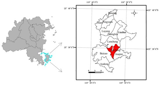
Figure 1.
Fuzhou City (left), the administrative division of Pingtan (right) (the red area is the city center).
2.2. Data Sources and Processing
Landsat 8 OLI remote sensing image data from the US Geological Survey website (https://glovis.usgs.gov/, accessed on 10 August 2022), which includes 11 bands with a resolution of 30 m. The three scenarios of 23 April 2013, 2 April 2017, and 28 March 2021 were selected and processed by ENVI software. Pre-processing includes atmospheric correction and radiation calibration and so on. Because water can cause errors in the humidity index, we need to mask the water in the study area. The original images and detailed information of these three scenes are shown in Figure 2 and Table 1. Among them, the cloud cover in remote sensing images is less than 10%, and meteorological information is provided by the China Meteorological Administration (https://www.cma.gov.cn/, accessed on 20 August 2022). Overall, the imaging conditions of these three images are similar and are less affected by factors such as weather conditions.
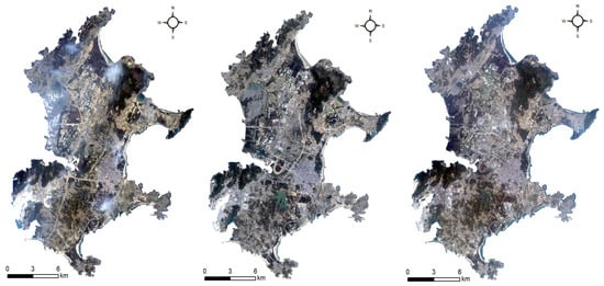
Figure 2.
Original remote sensing image in 2013, 2017, and 2021 (RGB three bands).

Table 1.
Detailed information of the three scene images.
In terms of independent variable factors, the land cover type data use the 2020 land cover type data of the global public good of geographic information (www.globallandcover.com, accessed on 3 September 2022). The land cover types in the study area consisted of eight types, namely, forestland, arable land, impervious surface, waterbody, shrubland, grassland, wetland, and bare land. Since shrubland, wetland, and bare land account for a small proportion, considering ease of analysis, the above land types are excluded in the calculation. The road data was acquired from Open Street Map (http://www.openstreetmap.org, accessed on 1 October 2022), and the demographic data were derived from open spatial demographic data and research (https://www.worldpop.org, accessed on 3 October 2022), with a resolution of 100 m × 100 m. Using the regional statistics module of ArcGIS software, taking a 500 m × 500 m regular grid as a reference unit, the RSEI value, percentage of land cover type, road density, and population density of each cell grid were counted as a sample for subsequent spatial pattern analysis use.
3. Methods
3.1. Remote Sensing Ecological Index Extraction
The remote sensing ecological index () is composed of four indicators, including greenness, humidity, dryness, and heat. These indicators can effectively monitor and evaluate ecological conditions. Specific indicators include the vegetation index () [20], humidity index () [21], dryness index () [22,23], heat index () [24]. The four component calculation formula are listed below (Table 2).
Table 2.
Formula and reference of the four ecological indicators.
To ensure dimensional consistency, we normalized these indicators and controlled the range of indicator values from 0 to 1. The normalized formula is presented below:
In the formula, represents the normalized value of a certain index, represents the value of a particular index pixel , is the highest value of the index, and is the lowest value of the index.
Finally, the index is generated by the principal component analysis method (PCA), and the initial remote sensing ecological index is the first component in the output result. To make it easier to measure and compare the index, normalizing is also necessary. The normalization formula is as shown. Its value is between 0 and 1. All normalization processes involved in this experiment were completed by loading custom functions into ArcGIS.
3.2. Analysis of Spatial Pattern Changes
Exploratory spatial data analysis (ESDA) is an important verification method in spatial data analysis. This method can accurately determine whether there is a spatial autocorrelation relationship between regions [26] to reveal the spatial aggregation and abnormality of the RSEI. This paper analyses the spatial pattern changes of the RSEI from global and local Moran index models.
The global Moran index formula can be expressed as [27]:
where and are the values of grids and , is the average value of the , is the spatial weight between elements and , and is the total number of grids in the study area. The value of is usually −1 (negative spatial autocorrelation) to 1 (positive autocorrelation), and zero means that there is no spatial autocorrelation [28].
The global Moran indicator cannot directly display the aggregation of regions. Therefore, the spatial correlation local index (LISA) is further used to evaluate the local spatial correlation and indicate the importance of hot and cold spots. The local Moran index formula could be written as [29]:
The local Moran index is a statistical method used to measure spatial data aggregation patterns, which can help us understand the spatial distribution of data. In local Moran results, there are usually four aggregation modes: High-High, High-Low, Low-Low, and Low-High cluster. These patterns can help us understand the local features of spatial data. Among them, High-High clustering refers to the clustering pattern between features with similarly high values within a certain region, indicating that in areas with particularly good ecological quality, the surrounding areas may be affected by it, and the ecological quality is also good. Likewise, Low-Low clustering refers to the clustering pattern between features with similarly low values within a certain region. It indicates that in areas with poor ecological quality, the ecological environment in the surrounding areas may also be affected by it.
3.3. Analysis of Influencing Factors
The regression analysis of influencing factors is divided into three steps. First, the least-squares regression (OLS) model is used for global modeling to obtain the preliminary evaluation results pertaining to the influence of factors on the ecological condition. The dependent variable of the model is based on the mean value of the RSEI in each grid. The selection basis of independent variables is as follows: Urban ecosystem is an ecosystem formed by the interaction of human, natural, and artificial factors, and there are various factors that will affect the urban ecosystem, mainly including urbanization, urban pollution, buildings and infrastructure, climate change and human activities. Considering the small size of the research area in this article and the difficulty in obtaining refined data due to grid division, combined with previous studies, the urban ecological environment is significantly influenced by land use [30]. Road density is one of the most common and important human interference factors among many urban landscape factors [31]. Population density is strongly correlated with the ecological condition, and population growth puts pressure on resources and the environment, which will change the landscape of sustainable environmental development [32]. Based on the above considerations, this article ultimately selected variables closely related to urbanization and human activities such as land use, road density, and population density as the independent variables for the experiment. The calculation formula of the OLS model can be expressed as:
where is the value of the dependent variable, is the intercept, is the value of the - independent variable at the - point, is the slope or regression coefficient of the - independent variable, and is the residual.
Since the regression coefficients obtained by the OLS model are the fitting results of the overall sample of the current study area, they cannot reflect the differences and changes of the impact factors on the spatial scale. It is necessary to further introduce the GWR model. The GWR equation could be written as:
where is the value of the dependent variable, is the spatial position of the - point, is the value of the continuous function at point , and is the error.
The GWR method offers benefits to the regression modeling process by considering spatial variations and assuming a constant spatial scale over the entire area of interest. Nevertheless, in situations where multiple spatial processes with different spatial scales are present, a fixed spatial scale may not be appropriate. In such cases, MGWR allows for a spatially-varying relationship between the response variable and explanatory variables, incorporating different bandwidths over the surface of the study area. Essentially, the MGWR model offers more flexibility in accounting for the complexities of spatially varying relationships and the MGWR is as:
The parameters used in MGWR are almost identical to those in GWR, except for the variable bandwidths, which are denoted by the label of , which refers to the different bandwidths assigned to each variable.
4. Results
4.1. Experimental Data Analysis
Based on the research method proposed in this paper, the RSEI of the three phases of remote sensing images is first obtained. Table 3 and Table 4 show the minimum, maximum, and standard deviation of the four ecological indices and RSEI before normalization. From Table 5, it can be seen that the RSEI of the research area has been on the rise during 2013–2021. From the perspective of the PC1 load of each ecological index, among the greenness and humidity indicators that have a positive effect on the ecology, greenness has a higher contribution rate, indicating that vegetation has a noticeable effect on enhancing the ecological conditions. while the degree index of heat and dryness is not conducive to the ecology, which is in line with the facts. In addition, the PC1 load of the greenness and humidity indicators showed a downtrend from 2013 to 2021, indicating that the contribution of both decreased year by year among the four indicators. While the PC1 load of the heat and dryness indicators increased first and then decreased, their contribution was also in the same trend.
Table 3.
Four ecological indices before normalization in different years.
Table 4.
Remote sensing ecological index before normalization in different years.
Table 5.
Four ecological indices and remote sensing ecological indices in different years.
In this experiment, the average value of RSEI was selected for subsequent experimental analysis. By dividing the RSEI into five categories at equal intervals of 0.2, the corresponding ecological environment is excellent, good, moderate, fair, and poor in 5 levels, and poor indicates the worst ecological quality, while excellent indicates the best ecological quality. Figure 3 displays the variations in the spatial pattern of ecological index classifications from 2013 to 2021. It can be seen from the figure that compared with 2013, the primary cause for the enhancement of the overall ecological condition of the study area is that the areas of poor (0–0.2) red and fair (0.2–0.4) orange grades have been significantly reduced, and the locations are mostly concentrated in the western, eastern, and central regions, corresponding to the blue, purple, and yellow boxes in Figure 3. Areas and other new development zones with a high intensity of land change, such as the southwest port economic and trade zone (the blue box) and the northwest reclamation area (the red box), are largely affected by man-made development activities. The reasons for the above-mentioned regional ecological improvement are largely related to the greening measures of relevant government departments. The original bare land is replaced by large-scale artificial vegetation greening, which makes the ecological situation better year by year; on the other hand, there are larger areas with a high ecological quality, primarily located in the northern high-altitude mountainous areas, which are less affected by human activities and have high vegetation coverage.
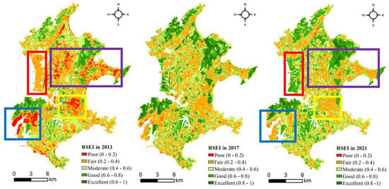
Figure 3.
Spatial distribution of RSEI in 2013, 2017, and 2021.
4.2. RSEI Spatial Autocorrelation Analysis Based on LISA
The spatial pattern of the RSEI was further investigated using the Moran index, and the findings indicated that the RSEI in the research region has obvious spatial autocorrelation. Among them, Moran’s I index in 2013 was 0.653, and the value was 41.253. In 2017 and 2021, Moran’s I index and the values were 0.596, 0.649, and 37.677, 41.036 respectively. The values are all higher than the critical value of 1.96 [33], indicating that it passed the test at the 95% significance level.
To visually depict the spatial distribution pattern of remote sensing ecological quality in Pingtan Country, the spatial characteristics of grid cells were further analyzed through the local Moran index, and the spatial distribution map of Figure 4 was drawn. Among them, the mountains situated in the north and southwest corners of the area contained the H-H area with a superior ecological environment, while the low-low (L-L) area with poor ecological quality is concentrated in the old city in the east, and the new area in the southwest. In the development zone, the reclamation area in the west with the most obvious difference in clustering characteristics between the two phases changed from the LL cluster area in 2013 to HH (the area outlined in red in Figure 4), which plays a key role in the improvement of the overall ecological environment.
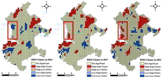
Figure 4.
Significant clusters of RSEI in 2013, 2017, and 2021 (the red box represents the most significant cluster change area in RSEI).
4.3. RSEI Spatial Heterogeneity Analysis Based on OLS, GWR, and MGWR
The OLS, GWR model, and MGWR model are used to study the correlation between the ecological environment and the three influencing factors of land cover type, road density, and population density. The fitting accuracy of the model uses and as evaluation indicators. The fitting results of the model are shown in Table 6. It should be noted that when constructing the MGWR model, only the RSEI value from 2021 was selected as the dependent variable, without considering temporal changes.
Table 6.
Fitting statistics of the models.
The global OLS model demonstrates the lowest (0.64) and the largest (2129.924), which indicates this model has certain limitations in reflecting the differences and changes of the influencing factors on the whole study area’s spatial scale. On the contrary, the GWR and MGWR models show great superiority in exploring the local spatial differentiation in connection with the urban ecological quality, the of both models increased to 0.851 and 0.882, respectively, and the greatly decreased. The data fitting effect of the MGWR model is better than other models as a whole, and its indicators are optimal.
5. Discussion
5.1. Analysis of OLS Model Coefficient
To compare how various factors affect the RSEI, the factors were standardized to eliminate the influence of dimensions. Table 7 shows the regression coefficients of the OLS model. Among them, the regression coefficient of the forest is 0.578, indicating that forestland and RSEI are positively correlated, and the positive effect is the most significant; in contrast, the regression coefficients of cropland, impervious surface, road density, and population density are negative, indicating that these variables are negatively correlated with RSEI. This is the same as the conclusions of some previous studies on the ecological environment based on cities [34]. Among them, the negative correlation of impervious surfaces is the most obvious, and its value is −0.210. Grassland types have a significance level p-value greater than 0.05, indicating that have no significant impact on RSEI.
Table 7.
Model coefficient estimates of the global model.
The global OLS model used to analyze the relationship between urban ecological quality and explanatory variables across Pingtan Island yielded a low value of 0.64. This suggests that 36% of the variability in urban ecological quality is not accounted for by the explanatory variables and may be due to other unknown factors. As a result, the OLS model’s assumption of a constant relationship across space is insufficient to fully capture the underlying relationship.
5.2. Analysis of GWR and MGWR Model
Since the establishment of Pingtan Comprehensive Experimental Zone in 2010, the construction and development of beach islands have entered a rapid development stage. At present, the development stage mainly includes three major regions: the Central business district in the central region, the Port economic district in the southwest, and the Science and technology district in the northern regions. The main layout is shown in Figure 5.
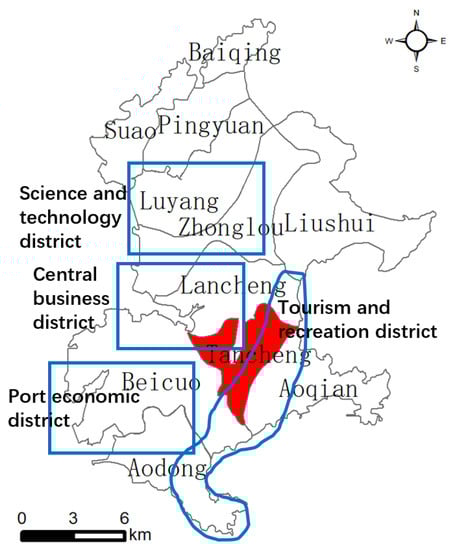
Figure 5.
Main layout plan of Pingtan (the red area is the city center, the blue frames correspond to different functional zones in Pingtan).
To investigate the spatial variability in the relationship between the predictors and urban ecological quality, both GWR and MGWR were utilized using identical variables as the global models. The diagnostic measures for GWR showed that the and were relatively improved. By using an optimal bandwidth of 1016.220, the increased to 0.851, and the decreased to 1418.673, which was much smaller than the of the global model (2129.924), suggesting a more appropriate fit. Nevertheless, the MGWR model demonstrated the highest (0.882) and the lowest (1299.883) among all of the fitted models.
The significant variables’ coefficients for GWR and MGWR are visualized in Figure 6 and Figure 7, respectively. The proportion of arable land is an influencing factor in explaining changes in ecological indicators. This variable represents a more similar pattern in describing the spatial distribution of ecological indices in GWR and MGWR. From the estimation of the coefficient of cultivated land ratio, the ecological indicators of the northern, eastern, and southern regions of the research region were negatively correlated, which reveals that the increase of cultivated land ratio in this area was not conducive to ecological quality. It can be found that in the urban planning of Pingtan Island, these areas mainly develop tourism and pay more attention to protecting the ecological environment, which may be related to agricultural development limiting ecological development to some degree. For the area under investigation’s western region, the GWR and MGWR models had poor predictability and a small proportion of arable land, which were statistically positively correlated with ecological indicators.
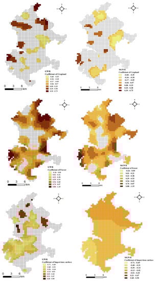
Figure 6.
The effects of the proportion of land-use types, covering Cropland (above), Forest (middle), and Impervious surface (below) in describing urban ecological quality using GWR (left) and MGWR (right) models throughout the Pingtan Island.
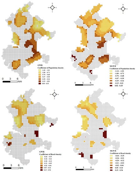
Figure 7.
The impacts of Road density (above) and Population density (below) on urban ecological quality are shown in the GWR (left) and MGWR (right) models across Pingtan Island.
The estimated coefficients for the proportion of forest exhibit spatial variation throughout the study area, as shown in Figure 6. Both models indicate that this variable behaves similarly in explaining the distribution state of ecological indices. The regression coefficients of forest land were positive, indicating that the influence of forest land on the remote sensing ecological index was mainly positive. In addition, the regression coefficient of forest land showed a decreasing trend centered on the northeast, southwest, and central regions, indicating that in these areas, the increase in the proportion of forest land type would have a more significant effect on improving the ecological environment. These areas are key areas for urban economic, commercial, and technological development, which may be related to the government’s strong implementation of green policies to protect the ecological environment while developing these areas. These policies have had a positive impact on ecology.
The impervious surface ratio was the variable with the most significant negative correlation among all independent variables, and the influence of impervious surface ratio on RSEI was significantly inconsistent between GWR and MGWR models. In MGWR, the impervious surface showed a trend of decreasing from the northern region to the southern region, indicating that the impervious surface had a higher impact on RSEI in the northern region than in other regions, this may be related to the vigorous construction of technology industry zones and central business districts in the northern and central regions of Pingtan Island in recent years. Moreover, the regression coefficients of impervious surfaces are all negative, implying that impervious water has only negative effects on the influence of ecological quality, and the increase of impervious surfaces will lead to a decrease in RSEI when other conditions remain unchanged.
According to Figure 7, the models show that demographic density is a significant predictor of the spatial pattern of ecological conditions in the research region. The GWR coefficient map reveals a spatial pattern of negative coefficient estimates that decrease from the center of the study area toward the periphery. The ecological index in these areas shows a strong negative correlation with population density. Similarly, The MGWR coefficient map reveals that there are differences in the coefficient estimates across various locations within the study area. In general, in the study area’s northern region, there are negative coefficient estimates that are relatively small, suggesting a weaker correlation between population density and urban ecological quality. Conversely, larger population estimates located at the heart of the study area are associated with a lower ecological index, suggesting that higher population density leads to lower ecological quality. Considering that the central area is the old urban area of Pingtan, with an extensive residential populace and a significant level of urbanization, the ecological index is relatively low.
The GWR and MGWR coefficient outcomes for road density are also displayed in Figure 7, which manifest a high degree of agreement in spatial structure. A series of negative coefficient values were located in the northern part of the investigation region. With the exception of a portion of the central district, most of the regression coefficients were negative, and the effect of road density on RSEI was negative in the overall study area, indicating that road density covariates explained the urban ecological index. There is a higher ecological index at lower road density when other conditions remain unchanged. Considering that the negative coefficient values are mainly concentrated in the northern region of the research area, this might be associated with Pingtan’s additional expansion of urban road infrastructure while developing the science, technology, culture, and education zone.
Figure 8 reveals the spatial heterogeneity of the fit within the study area, which is reflected in the spatially variable local of the GWR and MGWR models. It can be found that the GWR and MGWR models demonstrate a high degree of consistency, especially in the northern, north-eastern, and south-western regions of the study area, which can predict accurately and explains local relationships better ( > 0.7). Spatially there is a decreasing outward trend from the centers of these areas, considering that the larger local distribution pattern is associated with land-use types, which are identified by a larger percentage of forest land and a lower percentage of arable land. Throughout the northwest region of the study area, the local value remained consistently low ( < 0.5), indicating a weak model match. This is likely owing to notable local variability in both spatial land use and demographic traits.
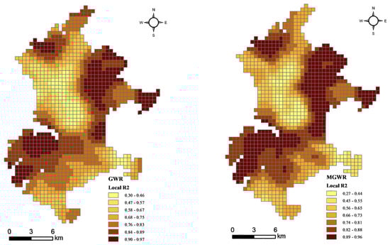
Figure 8.
Spatial pattern of local of GWR (left) and MGWR (right) models for urban ecological quality related to the important covariates throughout the Pingtan Island.
Table 8 presents an overview of the statistical measures for the coefficients of MGWR at the local level. The OLS model generated spatial distributions that were less varied and more generalized, which could limit the accuracy of estimates for ecological quality. In contrast, the GWR and MGWR models provided more precise approximations by taking local characteristics and spatial heterogeneity into consideration.
Table 8.
Model coefficient estimates of the MGWR model.
The research utilized the MGWR software to generate both GWR and MGWR results, using the golden section bandwidth searching method. This software was created by Charlton, B., Fotheringham, A. S., Brunsdon, C., & Li, J. and originating from Arizona, USA. The findings indicate that while both GWR and MGWR improve upon the results of OLS, MGWR shows a higher level of fitness. In applying the MGWR method, a cross-validation process was used to determine the number of grids necessary for solving the local regression model structure. was then utilized to adaptively select the optimal number. Both GWR and MGWR models employed Fixed Gaussian kernel function methods. Additionally, the local models’ adjustment resulted in an optimal bandwidth matrix (Table 9), which serves as the model operation’s spatial scope.
Table 9.
Multiscale bandwidth of local models GWR and MGWR.
Based on the optimal bandwidth results for each variable, the variables are categorized based on their scope or extent, with consideration of their local, regional, or global impact. Compared with the local bandwidth scale shown by the GWR model of 1016.22, MGWR supposes that the bandwidth ranges from 570.42 to 5725.35 (Table 9). The results indicate that the bandwidth of arable land and forest is relatively small, with values of 543.340 and 1034.650, respectively, indicating that this variable affects the local urban ecological quality, and is therefore categorized as a variable that operates or has an effect primarily at the local level. The bandwidth of impermeable surfaces and population density is 1891.360 and 2760.250, respectively, indicating that these variables have relatively large spatial scales, which we define as regional scale variables; road density is more significant globally, and this result is closely related to the strong connectivity of roads in cities.
In summary, the global models were found to be insufficient in representing the observed spatial variation, while the local models (GWR and MGWR) showed a higher level of goodness-of-fit and could recognize the specific patterns present in a local area more accurately. Of the two, MGWR offered the most comprehensive and suitable match. In addition, in comparison to solely utilizing GWR, the use of MGWR proved to be more effective in modeling the spatial variation in ecological quality at local geographic scales.
6. Conclusions
This paper used Landsat 8 remote sensing images as the data source and adopted RSEI and GIS spatial analysis methods to evaluate the regional pattern and influencing factors of the ecological environment in Pingtan. The research findings revealed the overall ecological condition of the research region has been significantly enhanced during 2013–2021, and the main contribution was that the vegetation coverage of the new western development area has been significantly improved. Through global and local spatial autocorrelation analysis, it can be seen that the RSEI index has an obvious spatial clustering phenomenon, which is prominent in that the high-high clusters gradually expand to the city edge, while the low-low clusters are concentrated in the city center, indicating that urban ecological development is a spatial pattern closely related to urban boundaries.
Furthermore, according to OLS, GWR, and MGWR models, the influence relationship between land use ratio, road density, population density, and RSEI in the study area was studied. The OLS model can obtain preliminary evaluation results of the effect of independent variables on the urban environmental ecology, for instance, the increase in road and population density will lead to a decrease in RSEI, while an increase in the proportion of forestland coverage will lead to an increase in RSEI. However, the OLS model is inadequate in fully representing the perceived spatial variations. The GWR model could reflect spatial changes at a constant spatial scale, but considering that complex land use types, roads, and population factors related to urban ecological quality may vary at different scales, for example, the bandwidth of all independent variables in the GWR model is 1016.22, which is considered a local scale variable. On the contrary, MGWR can reflect the changes in urban ecological quality and independent variables at different spatial scales. Cultivated land and forest land are considered to act on a local scale, indicating that these two variables affect the local urban ecological quality and will form a smaller range of urban radiation. Impervious surface and population density are considered regional variables, indicating that these variables affect urban ecological quality on a relatively large spatial scale. Road density is seen as affecting the ecological quality of cities on a global scale. Therefore, MGWR is considered a model that can cover real local patterns and more accurately reflect changes in urban ecological quality. Therefore, MGWR is considered a model that can cover real local patterns and more accurately reflect changes in urban ecological quality. The model is more suitable for urban areas with obvious spatial heterogeneity of ecological quality changes and can provide scientific references for ecological planning and ecological environment construction.
The rapid development of coastal cities has led to increasingly obvious problems such as reclamation and illegal land abuse. Pingtan, as a national comprehensive experimental area, is representative of the assessment of its ecological environmental changes. For the study area in this article, we provide the following suggestions for the future stable and sustainable advancement of the urban economy and ecosystem in the study area: (1) Changes in land cover types and changes in road density have an important impact on the development of urban ecological quality. Compared with the more complex mountainous areas, the plain areas are more affected by human factors, and the ecological environment is easily affected. In the future, urban construction needs to focus on ecological protection. (2) Forestland affects improving the quality of the ecological environment. In urban construction, protection measures such as building parks and public green spaces at all levels in the city should be increased. (3) For island cities, efforts should be made to strengthen coastal ecological construction and environmental protection, such as improving coastal shelter forest construction, increasing the types of shelter forest trees, and protecting tidal flat wetland ecosystems.
This article considers the land-use type, road density, and population density in the selection of image elements and explores the relationship between them and ecological quality. The limitation of this paper is that in the MGWR model, the analysis of spatial heterogeneity between independent variables and RSEI does not consider the impact of time series, but only the model analysis between RSEI and independent variables in 2021. Subsequent research will consider increasing the time dimension. The specific solutions are as follows: firstly, using the difference between RSEI years to analyze its relationship with independent variables; secondly, collecting independent variable data for each year’s RSEI value for model analysis. However, considering the difficulty of data collection, future research direction is more inclined toward the first option. In addition, due to the small scope of the research area selected in this article, and considering the limitations and difficulties of data collection, future research directions will focus more on research and analysis in larger cities or multiple regions.
Author Contributions
The manuscript was primarily written by P.Y., who also designed and conducted the comparative experiments; X.Z. provided supervision throughout the study and reviewed and edited the manuscript; L.H. contributed to the manuscript by providing comments and suggestions for improvement, and also assisted with revisions. All authors have scanned and approved the final draft for publication. All authors have read and agreed to the published version of the manuscript.
Funding
This project received funding from the National Natural Science Foundation of China (62103345) and the Science and Technology Planning Project of Fujian Province (2020H0023, 2020J02160, 2020J01265).
Data Availability Statement
The remote sensing image data of Landsat 8 OLI comes from the website of the United States Geological Survey (https://glovis.usgs.gov/, accessed on 10 August 2022). We selected three scenarios: 23 April 2013, 2 April 2017, and 28 March 2021. The land cover type data use the 2020 land cover type data of the global public good of geographic information (www.globallandcover.com, accessed on 3 September 2022), with a resolution of 30m. The road data was acquired from Open Street Map (http://www.openstreetmap.org, accessed on 1 October 2022), and the demographic data were derived from open spatial demographic data and research (https://www.worldpop.org, accessed on 3 October 2022), with a resolution of 100 m.
Acknowledgments
We would like to express our appreciation to the reviewers, whose insightful and constructive comments were highly valuable to improving the quality of our work on previous versions of this document. The authors also want to thank editors for their patient and meticulous work for our manuscript.
Conflicts of Interest
The authors declare no conflict of interest.
References
- Xu, H.; Wang, M.; Shi, T.; Guan, H.; Fang, C.; Lin, Z. Prediction of Ecological Effects of Potential Population and Impervious Surface Increases Using a Remote Sensing Based Ecological Index (RSEI). Ecol. Indic. 2018, 93, 730–740. [Google Scholar] [CrossRef]
- Zhou, W.; Qian, Y.; Li, X.; Li, W.; Han, L. Relationships between Land Cover and the Surface Urban Heat Island: Seasonal Variability and Effects of Spatial and Thematic Resolution of Land Cover Data on Predicting Land Surface Temperatures. Landsc. Ecol. 2014, 29, 153–167. [Google Scholar] [CrossRef]
- Lin, T.; Ge, R.; Huang, J.; Zhao, Q.; Lin, J.; Huang, N.; Zhang, G.; Li, X.; Ye, H.; Yin, K. A Quantitative Method to Assess the Ecological Indicator System’s Effectiveness: A Case Study of the Ecological Province Construction Indicators of China. Ecol. Indic. 2016, 62, 95–100. [Google Scholar] [CrossRef]
- Xu, H. A Remote Sensing Urban Ecological Index and Its Application. Shengtai Xuebao Acta Ecol. Sin. 2013, 33, 7853–7862. [Google Scholar]
- Firozjaei, M.K.; Fathololoumi, S.; Weng, Q.; Kiavarz, M.; Alavipanah, S.K. Remotely Sensed Urban Surface Ecological Index (RSUSEI): An Analytical Framework for Assessing the Surface Ecological Status in Urban Environments. Remote Sens. 2020, 12, 2029. [Google Scholar] [CrossRef]
- Wang, C.; Jiao, L.; Lai, F.; Zhang, N. Ecological Change Evaluation of Manas Lake Wetland in Xinjiang Based on Remote Sensing Ecological Index. Shengtai Xuebao Acta Ecol. Sin. 2019, 39, 2963–2972. [Google Scholar]
- Wang, S.; Zhang, X.; Zhu, T.; Yang, W.; Zhao, J. Assessment of ecological environment quality in the Changbai Mountain Nature Reserve based on remote sensing technology. Prog. Geogr. 2016, 35, 1269–1278. [Google Scholar]
- Wen, X.; Lin, Z.; Tang, F. Remote Sensing Analysis of Ecological Changes Caused by the Construction of Emerging Island Cities: A Case Study of Pingtan Comprehensive Experimental Zone in Fujian Province. Appl. Ecol. Sci. 2015, 26, 541–547. [Google Scholar]
- Carroll, M.C.; Reid, N.; Smith, B.W. Location Quotients versus Spatial Autocorrelation in Identifying Potential Cluster Regions. Ann. Reg. Sci. 2008, 42, 449–463. [Google Scholar] [CrossRef]
- Yang, Y.; Wong, K. Spatial Distribution of Tourist Flows to China’s Cities. Tour. Geogr. 2013, 15, 338–363. [Google Scholar] [CrossRef]
- Anselin, L. Lagrange Multiplier Test Diagnostics for Spatial Dependence and Spatial Heterogeneity. Geogr. Anal. 1988, 20, 1–17. [Google Scholar] [CrossRef]
- Brunsdon, C.; Fotheringham, S.; Charlton, M. Geographically Weighted Regression. J. R. Stat. Soc. Ser. Stat. 1998, 47, 431–443. [Google Scholar] [CrossRef]
- Curt, T.; Bouchaud, M.; Agrech, G. Predicting Site Index of Douglas-Fir Plantations from Ecological Variables in the Massif Central Area of France. For. Ecol. Manag. 2001, 149, 61–74. [Google Scholar] [CrossRef]
- Louw, J.H.; Scholes, M. Forest Site Classification and Evaluation: A South African Perspective. For. Ecol. Manag. 2002, 171, 153–168. [Google Scholar] [CrossRef]
- Fotheringham, A.S.; Yang, W.; Kang, W. Multiscale Geographically Weighted Regression (MGWR). Ann. Am. Assoc. Geogr. 2017, 107, 1247–1265. [Google Scholar] [CrossRef]
- Hastie, T.; Tibshirani, R. Generalized Additive Models: Some Applications. J. Am. Stat. Assoc. 1987, 82, 371–386. [Google Scholar] [CrossRef]
- Li, B.; Shi, X.; Wang, H.; Qin, M. Analysis of the Relationship between Urban Landscape Patterns and Thermal Environment: A Case Study of Zhengzhou City, China. Environ. Monit. Assess. 2020, 192, 540. [Google Scholar] [CrossRef]
- Yuan, W.; Sun, H.; Chen, Y.; Xia, X. Spatio-Temporal Evolution and Spatial Heterogeneity of Influencing Factors of SO2 Emissions in Chinese Cities: Fresh Evidence from MGWR. Sustainability 2021, 13, 12059. [Google Scholar] [CrossRef]
- Fotheringham, A.S.; Yue, H.; Li, Z. Examining the Influences of Air Quality in China’s Cities Using Multi-Scale Geographically Weighted Regression. Trans. GIS 2019, 23, 1444–1464. [Google Scholar] [CrossRef]
- Goward, S.N.; Xue, Y.; Czajkowski, K.P. Evaluating Land Surface Moisture Conditions from the Remotely Sensed Temperature/Vegetation Index Measurements: An Exploration with the Simplified Simple Biosphere Model. Remote Sens. Environ. 2002, 79, 225–242. [Google Scholar] [CrossRef]
- Baig, M.H.A.; Zhang, L.; Shuai, T.; Tong, Q. Derivation of a Tasselled Cap Transformation Based on Landsat 8 At-Satellite Reflectance. Remote Sens. Lett. 2014, 5, 423–431. [Google Scholar] [CrossRef]
- Rikimaru, A.; Roy, P.S.; Miyatake, S. Tropical Forest Cover Density Mapping. Trop. Ecol. 2002, 43, 39–47. [Google Scholar]
- Xu, H. A New Index-Based Built-up Index (IBI) and Its Eco-Environmental Significance. Remote Sens. Technol. Appl. 2011, 22, 301–308. [Google Scholar]
- Wang, F.; Qin, Z.; Song, C.; Tu, L.; Karnieli, A.; Zhao, S. An Improved Mono-Window Algorithm for Land Surface Temperature Retrieval from Landsat 8 Thermal Infrared Sensor Data. Remote Sens. 2015, 7, 4268–4289. [Google Scholar] [CrossRef]
- Zhou, J.; Liu, W. Monitoring and Evaluation of Eco-Environment Quality Based on Remote Sensing-Based Ecological Index (RSEI) in Taihu Lake Basin, China. Sustainability 2022, 14, 5642. [Google Scholar] [CrossRef]
- Hu, X.; Hong, W.; Qiu, R.; Hong, T.; Chen, C.; Wu, C. Geographic Variations of Ecosystem Service Intensity in Fuzhou City, China. Sci. Total Environ. 2015, 512, 215–226. [Google Scholar] [CrossRef]
- Hu, X.; Xu, H. A New Remote Sensing Index for Assessing the Spatial Heterogeneity in Urban Ecological Quality: A Case from Fuzhou City, China. Ecol. Indic. 2018, 89, 11–21. [Google Scholar] [CrossRef]
- Peng, J.; Xie, P.; Liu, Y.; Ma, J. Urban Thermal Environment Dynamics and Associated Landscape Pattern Factors: A Case Study in the Beijing Metropolitan Region. Remote Sens. Environ. 2016, 173, 145–155. [Google Scholar] [CrossRef]
- Tang, Q.; Xu, W.; Ai, F. A GWR-Based Study on Spatial Pattern and Structural Determinants of Shanghai’s Housing Price. Econ. Geogr. 2012, 32, 52–58. [Google Scholar]
- Chen, X.; Xu, X.; Liu, Y. Review of Researches on Remote Sensing Monitoring and Impact on Environment of Land Use/Cover Change. Meteorol. Sci. Technol. 2005, 33, 289–294. [Google Scholar]
- Lin, Y.; Hu, X.; Zheng, X.; Hou, X.; Zhang, Z.; Zhou, X.; Qiu, R.; Lin, J. Spatial Variations in the Relationships between Road Network and Landscape Ecological Risks in the Highest Forest Coverage Region of China. Ecol. Indic. 2019, 96, 392–403. [Google Scholar] [CrossRef]
- Geng, T.; Chen, H.; Zhang, H.; Shi, Q.; Liu, D. Spatiotemporal Evolution of Land Ecosystem Service Value and Its Influencing Factors in Shaanxi Province Based on GWR. J. Nat. Resour. 2020, 35, 1714–1727. [Google Scholar]
- Yuan, Y.; Shi, X.; Niu, S.; Zhang, C.; Yan, S. A GWR-Based Study on Jincheng City Hollow Village Driving Force. Econ. Geogr. 2015, 35, 148–155. [Google Scholar]
- Wang, J.; Qian, Y.; Han, L.; Zhou, W. Relationship between Land Surface Temperature and Land Cover Types Based on GWR Model: A Case of Beijing-Tianjin-Tangshan Urban Agglomeration, China. J. Appl. Ecol. 2016, 27, 2128–2136. [Google Scholar]


Disclaimer/Publisher’s Note: The statements, opinions and data contained in all publications are solely those of the individual author(s) and contributor(s) and not of MDPI and/or the editor(s). MDPI and/or the editor(s) disclaim responsibility for any injury to people or property resulting from any ideas, methods, instructions or products referred to in the content. |
© 2023 by the authors. Licensee MDPI, Basel, Switzerland. This article is an open access article distributed under the terms and conditions of the Creative Commons Attribution (CC BY) license (https://creativecommons.org/licenses/by/4.0/).