Abstract
Global use of energy-inefficient mechanical vapor-compression air conditioning (AC) is increasing dramatically for home cooling. Direct evaporative coolers (EC) offer substantial energy savings, and may provide a sustainable alternative to AC for homes in hot, dry climates. One drawback of ECs is the potential for infiltration of outdoor air pollution into homes. Prior studies on this topic are limited by small sample sizes and a lack of comparison homes. In this study, we used aerosol photometers to sample indoor and outdoor fine particulate matter (PM2.5) from 16 homes with AC and 14 homes with EC in Utah County, Utah (USA) between July 2022 and August 2023. We observed a significantly larger infiltration factor (Fin) of outdoor PM2.5 in EC vs. AC homes (0.39 vs. 0.12, p = 0.026) during summer. Fin significantly increased during a wildfire smoke event that occurred during the study. During the wildfire event, EC homes offered little to no protection from outdoor PM2.5 (Fin = 0.96, 95% confidence interval (CI) 0.85, 1.07), while AC homes offered significant protection (Fin = 0.23, 95% CI 0.15, 0.32). We recommend additional research focused on cooling pad design for the dual benefits of cooling efficiency and particle filtration.
1. Introduction
Global increases in per capita income are fueling a surge in the residential use of mechanical vapor-compression air conditioners (AC) [1,2]. Typical AC units, which are not very energy efficient, currently dominate the global air conditioning market. This is particularly relevant in hot, arid climates such as in the Middle East where air conditioning accounts for up to 70% of building energy use [3,4]. Globally, housing accounts for approximately 30% of total energy consumption [5,6]. Due to increasing global temperatures, energy use for space heating is expected to decline by 34%, while energy use for space cooling is expected to grow by 72% by the end of the 21st century [7]. Davis et al. (2015) estimate that 70% of homes globally will have air conditioners by the year 2100, accompanied by an 83% increase in household energy use [8]. Thus, we are currently in an opportunity window to develop and promote sustainable, energy-saving alternatives to AC for residential space cooling.
One of the most promising alternatives to AC for arid and semi-arid regions are direct evaporative coolers (ECs). ECs cost less, require no chlorofluorocarbons (CFCs), and use only 20–50% of the energy required by AC units to achieve comparable cooling performance [9,10,11]. Globally, many regions with the largest AC adoption rates are in areas conducive to evaporative cooling. McNeil and Letschert (2008), for example, predict that by 2030, over 80% of homes in Mexico and over 50% of homes in Middle Eastern countries will have AC, up from approximately 20% and 25%, respectively, in 2005 [12]. In hot, dry climates, ECs have the potential to significantly reduce energy consumption associated with residential space cooling.
Evaporative cooling methods have been used from ancient times to the present day in various forms and across multiple cultures to provide efficient, low-cost residential air conditioning in hot, dry climates [13,14,15,16,17]. Direct evaporative cooling is the simplest and most common type of residential evaporative cooling in use today. ECs, also known as swamp, drip, or desert coolers, work based on the heat transfer associated with water evaporation. ECs use a low-power electric fan to pull hot, dry outdoor air across wetted cooling pads, usually made from plant fibers (e.g., aspen wood shavings) or corrugated cellulose materials [9,18,19]. As hot air moves across the wet cooling pads, liquid water in the cooler pads absorbs thermal energy from the hot outdoor air as it changes phase to become water vapor [20]. This process lowers the temperature and simultaneously increases the relative humidity of air being blown into the home [9,21]. Because they work based on the evaporation of water, ECs are most effective in regions where there is a large wet bulb depression and where the wet bulb temperature is below 21 °C [10].
One concern with EC use is the potential for the infiltration of outdoor air pollution into homes. ECs pull large volumes of outdoor air into homes, generating < 10 to over 30 air changes per hour (ACH) in residential buildings, depending on home size and EC fan speed [22,23]. In contrast, AC units typically recirculate air in the home to conserve energy and have low ACH rates. For example, homes in Houston TX (USA), where AC is commonly used during summer months, have a median ACH rate of 0.37 [24]. Thus, AC homes may provide a protective barrier against outdoor air pollution because they draw very little outdoor air into the home. ECs may also significantly dilute indoor pollution originating from household sources, such as tobacco smoke and cooking aerosols [25]. Among outdoor pollutants that may infiltrate homes, fine particulate matter (PM2.5) is a primary concern. PM2.5 exposure is associated with multiple poor health outcomes, including lung cancer, cardiopulmonary mortality, and infectious and non-infectious respiratory illnesses [26,27].
To date, there is little in the published literature on the infiltration of particulate air pollution into EC homes. Paschold et al. (2003) used a test chamber to evaluate indoor/outdoor (I/O) ratios of PM10 and PM2.5 associated with EC use without interference from household activities, such as smoking and cooking [28]. Using tap water to wet the EC cooling pads, the PM10 I/O ratios ranged from ~0.5 to 0.6, and the PM2.5 I/O ratios ranged from ~0.76 to 1.04 depending on pad type and fan speed. Li et al. (2003), in a study of 10 occupied homes in the El Paso, TX area, found I/O ratios of 0.57 and 0.63, for PM10 and PM2.5, respectively when the EC was running [23]. Both studies suggest that ECs provide some protection to residents from particle pollution, but they provide more protection from PM10 than PM2.5.
ECs offer substantial energy savings when compared to AC units in dry climates, and thus may provide a sustainable alternative to AC cooling in some regions. However, to be sustainable for human health, ECs should not put home occupants at higher risk of exposure to air pollution that infiltrates the home through the EC. Current evidence, albeit limited, suggests ECs may provide some protection from outdoor PM2.5 infiltration into homes. Data are especially limited on their effectiveness in protecting residents from wildfire smoke, with wildfires increasing in the Western U.S. over the last several decades [29,30,31]. The utility of ECs as a sustainable air conditioning option thus warrants further investigation into this topic. In this study, we aimed specifically to evaluate the I/O ratios of PM2.5 in occupied EC homes. This study builds upon prior research by increasing the sample size and using a comparison group of AC homes in the same area.
2. Materials and Methods
2.1. Study Design
The primary objective of this study was to evaluate PM2.5 infiltration into EC and AC homes in Utah County, UT (USA) during summer and winter months without interference from indoor aerosol sources. Utah County is located in the Western US, with a semiarid climate that is suited for ECs, but also susceptible to wildfire smoke events during the summer months. A secondary objective was to evaluate PM2.5 infiltration during wildfire smoke events in both EC and AC homes. Indoor and outdoor 24-h PM2.5 measurements were collected during each sampling event using aerosol photometers. We used convenience sampling to recruit homes from July 2022 to August 2023. Recruitment strategies included personal contacts, social media posts, and flyers mailed to university faculty and staff. Prospective participants completed a 13-item pre-screen questionnaire to determine eligibility. Inclusion criteria were: (1) must be a single-family home in Utah County, UT (USA); (2) must use either EC or AC air conditioning; (3) the primary home occupant must be at least 18 years old and the owner or renter of the property; (4) the primary home occupant must be able/willing to not cook, burn anything (candles/incense/fireplace, etc.), and not vacuum 3 h. prior and 24 h. during sampling; and (5) must plan to live in the home until at least 1 October 2024. Exclusion criteria were: (1) having a home occupant who smoked or vaped; (2) having guests who smoked or vaped in the home; and (3) using a humidifier, air purifier, or vaporizer.
We attempted to sample each home at least twice, once during the summer and once during the winter months. Additional effort was made to sample homes during a wildfire smoke event that occurred during the study. We used the Fire and Smoke Map on AirNow [32] to identify one wildfire smoke event, which occurred between 8 and 12 September 2022, with daily PM2.5 concentrations reaching over 25 µg/m3 at both of the Utah Division of Air Quality (UDAQ) monitors in Utah County (Figure S1). During this wildfire smoke event, we were able to conduct second visit measurements for three of the AC homes, and first visit measurements for four of the EC homes.
During each sampling visit, study personnel set up indoor and outdoor PM2.5 aerosol monitors and temperature/relative humidity meters. These instruments ran for approximately 24 h. Indoor monitors were placed in the main living area of the home away from windows and ventilation ducts. Laminated cards were hung on ovens and microwaves to remind occupants not to cook during the sampling period. Outdoor monitors were placed away from aerosol-generating sources such as clothes dryer vents. Study personnel administered a housing survey at each visit. The primary home occupant received a $50 Visa gift card for each visit to compensate for their time, and to cover the cost of meals during the 24 h sampling period. A video/photo release form was used to document permission to photograph participants’ air conditioning units. After the 24 h sampling period we confirmed with the study participant that no cooking, candle burning, or vacuuming was carried out during that 24 h sampling period. The Institutional Review Board at Brigham Young University (BYU) determined that the unit of study was the home, not the occupant(s), and thus did not require the human subjects’ research approval.
2.2. Data Collection
2.2.1. Aerosol Photometer
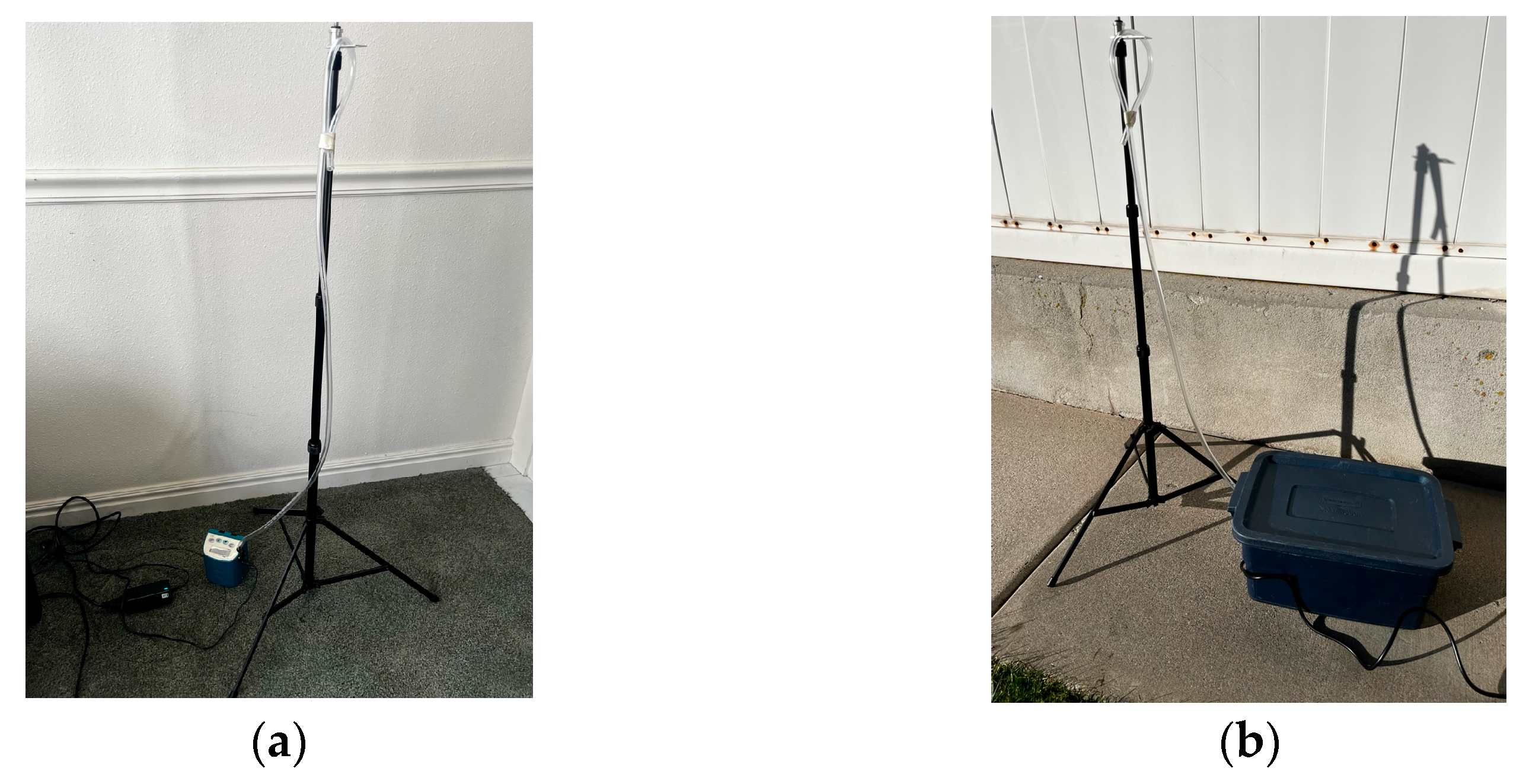
We employed SidePak AM 510 Aerosol Monitor Dataloggers (TSI Inc., Shoreview, MN, USA) to quantify the PM2.5 mass concentration in mg/m3 during each data collection visit. Prior to data collection, all SidePak instruments underwent a four-point calibration using emery oil that was nominally adjusted to respirable mass aerosol concentrations by the manufacturer per ISO 12103-1, A1 test dust (Arizona dust) [33]. We prepared the SidePak monitors as per the manufacturer’s guidelines, including downloading data from the previous visit, clearing the SidePak memory, and setting the logging interval to one minute. We cleaned and greased the impaction plate and applied grease to the impactor assembly O-ring. The flow rate was set to 1.7 lpm ± 1.0%, and the SidePak was zeroed using a HEPA filter. For both indoor and outdoor samples, the monitor was placed at the base of a tripod. Tygon® tubing was attached to the SidePak inlet and extended up to the top of the tripod 1 to 1.5 m above ground level (Figure 1a). A small loop was made with the tubing at the top of the tripod so the air inlet was facing downward. This was done to prevent water or large particles from entering the tubing. For outdoor samples, the SidePak monitor was placed in the waterproof container (Figure 1b). Data were recorded over a continuous period of approximately 24 h. SidePak monitors were connected to AC power throughout the data collection phase to ensure uninterrupted operation.

Figure 1.
Aerosol photometer tubing positioned approximately 1.0–1.5 m above the floor/ground for (a) indoor and (b) outdoor sampling. Outdoor aerosol photometers were placed in a plastic container with air holes to prevent water damage.
2.2.2. Temperature and Humidity
Extech SD500 temperature/relative humidity (TRH meters) dataloggers (Extech Instruments, Nashua, NH, USA) were used during each sample collection visit. Prior to each data collection event, previously recorded data were downloaded, the SD card was cleared, and the TRH meter batteries were replaced. The TRH meters were placed approximately 1–1.5 m off the ground on a tripod, one inside and one outside the home. The TRH meters were attached to the tripod with a piece of string. Data were logged every minute over the 24 h data collection period.
2.2.3. Demographic Data
Study personnel administered a housing survey during both the summer and winter data collection visits. The summer housing survey consisted of a 24-item questionnaire used to verify inclusion/exclusion criteria, and to collect data such as age and style of the home, number of occupants, and other housing characteristics. The questionnaire also included items regarding methods used by home occupants to ventilate the dwelling during summer months, and types of filters used in AC and EC cooling units. The winter housing survey was a 9-item questionnaire verifying inclusion/exclusion criteria and one item regarding methods used to heat the home during winter months.
2.3. Quality Assurance
We conducted quality assurance of our collected data, by reviewing and removing incomplete or suspicious data. Through our quality assurance steps, our data set was reduced from 31 homes and 67 unique home visits to 30 homes (16 AC, and 14 EC) and 50 unique home visits. Details of the data cleaning steps are included in the supplemental information.
As another data validation and quality assurance step, we compared the average PM2.5 concentrations measured from the outdoor SidePak monitors and measurements made from two Utah Division of Air Quality (UDAQ) monitors located in Utah County. Across the entire study, the outdoor PM2.5 concentrations were strongly linearly correlated between the SidePak and UDAQ monitors (R2 = 0.78). The average outdoor SidePak PM2.5 concentrations have a large systematic bias and can be more than 2× larger than the corresponding UDAQ PM2.5 concentrations (Figure S5). The light-scattering method used by the SidePak is sensitive to the particle size [34], morphology, and composition [35], as well as the temperature and humidity [36]. Our data confirmed this dependence exists in the measures collected in our study from the SidePak instruments. The slope between the outdoor SidePak PM2.5 concentrations and the closest Utah UDAQ PM2.5 concentrations is markedly different in the summer than the winter (Figures S6 and S7). Thus, the SidePak concentrations should not be used to infer absolute PM2.5 concentrations, and we need to be cautious when comparing SidePak measurements conducted under substantially different sampling conditions.
For this study, we used the raw SidePak PM2.5 measurement to evaluate the relative differences in PM2.5 concentrations (rather than absolute differences) between location (indoor and outdoor), home cooling type (AC and EC), and season (summer and winter). Others have developed and used calibration factors to adjust PM2.5 concentrations from light-scattering instruments based on relative humidity [37,38,39]. The humidity adjustments are most important at RH values of >60% [38,40]. We have chosen not to adjust the SidePak PM2.5 in our study for two reasons. First, our measurements are generally below an RH of 60% in our study (Table S4). Second, we did not collect side-by-side PM2.5 data between reference monitors and the SidePak from which to develop our calibrations.
2.4. Data Analysis
All analyses were performed using R Statistical Software (v4.3.1. R Core Team 2023). We calculated statistics from the average indoor and outdoor SidePak concentrations measured from each visit between the AC and EC homes in summer and winter. These statistics included indoor concentrations, outdoor concentrations, and indoor/outdoor ratios. We then conducted two-sample t-tests to evaluate if there are significant differences in the average statistics between the AC and EC homes within each season.
Next, we used two different methods to estimate the infiltration factor (Fin). The infiltration fraction estimates the fraction of outdoor PM2.5 that infiltrates the indoor environment and should be between 0 and 1. Under ideal circumstances where there is no source of indoor PM2.5 pollution, the I/O and Fin should be equivalent. In cases where there are indoor sources of PM2.5, Fin should be lower than the I/O ratio.
In Method 1, we estimated Fin using the correlation between the indoor and outdoor PM2.5 concentrations using the minute-by-minute SidePak measurements made at each home. We fitted a linear model to the average indoor SidePak PM2.5 concentrations for each minute, j, within each visit, I, using Equation (1), using the nomenclature consistent with Chen and Zhao (2011) [41]. We fitted the model using ordinary least squares.
where:
Cin i,j = Cs,i + Fin i Cout i,j + ei,j,
- Cin i,j = Indoor SidePak PM2.5 concentration (µg/m3) for visit, i, and minute, j
- Cs = Intercept, PM2.5 contribution (µg/m3) from indoor sources for visit, i
- Cout i = Outdoor SidePak PM2.5 concentration (µg/m3) for visit, i, and minute, j
- Fin i = Slope (infiltration factor) for visit, i
- ei,j = Error in the linear model fit for visit, i, and minute, j
In Method 2, we evaluated the correlation between the average indoor concentrations and outdoor concentrations across different visits. We estimated the infiltration factor using a linear model with the same form as in Method 1, but instead of fitting the model to the minute-by-minute data from each house visit, we fitted the model to the average indoor SidePak PM2.5 concentrations from visits grouped by air conditioning type and season, as shown in Equation (2).
where:
Cin i = Cs + Fin Cout i + ei,
- Cin i = Average indoor SidePak PM2.5 concentration (µg/m3) for visit, i
- Cs = Intercept, average PM2.5 contribution (µg/m3) from indoor sources
- Cout i = Average outdoor SidePak PM2.5 concentration (µg/m3) for visit, i
- Fin = Slope, infiltration factor
- ein = Error in the linear model fit for visit, i
3. Results
3.1. Home Demographics
Characteristics of the homes included in this study are included in Table 1. EC homes tended to be older and slightly smaller than AC homes. EC homes also tended to have fewer residents and lower occupant densities. AC homes were more likely to be owner-occupied compared to EC homes.

Table 1.
Demographics of study homes by air conditioning type.
3.2. Average Concentrations and Indoor to Outdoor Ratios
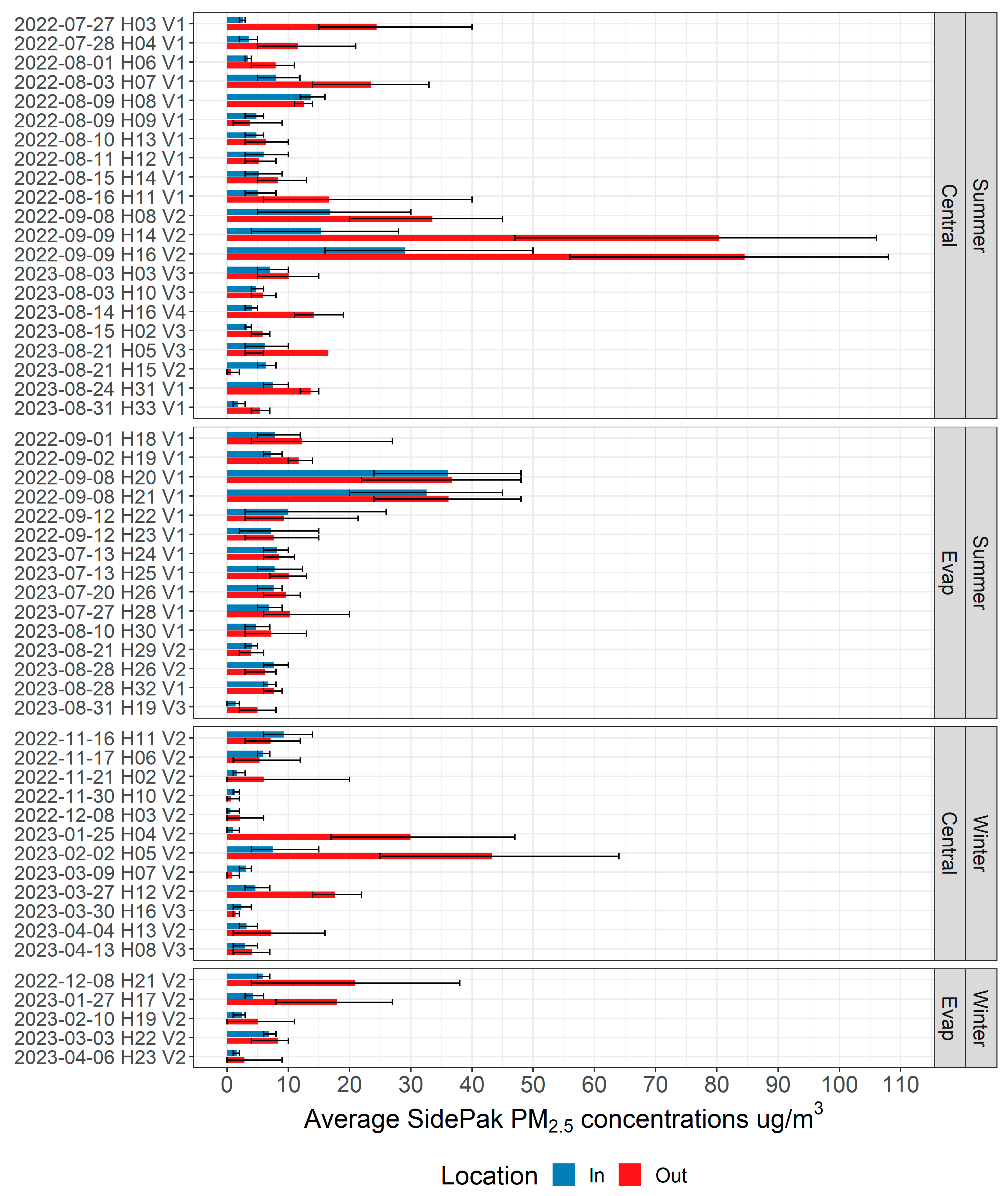
The average indoor and outdoor concentrations for the visits are displayed in Figure 2. Large variability is observed in the average outdoor concentrations across the study. Larger outdoor concentrations are observed during the wildfire event occurring from 8 to 12 September 2022. Additionally, a few high outdoor concentrations are observed during the winter months, which are attributed to inversion conditions that frequently occur in Utah County in the winter. The indoor concentrations vary considerably in the summer, but are all relatively low during the winter.
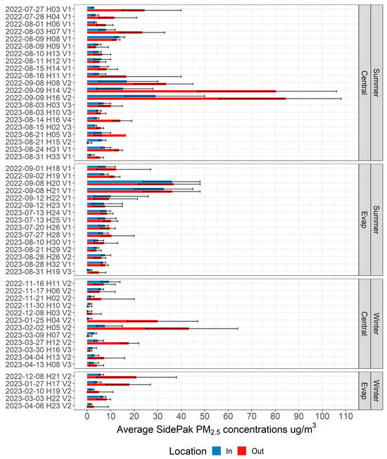
Figure 2.
Average indoor and outdoor SidePak PM2.5 concentrations for each date, home (H), and visit (V) grouped by season and air conditioner type from the final dataset. The error bars are the 10th and 90th percentile minute-by-minute concentrations for each home visit.
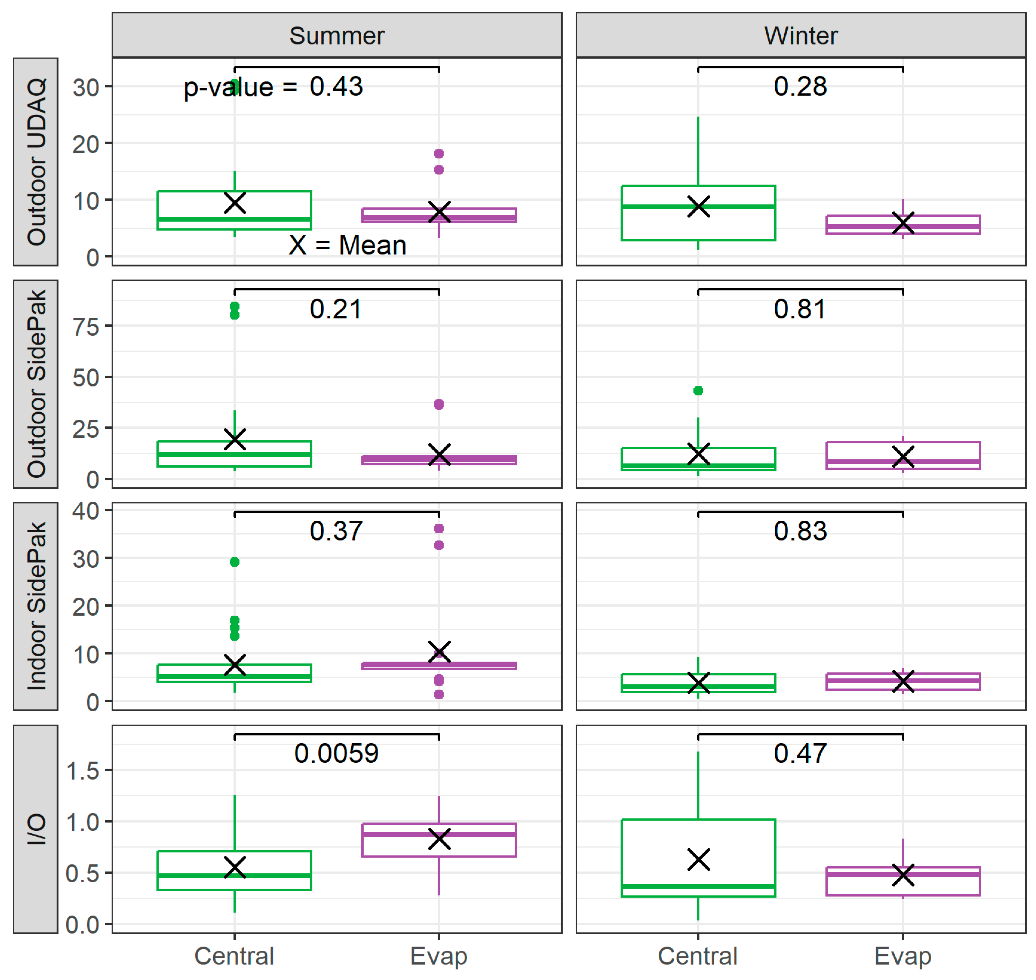
In Figure 3, we summarized the average indoor and outdoor PM2.5 concentrations measured for each home visit grouped by air conditioner type and season using box-plots. We also added the group average of the home visits by air conditioner and season. The average outdoor PM2.5 concentrations measured by the closest reference UDAQ monitor and at the home by the SidePak monitors were consistently higher in AC homes, but the difference was not statistically significant. On the other hand, the mean indoor SidePak PM2.5 concentrations were larger from the visits with EC homes for both summer and winter. For the t-tests, we treated each home visit as an independent and random variable, even though we conducted repeat visits at several of the homes during the summer season. This is a reasonable assumption, because the I/O ratios within repeated home visits have as much variability as those of visits between different homes (Figure S8).
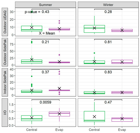
Figure 3.
Box plots of average concentration statistics from the home visits organized by air conditioner type and season; “Outdoor UDAQ” = The average outdoor PM2.5 concentrations (µg/m3) from the UDAQ reference monitors; “Outdoor SidePak” = the outdoor PM2.5 concentrations (ug/m3) from the SidePak monitors; “Indoor SidePak = the average indoor PM2.5 concentrations (µg/m3) from the SidePak monitors; “I/O” = I/O ratio calculated from the average indoor and outdoor SidePak PM2.5 concentrations. The box plots are in the style of Tukey; middle line is the median, the bottom and upper lines are the 25th and 75th percentiles, respectively; whiskers extend to the largest value within 1.5 times the interquantile range; observations beyond the whiskers are labeled individually [42]. The X symbols represent the mean group value, and horizon lines and numbers are the p-values comparing the averages from a two-sample t-test.
Figure 3 also displays the mean and the distribution of I/O ratios across each home visit using the average SidePak PM2.5 concentrations. The average I/O ratio across the summer visits was significantly higher in EC homes (0.83) than in AC homes (0.55; p-value = 0.006, See Table S11). These results are dependent on the seven home visits during the 8–12 September 2022 wildfire smoke event. When we remove the seven home visits in the summer that occurred during the wildfire smoke event, the difference in the average I/O by air conditioning type is no longer significant (p-value = 0.1, Figure S9). During the winter, the average I/O ratio across home visits is lower in EC homes, but the difference is not statistically significant.
Because we attempted to minimize indoor air pollution sources, and removed home visits that appeared to have strong indoor sources, we attribute the higher I/O ratios to a higher infiltration of outdoor air pollution in homes with evaporative coolers. In the next two sections, we empirically estimated the infiltration fraction of outdoor PM2.5, which is the fraction of the outdoor PM2.5 concentration that infiltrates the indoor environment.
3.3. Infiltration Factor Using Method 1
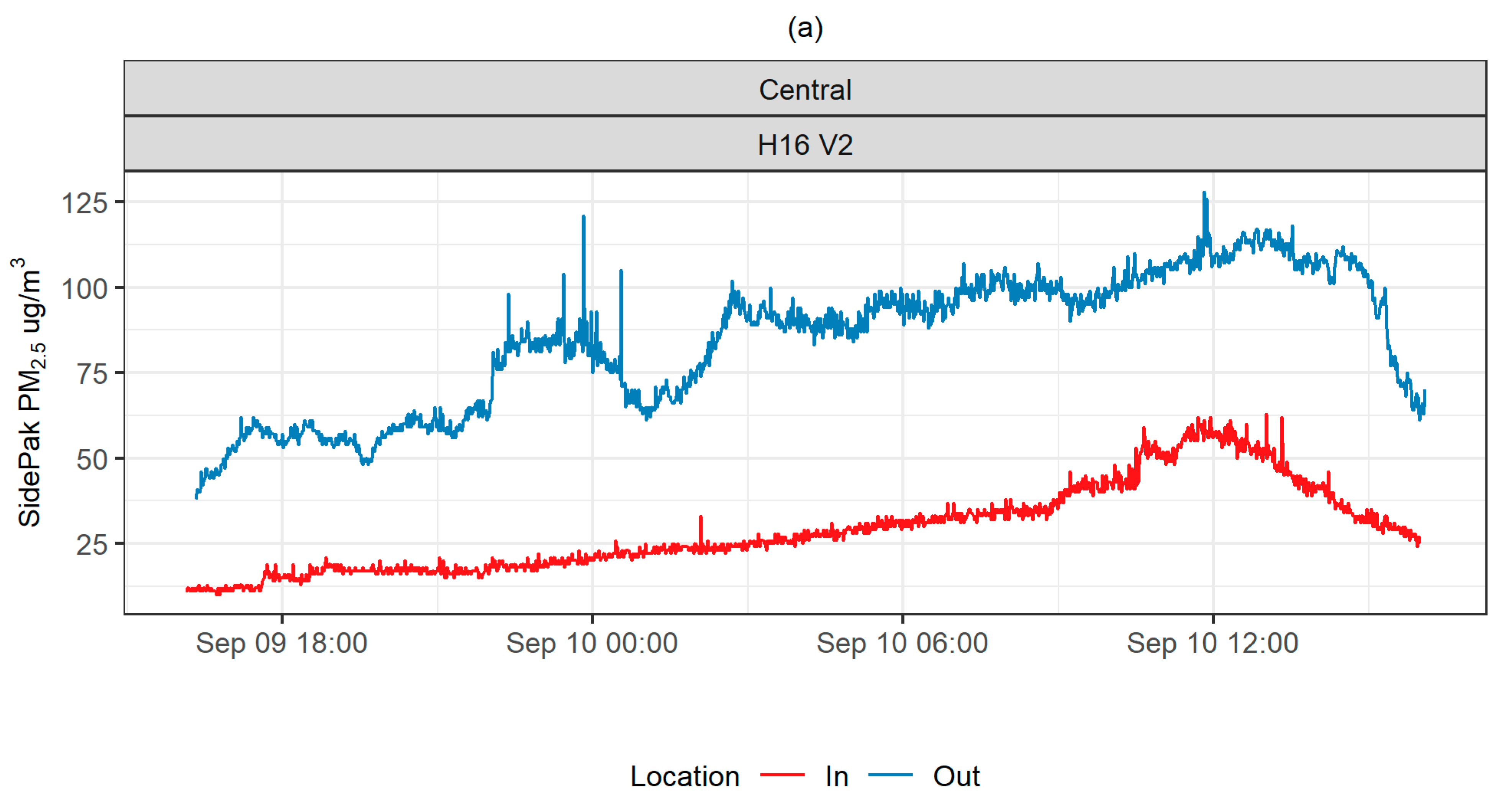
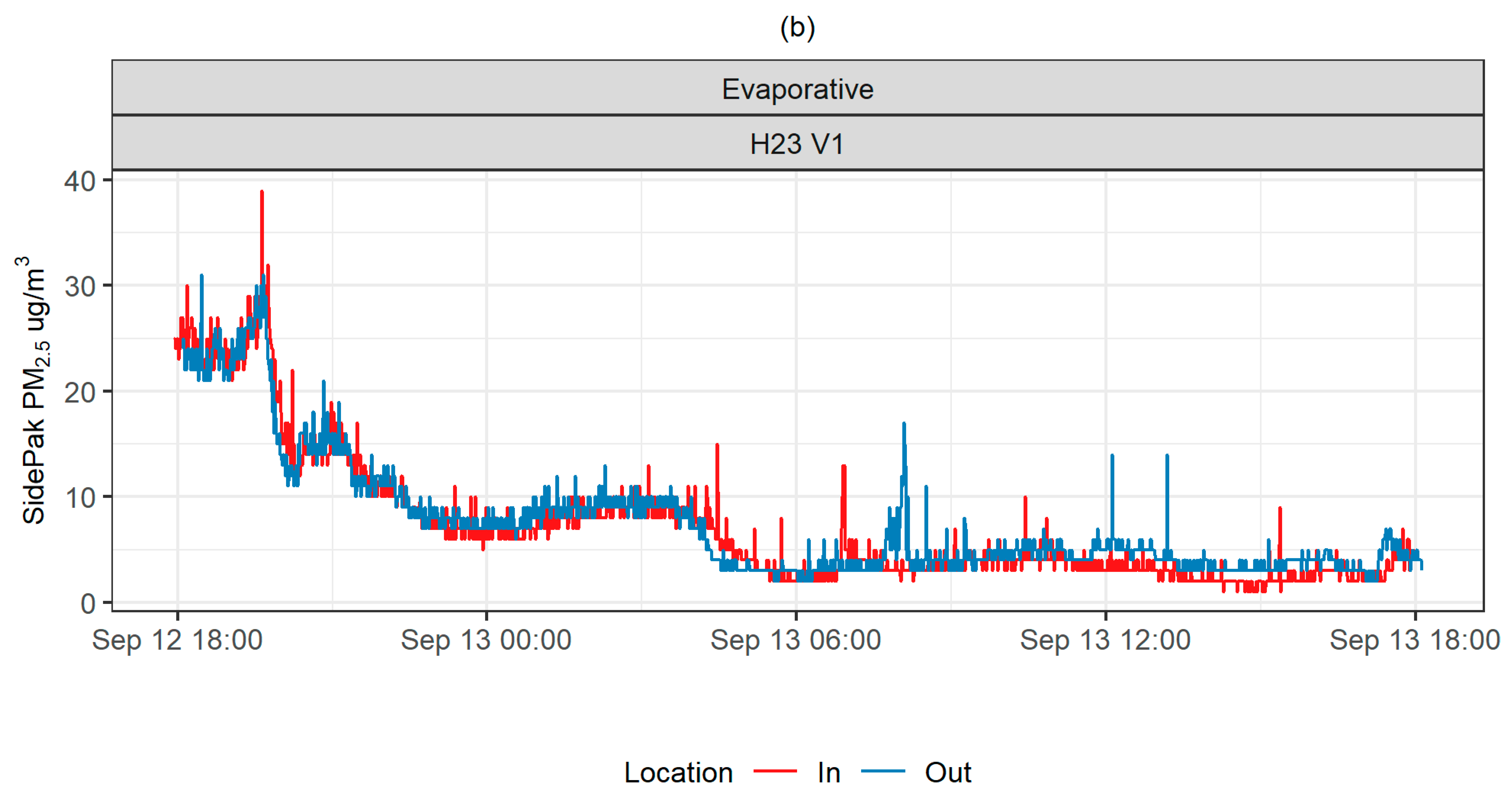
Figure 4 shows minute-by-minute SidePak PM2.5 concentrations for both indoor and outdoor locations for two example visits that occurred during the wildfire smoke event: Home 16 on 9–10 September 2022, and Home 23 on 12–13 September 2022. The time-series for all visits are shown in Figures S2–S4.

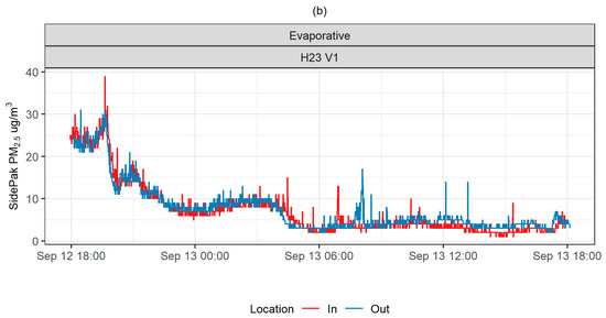
Figure 4.
Indoor and outdoor SidePak PM2.5 concentrations for (a) Home 16 on 9–10 September 2022 (Visit 2) and (b) Home 23 on 12–13 September 2022 (Visit 1).
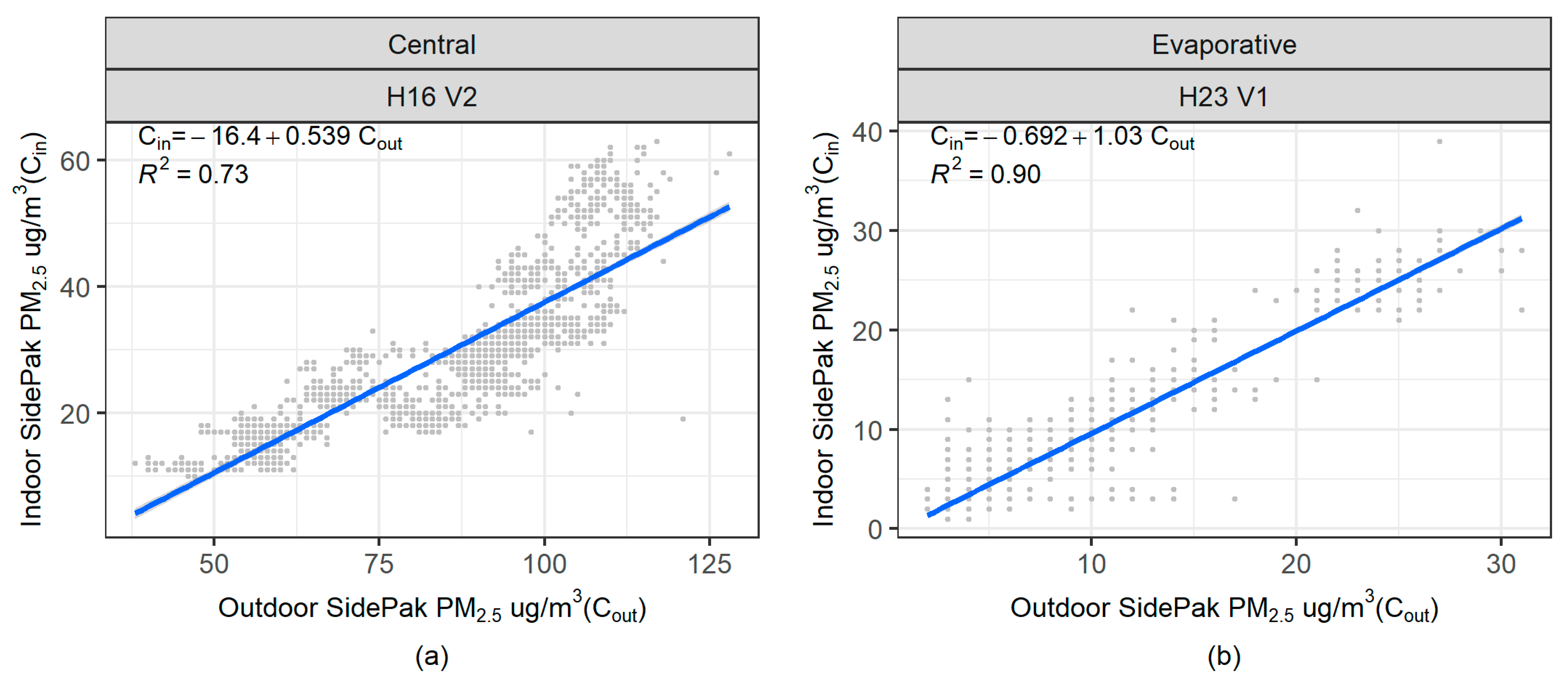
Figure 5 shows the correlation between the indoor and outdoor SidePak correlations for the two example visits. The coefficient estimates for Cs and Fin and the coefficient of determination (R2) measure of the goodness of fit of the model are also displayed. We have used R2 to quantify correlation because it explains the percent of variation in the indoor concentrations that is explained by the outdoor concentrations using the model form.
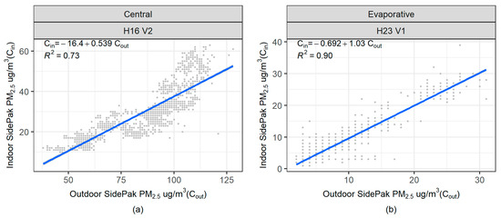
Figure 5.
Correlation of indoor and outdoor SidePak PM2.5 concentrations for two visits (a) Home 16 on 9–10 September 2022 (Visit 2) and (b) Home 23 on 12–13 September 2022 (Visit 1) with the Equation (1) coefficients, R2 goodness of fit, and model fit (displayed in blue).
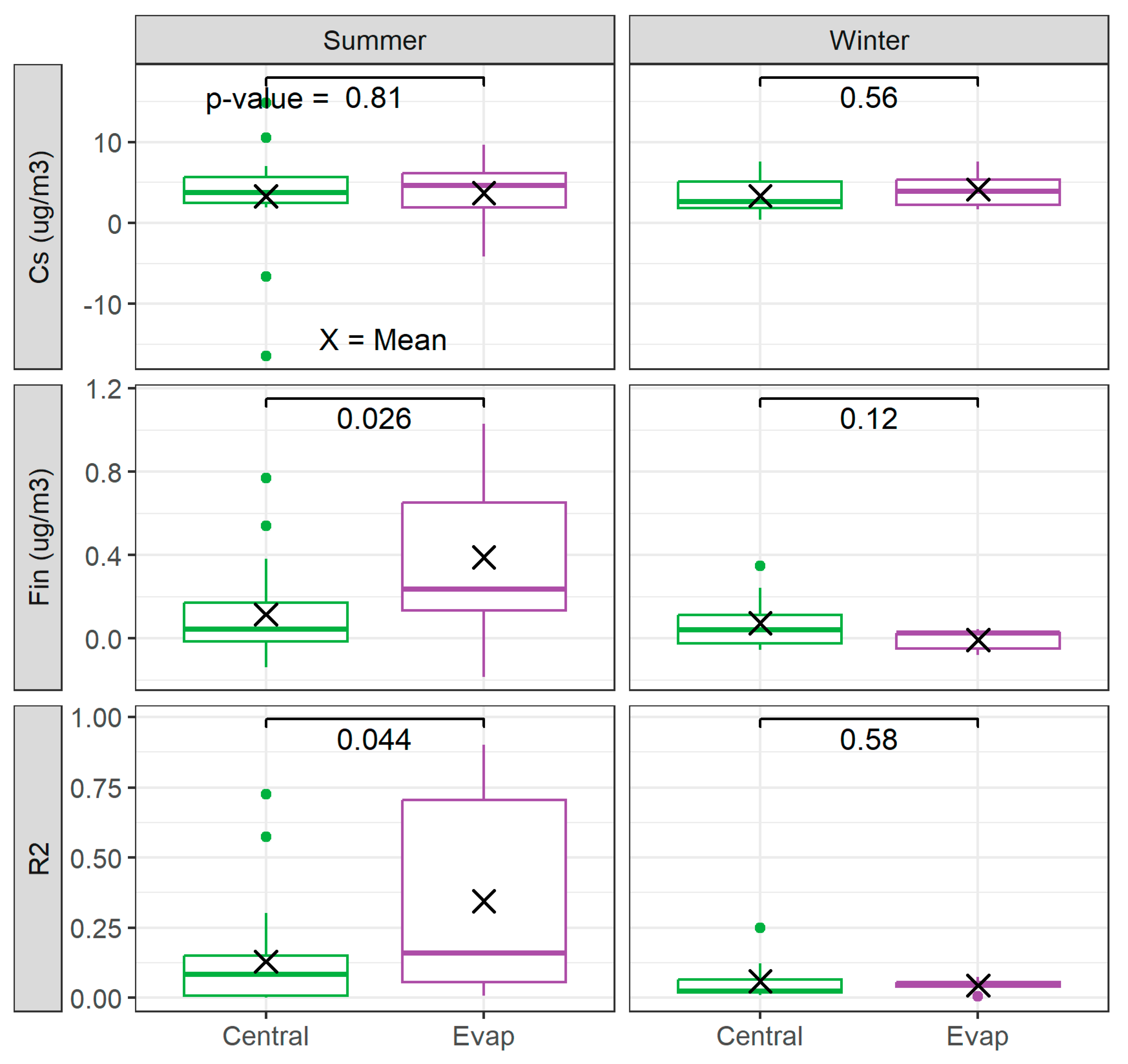
Figures S10–S12 show the correlation of indoor and outdoor minute-by-minute SidePak PM2.5 concentrations for each visit, along with the linear fit of Equation (1). Tables S9 and S10 contain the Cs, Fin, and R2 estimated for each home visit. Figure 6 summarizes the Cs, Fin, and R2 for each visit by air conditioning type and by season. We also calculated the mean Cs, Fin, and R2 value by air conditioning type (AC and EC) and season (summer and winter) using a simple average by treating each visit equally using Equations (S1)–(S3). The mean Cs, Fin, and R2 are also plotted in Figure 6, as are the p-values from a t-test evaluating differences in the mean Cs, Fin, and R2 data by type of air conditioner.
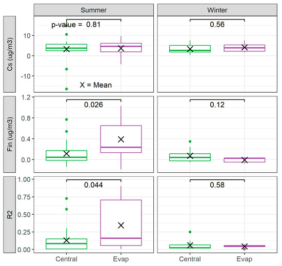
Figure 6.
Box plots of the Cs, Fin, and R2 estimated for each home visit organized by air conditioner type and season. The X symbols represent the mean value, and horizontal black lines and numbers are the p-values comparing the averages from two-sample t-tests.
The average Cs (the estimated contribution from indoor sources) ranges between 3.3 and 4.1 µg/m3 in the summer and winter (Table S11), and no significant differences are detected between the AC and EC visits. Although we asked participants to minimize indoor sources of air pollution in the homes, such as from cooking or candles, we still expect sources of indoor PM2.5, such as re-suspended dust from movement and air flow within the home [43]. We estimated negative Cs for just four of the fifty visits, all occurring during the wildfire smoke event (Tables S9 and S10 and Figure S14). In the winter, there is no discernable trend of Cs with outdoor PM2.5 concentrations (Figure S14). We believe that the Cs should be independent of the outdoor PM2.5 concentrations, and the negative Cs estimates in the summer are limitations of our correlation method to estimate indoor and outdoor contributions to the indoor PM2.5 concentrations.
In the summer, the average Fin for AC visits is 0.12 and more than two times higher (0.39) for visits in EC homes, and the difference is statistically significant (p-value =0.026). However, if we remove the seven wildfire smoke days, the difference is no longer statistically significant (Figure S13). The goodness of fit R2 is also higher for the EC visits than the AC visits.
In the winter, Fin is lower for both types of homes (0.07 for AC, and −0.01 for EC), but the difference is not statistically significant between AC and EC visits. The R2 for the winter visits is quite low for both types of air conditioners (0.06 for AC, and 0.04 for EC).
Fin varies considerably for the same homes between summer and winter visits. In addition, the infiltration factors from repeat measurements from the same home and same season also vary substantially, especially for AC visits in the summer (Figure S15). This suggests that ambient conditions influence Fin as much as, or more than, the properties of the home. In Figure S16, we plotted the Fin for each visit chronologically within season and home type. In general, the largest Fin occurred during the 8–12 September 2022 wildfire event for both AC and EC homes.
We evaluated if Fin in the summer was related to outdoor temperature, assuming that EC usage could increase with outdoor temperatures, which could increase the infiltration of outdoor particles. However, no clear trend is evident. If anything, Fin appeared to decrease with temperature for summer visits in homes with evaporative coolers (Figure S17). The lack of a clear trend in Fin with respect to temperature may be, in part, because we selected hot days for summer visits where the residents needed to use their AC or EC (Tables S5 and S7).
In the summer, Fin tends to increase with outdoor PM2.5 concentrations, which is consistent with the wildfire event observations. However, there is no trend in Fin with respect to outdoor PM2.5 concentrations during our winter observations (Figure S18).
3.4. Infiltration Factor Using Method 2
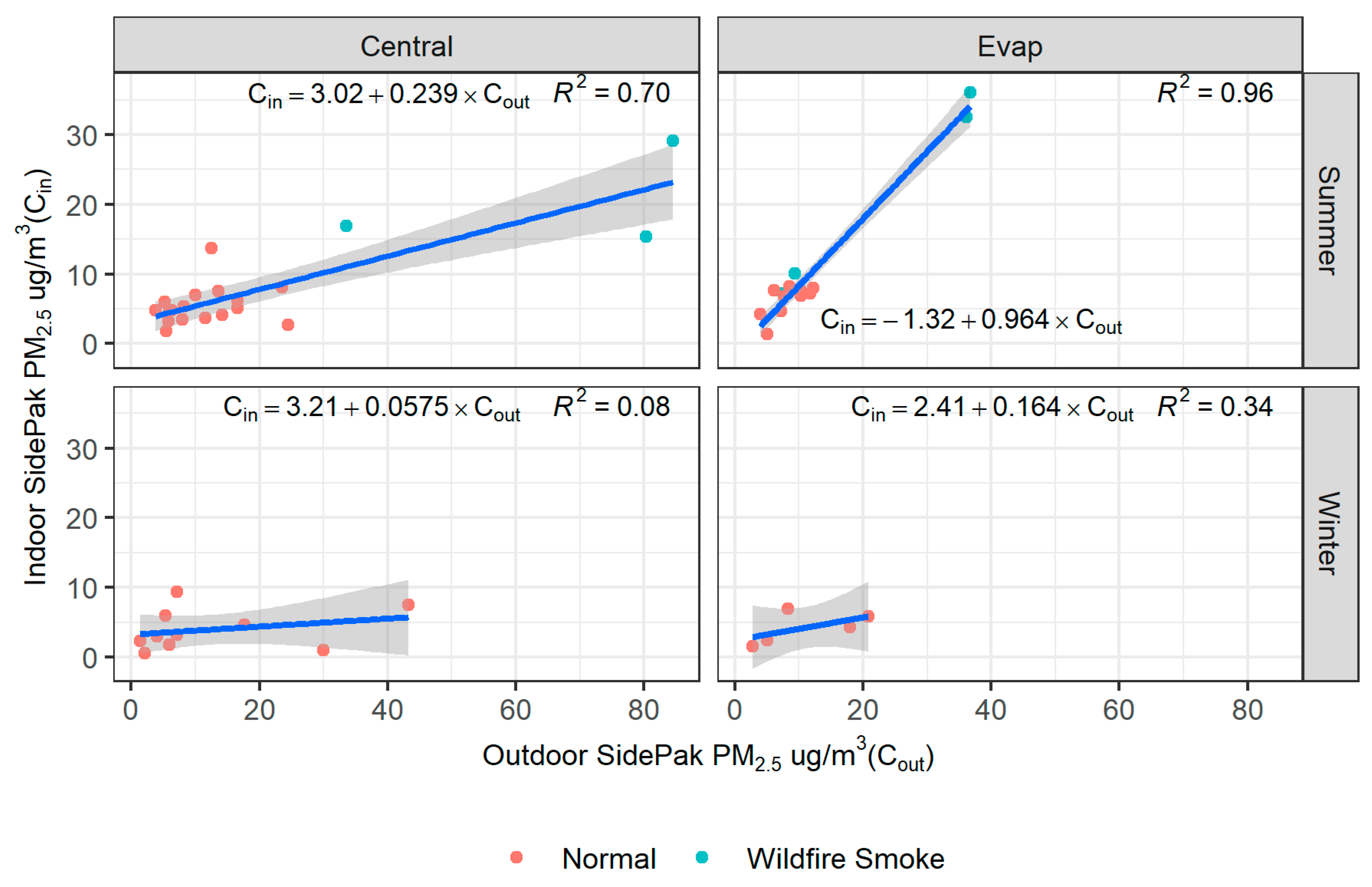
Figure 7 shows the average SidePak PM2.5 concentration data for each visit, with separate panels for air conditioner type (AC and EC) and season (summer and winter). The estimates of the infiltration factor (Fin) from Method 2 are displayed in Figure 7 with the fits of Equation (2) to each group of data. We observe a positive correlation in the indoor and outdoor PM2.5 concentrations across both types of homes and seasons. The slope, Fin, is consistently larger for the visits during the summer compared to winter, and for EC visits compared to AC visits. Additionally, the Fin estimated for EC visits (0.96) is more than four times the Fin for homes with AC (0.24). The difference in Fin between AC and EC visits in summer is highly significant (Table S13). In the winter, Fin is slightly positive, but is not significantly different than zero for either EC or AC visits (Table S12).
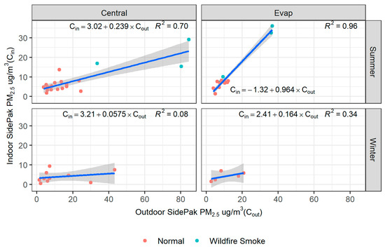
Figure 7.
Correlation of the average indoor and outdoor SidePak PM2.5 concentrations by season and air conditioner type. The Equation (2) coefficients, R2 goodness of fit, and model fit (displayed in blue). The grey shadow shows the observations that are within the standard error of the model prediction [42].
The estimates of linear regression coefficients (Cs and Fin) using Equation (2) are highly influenced by the home visits with large outdoor PM2.5 concentrations measured during the 8–12 September 2022 wildfire smoke event. When these seven days are removed, Fin is much smaller for both the visits in homes with AC and EC (Figure S19). The Fin for AC visits is moderately positive but is no longer significantly different than zero (Table S12). The Fin for EC visits is still strongly positive (0.54) and significantly different than zero. However, Fin is no longer significantly different (p-value = 0.14) between AC and EC visits (Table S15).
3.5. Comparison of Infiltration Factors between Method 1 and Method 2
In Table 2, we compared the mean Fin estimated using Method 1 with the Fin estimated using Method 2 for the AC and EC visits conducted in the summer.
Table 2.
Infiltration factor (Fin) estimated from Method 1 and Method 2 for summer visits.
The Fin obtained using Method 2 is substantially larger for both types of homes. Despite the differences, both methods estimate that Fin is larger in EC homes. We believe there are two factors that lead to higher Fin estimates using Method 2.
- (1)
- As noted in Section 3.3, the Fin from Method 1 increases with outdoor PM2.5 concentrations. However, the wildfire smoke visits only account for seven of the thirty home visits conducted in the summer. Because we calculated the mean Fin treating each visit equally (Equation (S2)), the average Fin from Method 1 is substantially lower than the individual days with wildfire smoke.
- (2)
- The infiltration factors estimated for the summer from Method 2 are highly influenced by the seven visits that occurred on the wildfire smoke days. As shown in Figure 7, the wildfire smoke visits are outside the cloud of visits on other days, making the wildfire visits very influential on the estimate of Fin. The estimate of Fin including the days with wildfire smoke was 0.96 for EC visits, but only 0.57 when removing the wildfire smoke days.
We believe the estimates from Method 2 are most appropriate for estimating the Fin for days with wildfire smoke and Method 1 is appropriate for estimating the Fin for an average summer day. The individual Fin estimated from Method 1 from the wildfire smoke days ranged from 0.27 to 0.54 for AC visits (three visits), and 0.81 to 1.03 for EC visits (four visits) (Tables S9 and S10). The individual Fin from the wildfire smoke days correspond better to the Fin estimated from Method 2, particularly for EC homes. In winter, the two methods yielded more comparable estimates for Fin (Table S16).
The infiltration factors estimated from our study for AC homes in wildfire events are near the bottom range reported from previous indoor air quality studies in the US, which range between 0.2 and 0.8 [41,44,45]. However, individual study homes (presumably AC) have been observed across a much broader range between 0.01 and 0.87 during wildfire smoke events [46]. The Fin estimates for EC homes on average summer days fall within the range of the literature values. However, the Fin from EC homes measured during the wildfire smoke event in our study were close to 1, which extends beyond the range of previously reported values.
4. Discussion
Evaporative cooling offers a low-energy alternative to AC, and wider acceptance and use of ECs in arid and semi-arid regions globally may partially offset projected increases in energy use associated with residential space cooling. To be considered as a sustainable alternative to AC, however, ECs should not put home occupants at higher risk of exposure to outdoor air pollution that infiltrates the home through the cooler. For average summer days in our study, EC homes provided a modest amount of protection (Fin of 0.39), but AC homes provided a greater amount of protection (Fin of 0.12). No difference in infiltration factor by air conditioning type was observed during the winter when air conditioning is not in use. Thus, we believe the differences we observe in summer can be attributed to the use of air conditioning and not to other factors related to the homes.
Our findings agree with the existing literature regarding infiltration of PM2.5 into EC homes. The I/O ratio (0.83) for EC homes in our study falls within the range of 0.63–1.04 reported in prior studies [23,28]. One strength of our study was the addition of a comparison group of AC homes, which previous studies lacked. AC homes in our study offered significantly greater protection (I/O ratio = 0.55; p-value = 0.006) from infiltration of outdoor air pollution, and this was most noticeable during a wildfire smoke event that occurred during the study period. Our analysis suggests that EC homes provide little to no protection from outdoor PM2.5 during wildfire events in the summer (Fin of 0.96), when the PM2.5 concentrations are highest, and protection is most desired. Similar homes in Utah County equipped with AC benefited from a substantial amount of protection from outdoor PM2.5 pollution during the same wildfire event (Fin of 0.23).
Higher infiltration factors have been observed during wildfire smoke days in nursing homes compared to normal days (0.59 vs. 0.43) [44], whereas a large study using crowdsourced home monitor data in California estimated lower infiltration of outdoor PM2.5 during wildfire events, which is attributed to residents changing their behavior in response to poor air quality, such as closing windows and using air purifiers on poor air quality days [45].
We believe that changes in particle size, morphology, and composition is a driving factor for the larger infiltration of particles during summer, including wildfire smoke events. During winter inversions, the PM2.5 composition in Utah County is dominated by ammonium nitrate [47], which evaporates indoors at warm temperatures and low humidity [48]. Other studies have also demonstrated lower Fin values during winter compared to summer [49]. On the other hand, carbonaceous wood smoke particles have been shown to effectively infiltrate and remain airborne in particle phase inside homes [46,50] and other buildings [44].
By conducting 24 h samples, the results from each home in our study were limited to the types of conditions measured. Thus, our study results were highly influenced by the seven home visits we conducted during one single wildfire smoke event. For future studies, we recommend using many continuous monitors, so that that each home is sampled over the same conditions, especially during any high PM2.5 pollution events. We also recommend conducting sampling over longer periods of time inside homes without restrictions on aerosol-producing activities, as were in place in this study. This will allow for evaluation of how ECs can mitigate indoor air pollution sources through their large ACH rates, which we intentionally avoided in our study. This study was limited to single-family homes in one county in Utah. Thus, our findings may not be generalizable to multi-unit dwellings. In addition, housing envelopes vary widely across regions based on cost and available building materials, which may influence PM2.5 infiltration differently than homes in our study. Thus, our findings may not be generalizable to homes in other regions.
In our study, our instruments only measured PM2.5 particles. We acknowledge that we are missing the potential effectiveness of ECs in removing PM10 particles. PM10 is an important measure of dust that can occur in high levels during dust storms in Utah and other arid regions that can also utilize ECs, and should be considered in future studies [47,51].
Several of the study participants living in homes with ECs reported that they limit the use of their ECs during days with poor air quality. Our study confirms that this can be an effective strategy to improve indoor air quality, but may not be possible or desirable for the residents if the EC is their only way to effectively cool their home.
Although not a randomized study, the average age of EC homes (61 years) was much older than for AC homes (35 years). Additionally, the residents who participated in the study who lived in EC homes were more likely to rent their home than the participants who lived in AC homes (Table 1). Thus, our study suggests that the use of ECs in older homes may contribute to disparities in air pollution exposure by social and economic factors among residents living in Utah County. Because of their low cost and energy-efficiency, we recommend additional research to evaluate EC interventions that can reduce the infiltration of outdoor PM2.5.
5. Conclusions
In arid and semi-arid regions, evaporative cooling has strong potential to help offset energy use associated with the rapidly growing demand for residential air conditioning. One barrier to their success as a sustainable alternative to AC, however, is the possibility of infiltration of outdoor PM2.5 and its associated health effects. Prior research on ECs primarily focuses on system efficiencies such as air flow rate and pressure drop, water consumption, heat and mass transfer, and degradation of pad materials [52,53,54]. Our findings suggest a need for studies focused on EC design specifically to decrease infiltration of particle-phase pollutants. Improved EC cooling pads, for instance, may have utility in serving a dual purpose of providing an efficient wetting medium while also serving as an effective filter for fine particulates. Optimal pad configurations for efficiency and particle removal, tailored to local air pollution conditions, may then be recommended to EC users.
Supplementary Materials
The following supporting information can be downloaded at: https://www.mdpi.com/article/10.3390/su16010177/s1, S.1 Classification of Wildfire Smoke Events, S.2. Removal of Incomplete Data, S.3 Inspection of minute-by-minute Sidepak PM2.5 Data, S.4 Comparison of PM2.5 Measurements from the SidePak to the Utah Division of Air Quality (UDAQ) Monitors, S.5 Indoor/Outdoor PM2.5 Ratios S.6 Temperature and Relative Humidity Data, S.7 Infiltration Factor Estimates using Method 1, S.8 Summary Statistics from Method 1, S.9 Infiltration Factor Estimates using Method 2. S.10 Comparison of Infiltration Factor Estimates using Method 1 and Method 2. S.11 References [55,56,57,58].
Author Contributions
Conceptualization, D.B.S. and J.D.J.; methodology, D.B.S., H.J., R.P.H., T.C.P., S.E.W., T.R.C. and J.D.J.; validation, D.B.S., H.J. and R.P.H.; formal analysis, D.B.S., H.J. and R.P.H.; investigation, D.B.S., H.J., R.P.H., T.C.P., S.E.W., T.R.C. and J.D.J.; resources, D.B.S. and J.D.J.; data curation, D.B.S., H.J. and R.P.H.; writing—original draft preparation, D.B.S., H.J., R.P.H., T.C.P., T.R.C. and J.D.J.; writing—review and editing, D.B.S., H.J., R.P.H., T.C.P., S.E.W., T.R.C. and J.D.J.; visualization, D.B.S., H.J., R.P.H., T.C.P., T.R.C. and J.D.J.; supervision, D.B.S. and J.D.J.; project administration, D.B.S. and J.D.J.; funding acquisition, D.B.S., S.E.W. and J.D.J. All authors have read and agreed to the published version of the manuscript.
Funding
This work was supported in part by a College Undergraduate Research Award from Brigham Young University’s College of Life Sciences and an Experiential Learning Grant from the Ira A. Fulton College of Engineering.
Institutional Review Board Statement
The Institutional Review Board at Brigham Young University (BYU) determined that the unit of study was the home, not the occupant(s), and thus did not require the human subjects’ research approval.
Informed Consent Statement
Informed consent was obtained from all subjects involved in the study.
Data Availability Statement
The data and analysis scripts are publically available at https://github.com/darrell-sonntag/EvapCoolerUtahCounty, accessed 21 December 2023. The information from the participant survey is also made available, except for any information which could be used to identify the homes in the study (address and home area).
Acknowledgments
We acknowledge the full team of BYU students who worked on this project, including: Paula Chanthakhoun, Alisandra Olivares, Seth Van Roosendaal, Julianna Stock, Jaxson Tadje, Braedon Tarone, Joseph West, and Dallin Widowski. We are especially grateful to the participants who allowed us access to their homes to conduct this research.
Conflicts of Interest
The authors declare no conflicts of interest.
References
- Davis, L.; Gertler, P.; Jarvis, S.; Wolfram, C. Air conditioning and global inequality. Glob. Environ. Chang. 2021, 69, 102299. [Google Scholar] [CrossRef]
- Akpinar-Ferrand, E.; Singh, A. Modeling increased demand of energy for air conditioners and consequent CO2 emissions to minimize health risks due to climate change in India. Environ. Sci. Policy 2010, 13, 702–712. [Google Scholar] [CrossRef]
- Vakiloroaya, V.; Samali, B.; Fakhar, A.; Pishghadam, K. A review of different strategies for HVAC energy saving. Energy Convers. Manag. 2014, 77, 738–754. [Google Scholar] [CrossRef]
- El-Dessouky, H.; Ettouney, H.; Al-Zeefari, A. Performance analysis of two-stage evaporative coolers. Chem. Eng. J. 2004, 102, 255–266. [Google Scholar] [CrossRef]
- Saidur, R.; Masjuki, H.H.; Jamaluddin, M. An application of energy and exergy analysis in residential sector of Malaysia. Energy Policy 2007, 35, 1050–1063. [Google Scholar] [CrossRef]
- Swan, L.G.; Ugursal, V.I. Modeling of end-use energy consumption in the residential sector: A review of modeling techniques. Renew. Sustain. Energy Rev. 2009, 13, 1819–1835. [Google Scholar] [CrossRef]
- Isaac, M.; Van Vuuren, D.P. Modeling global residential sector energy demand for heating and air conditioning in the context of climate change. Energy Policy 2009, 37, 507–521. [Google Scholar] [CrossRef]
- Davis, L.W.; Gertler, P.J. Contribution of air conditioning adoption to future energy use under global warming. Proc. Natl. Acad. Sci. USA 2015, 112, 5962–5967. [Google Scholar] [CrossRef]
- Watt, J.R.; Brown, W.K. Evaporative Air Conditioning Handbook, 3rd ed.; Fairmont Press: Upper Saddle River, NJ, USA, 1997. [Google Scholar]
- Bom, G.J. Evaporative Air-Conditioning: Applications for Environmentally Friendly Cooling; World Bank Publications: Washington, DC, USA, 1999; Volume 23. [Google Scholar]
- Yang, Y.; Cui, G.; Lan, C.Q. Developments in evaporative cooling and enhanced evaporative cooling—A review. Renew. Sustain. Energy Rev. 2019, 113, 109230. [Google Scholar] [CrossRef]
- McNeil, M.A.; Letschert, V.E. Future Air Conditioning Energy Consumption in Developing Countries and What Can Be Done About It: The Potential of Efficiency in the Residential Sector. 2008. Available online: https://escholarship.org/content/qt64f9r6wr/qt64f9r6wr.pdf (accessed on 21 December 2023).
- Nabokov, P.; Easton, R. Native American Architecture; Oxford University Press: Oxford, UK, 1990. [Google Scholar]
- Cunningham, B. The box that broke the barrier: The swamp cooler comes to Southern Arizona. J. Ariz. Hist. 1985, 26, 163–174. [Google Scholar]
- Speid, M.J.B. Our Last Years in India; Smith, Elder and Co.: London, UK, 1862. [Google Scholar]
- Bahadori, M.N. Passive Cooling Systems in Iranian Architecture; Scientific American: New York, NY, USA, 2018; Volume 238, pp. 144–155. [Google Scholar]
- Jomehzadeh, F.; Nejat, P.; Calautit, J.K.; Yusof, M.B.M.; Zaki, S.A.; Hughes, B.R.; Yazid, M.N.A.W.M. A review on windcatcher for passive cooling and natural ventilation in buildings, Part 1: Indoor air quality and thermal comfort assessment. Renew. Sustain. Energy Rev. 2017, 70, 736–756. [Google Scholar] [CrossRef]
- Malli, A.; Seyf, H.R.; Layeghi, M.; Sharifian, S.; Behravesh, H. Investigating the performance of cellulosic evaporative cooling pads. Energy Convers. Manag. 2011, 52, 2598–2603. [Google Scholar] [CrossRef]
- Nada, S.; Fouda, A.; Mahmoud, M.; Elattar, H. Experimental investigation of energy and exergy performance of a direct evaporative cooler using a new pad type. Energy Build. 2019, 203, 109449. [Google Scholar] [CrossRef]
- Fouda, A.; Melikyan, Z. A simplified model for analysis of heat and mass transfer in a direct evaporative cooler. Appl. Therm. Eng. 2011, 31, 932–936. [Google Scholar] [CrossRef]
- Chiesa, G.; Pearlmutter, D. Ventilative Cooling in Combination with Other Natural Cooling Solutions: Direct Evaporative Cooling—DEC. In Innovations in Ventilative Cooling; Springer: Berlin/Heidelberg, Germany, 2021; pp. 167–190. [Google Scholar]
- Macher, J.M.; Girman, J.R. Multiplication of microorganisms in an evaporative air cooler and possible indoor air contamination. Environ. Int. 1990, 16, 203–211. [Google Scholar] [CrossRef]
- Li, W.-W.; Paschold, H.; Morales, H.; Chianelli, J. Correlations between short-term indoor and outdoor PM concentrations at residences with evaporative coolers. Atmos. Environ. 2003, 37, 2691–2703. [Google Scholar] [CrossRef]
- Yamamoto, N.; Shendell, D.; Winer, A.; Zhang, J. Residential air exchange rates in three major US metropolitan areas: Results from the Relationship Among Indoor, Outdoor, and Personal Air Study 1999–2001. Indoor Air 2010, 20, 85–90. [Google Scholar] [CrossRef]
- Quackenboss, J.J.; Lebowitz, M.D.; Crutchfield, C.D. Indoor-outdoor relationships for particulate matter: Exposure classifications and health effects. Environ. Int. 1989, 15, 353–360. [Google Scholar] [CrossRef]
- Pope, C.A., III; Lefler, J.S.; Ezzati, M.; Higbee, J.D.; Marshall, J.D.; Kim, S.-Y.; Bechle, M.; Gilliat, K.S.; Vernon, S.E.; Robinson, A.L. Mortality risk and fine particulate air pollution in a large, representative cohort of US adults. Environ. Health Perspect. 2019, 127, 077007. [Google Scholar] [CrossRef]
- Pope, C.A., III; Dockery, D.W. Health effects of fine particulate air pollution: Lines that connect. J. Air Waste Manag. Assoc. 2006, 56, 709–742. [Google Scholar] [CrossRef]
- Paschold, H.; Li, W.-W.; Morales, H.; Walton, J. Laboratory study of the impact of evaporative coolers on indoor PM concentrations. Atmos. Environ. 2003, 37, 1075–1086. [Google Scholar] [CrossRef]
- Weber, K.T.; Yadav, R. Spatiotemporal trends in wildfires across the Western United States (1950–2019). Remote Sens. 2020, 12, 2959. [Google Scholar] [CrossRef]
- Dennison, P.E.; Brewer, S.C.; Arnold, J.D.; Moritz, M.A. Large wildfire trends in the western United States, 1984–2011. Geophys. Res. Lett. 2014, 41, 2928–2933. [Google Scholar] [CrossRef]
- McClure, C.D.; Jaffe, D.A. US particulate matter air quality improves except in wildfire-prone areas. Proc. Natl. Acad. Sci. USA 2018, 115, 7901–7906. [Google Scholar] [CrossRef] [PubMed]
- US Forest Service and US EPA, Fire and Smoke Map 3.1, Collaborative Effort between the U.S. Forest Service (USFS)-Led Interagency Wildland Fire Air Quality Response Program and the U.S. Environmental Protection Agency (EPA). Available online: https://fire.airnow.gov/ (accessed on 13 November 2023).
- ISO 12103-1:2016; Road Vehicles – Test Contaminants for Filter Evaluation – Part 1: Arizona Test Dust. International Organization for Standardization: Geneva, Switzerland, 2016.
- Sioutas, C.; Kim, S.; Chang, M.; Terrell, L.L.; Gong, H., Jr. Field evaluation of a modified DataRAM MIE scattering monitor for real-time PM2. 5 mass concentration measurements. Atmos. Environ. 2000, 34, 4829–4838. [Google Scholar] [CrossRef]
- Wang, Y.; Li, J.; Jing, H.; Zhang, Q.; Jiang, J.; Biswas, P. Laboratory evaluation and calibration of three low-cost particle sensors for particulate matter measurement. Aerosol Sci. Technol. 2015, 49, 1063–1077. [Google Scholar] [CrossRef]
- Yu, C.H.; Patton, A.P.; Zhang, A.; Fan, Z.-H.; Weisel, C.P.; Lioy, P.J. Evaluation of diesel exhaust continuous monitors in controlled environmental conditions. J. Occup. Environ. Hyg. 2015, 12, 577–587. [Google Scholar] [CrossRef]
- Jaffe, D.A.; Thompson, K.; Finley, B.; Nelson, M.; Ouimette, J.; Andrews, E. An evaluation of the US EPA’s correction equation for PurpleAir sensor data in smoke, dust, and wintertime urban pollution events. Atmos. Meas. Tech. 2023, 16, 1311–1322. [Google Scholar] [CrossRef]
- Wang, Z.; Wang, D.; Peng, Z.-R.; Cai, M.; Fu, Q.; Wang, D. Performance assessment of a portable nephelometer for outdoor particle mass measurement. Environ. Sci. Process. Impacts 2018, 20, 370–383. [Google Scholar] [CrossRef]
- Ramachandran, G.; Adgate, J.L.; Pratt, G.C.; Sexton, K. Characterizing indoor and outdoor 15 minute average PM 2.5 concentrations in urban neighborhoods. Aerosol Sci. Technol. 2003, 37, 33–45. [Google Scholar] [CrossRef]
- Soneja, S.; Chen, C.; Tielsch, J.M.; Katz, J.; Zeger, S.L.; Checkley, W.; Curriero, F.C.; Breysse, P.N. Humidity and gravimetric equivalency adjustments for nephelometer-based particulate matter measurements of emissions from solid biomass fuel use in cookstoves. Int. J. Environ. Res. Public Health 2014, 11, 6400–6416. [Google Scholar] [CrossRef] [PubMed]
- Chen, C.; Zhao, B. Review of relationship between indoor and outdoor particles: I/O ratio, infiltration factor and penetration factor. Atmos. Environ. 2011, 45, 275–288. [Google Scholar] [CrossRef]
- Wickham, H. ggplot2: Elegant Graphics for Data Analysis; Springer: New York, NY, USA, 2016; Available online: https://ggplot2.tidyverse.org/ (accessed on 2 November 2023).
- Goldstein, A.H.; Nazaroff, W.W.; Weschler, C.J.; Williams, J. How do indoor environments affect air pollution exposure? Environ. Sci. Technol. 2020, 55, 100–108. [Google Scholar] [CrossRef] [PubMed]
- Montrose, L.; Walker, E.S.; Toevs, S.; Noonan, C.W. Outdoor and indoor fine particulate matter at skilled nursing facilities in the western United States during wildfire and non-wildfire seasons. Indoor Air 2022, 32, e13060. [Google Scholar] [CrossRef] [PubMed]
- Liang, Y.; Sengupta, D.; Campmier, M.J.; Lunderberg, D.M.; Apte, J.S.; Goldstein, A.H. Wildfire smoke impacts on indoor air quality assessed using crowdsourced data in California. Proc. Natl. Acad. Sci. USA 2021, 118, e2106478118. [Google Scholar] [CrossRef] [PubMed]
- May, N.W.; Dixon, C.; Jaffe, D.A. Impact of wildfire smoke events on indoor air quality and evaluation of a low-cost filtration method. Aerosol Air Qual. Res. 2021, 21, 210046. [Google Scholar] [CrossRef]
- Flowerday, C.E.; Thalman, R.; Hansen, J.C. Twenty-Year Review of Outdoor Air Quality in Utah, USA. Atmosphere 2023, 14, 1496. [Google Scholar] [CrossRef]
- Lunden, M.M.; Revzan, K.L.; Fischer, M.L.; Thatcher, T.L.; Littlejohn, D.; Hering, S.V.; Brown, N.J. The transformation of outdoor ammonium nitrate aerosols in the indoor environment. Atmos. Environ. 2003, 37, 5633–5644. [Google Scholar] [CrossRef]
- Barn, P.; Larson, T.; Noullett, M.; Kennedy, S.; Copes, R.; Brauer, M. Infiltration of forest fire and residential wood smoke: An evaluation of air cleaner effectiveness. J. Expo. Sci. Environ. Epidemiol. 2008, 18, 503–511. [Google Scholar] [CrossRef]
- Sparks, T.L.; Wagner, J. Composition of particulate matter during a wildfire smoke episode in an urban area. Aerosol Sci. Technol. 2021, 55, 734–747. [Google Scholar] [CrossRef]
- Goodman, M.M.; Carling, G.T.; Fernandez, D.P.; Rey, K.A.; Hale, C.A.; Bickmore, B.R.; Nelson, S.T.; Munroe, J.S. Trace element chemistry of atmospheric deposition along the Wasatch Front (Utah, USA) reflects regional playa dust and local urban aerosols. Chem. Geol. 2019, 530, 119317. [Google Scholar] [CrossRef]
- Tejero-González, A.; Franco-Salas, A. Optimal operation of evaporative cooling pads: A review. Renew. Sustain. Energy Rev. 2021, 151, 111632. [Google Scholar] [CrossRef]
- Kapilan, N.; Isloor, A.M.; Karinka, S. A comprehensive review on evaporative cooling systems. Results Eng. 2023, 18, 101059. [Google Scholar] [CrossRef]
- Amer, O.; Boukhanouf, R.; Ibrahim, H.G. A review of evaporative cooling technologies. Int. J. Environ. Sci. Dev. 2015, 6, 111. [Google Scholar] [CrossRef]
- US EPA. Outdoor Air Quality Data; 2023. Available online: https://www.epa.gov/outdoor-air-quality-data/download-daily-data (accessed on 13 November 2023).
- US EPA. AirNow API; 2023. Available online: https://docs.airnowapi.org/ (accessed on 14 November 2023).
- UDAQ. Annual Monitoring Network Plan 2022; Utah Department of Environmental Quality, 2023. Available online: https://documents.deq.utah.gov/air-quality/planning/air-monitoring/DAQ-2022-007189.pdf (accessed on 19 July 2023).
- National Weather Service. NOWData-NOAA Online Weather Data. 2023. Available online: https://www.weather.gov/wrh/Climate?wfo=slc (accessed on 11 October 2023).
Disclaimer/Publisher’s Note: The statements, opinions and data contained in all publications are solely those of the individual author(s) and contributor(s) and not of MDPI and/or the editor(s). MDPI and/or the editor(s) disclaim responsibility for any injury to people or property resulting from any ideas, methods, instructions or products referred to in the content. |
© 2023 by the authors. Licensee MDPI, Basel, Switzerland. This article is an open access article distributed under the terms and conditions of the Creative Commons Attribution (CC BY) license (https://creativecommons.org/licenses/by/4.0/).