
Long-Term Forecasting of Air Pollution Particulate Matter (PM2.5) and Analysis of Influencing Factors


Abstract
:1. Introduction
- Comparing the performance of 10 mainstream models in long-term PM2.5 forecasting;
- Exploring the application of explainable AI technology in air-pollution-prediction systems;
- Analyzing environmental factors affecting PM2.5 levels from the perspective of individual factors and the interaction between factors.
2. Related Work
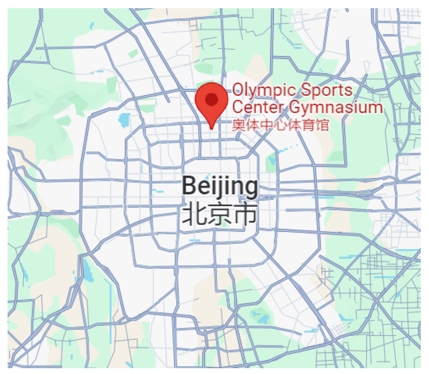
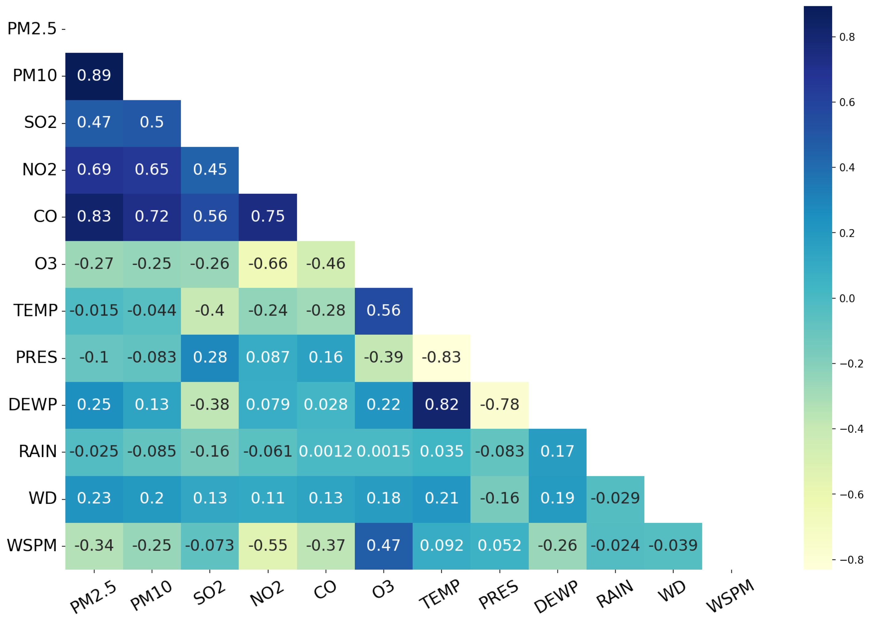
3. Data Description
4. Method
4.1. Data Processing and Influencing Factors’ Analysis Process
4.2. Forecasting Methods
4.2.1. Ensemble Learning
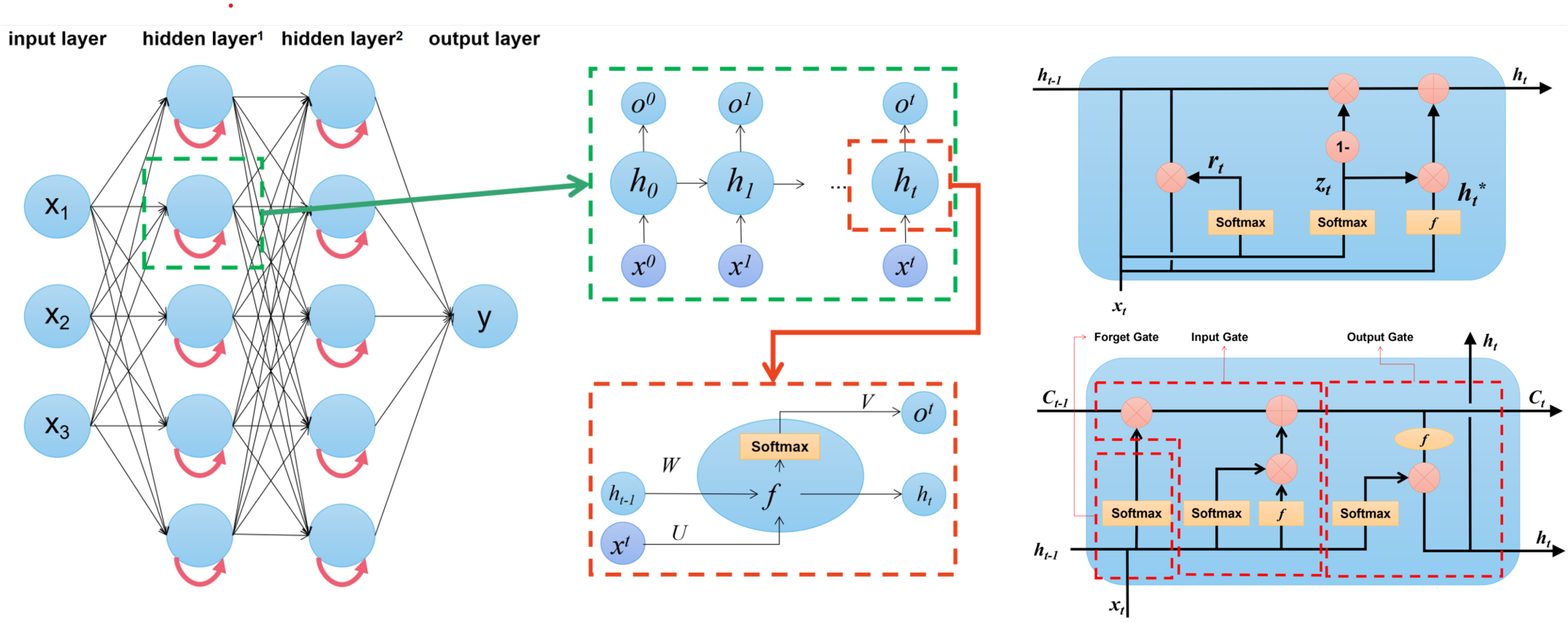
4.2.2. Multilayer Perceptron
4.2.3. RNN-Based Models
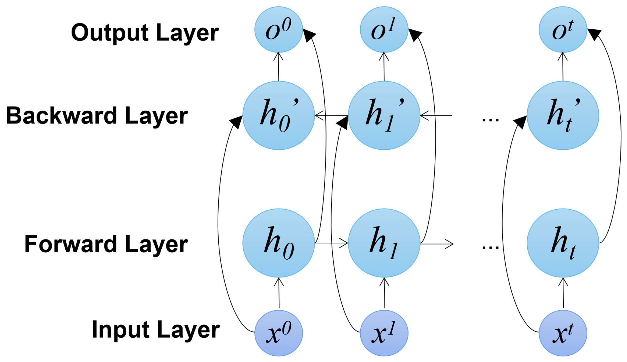
4.2.4. Bi-Directional-RNN-Based Models
4.3. Explainable AI
4.4. Objective Function
5. Results
5.1. Results of Forecasting Performance
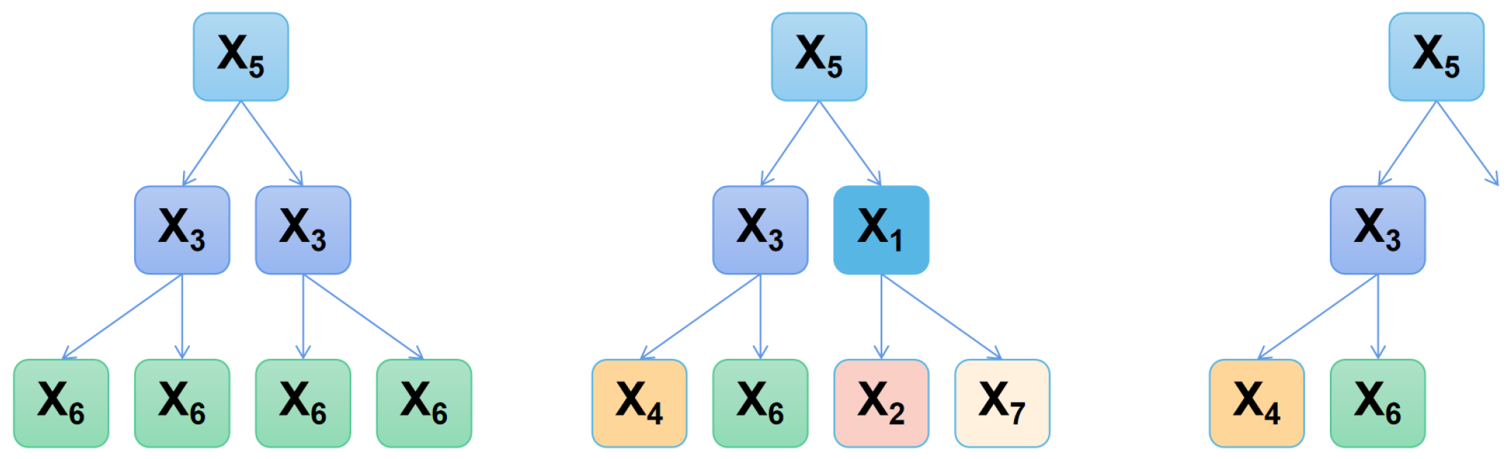
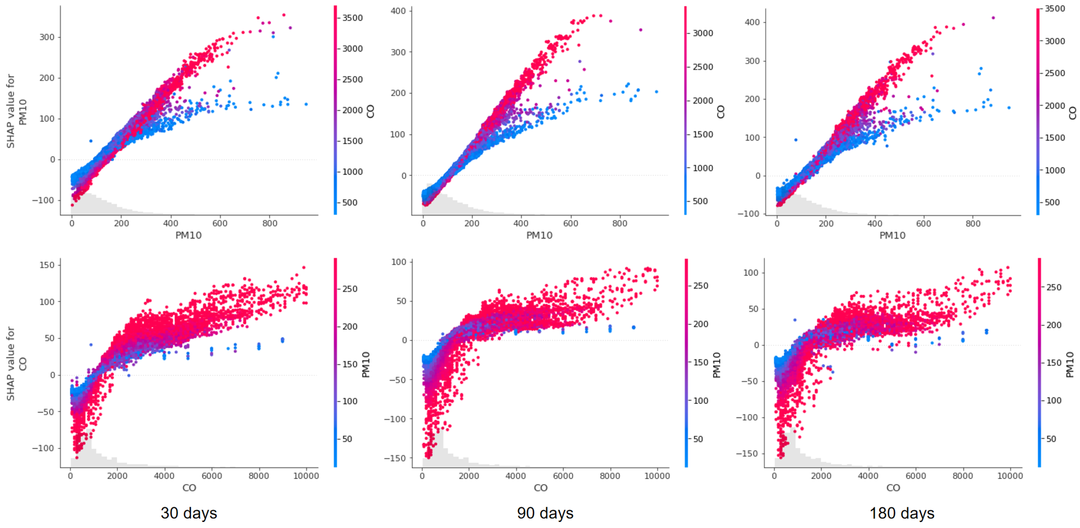
5.2. Analysis of Influencing Factors
5.2.1. Impact Analysis of Single Factor
5.2.2. Interaction Analysis of Factors
5.3. Findings from the Analysis
6. Discussion
- “I like playing the piano and playing basketball.”
- “I like playing basketball and playing the piano.”
7. Conclusions
Author Contributions
Funding
Data Availability Statement
Conflicts of Interest
References
- Maciejczyk, P.; Chen, L.C.; Thurston, G. The role of fossil fuel combustion metals in PM2.5 air pollution health associations. Atmosphere 2021, 12, 1086. [Google Scholar] [CrossRef]
- Meo, S.A.; Almutairi, F.J.; Abukhalaf, A.A. Effect of green space environment on air pollutants PM2.5, PM10, CO, O3, and incidence and mortality of SARS-CoV-2 in highly green and less-green countries. Int. J. Environ. Res. Public Health 2021, 18, 13151. [Google Scholar] [CrossRef]
- Fan, Z.; Zhan, Q.; Yang, C. How did distribution patterns of particulate matter air pollution (PM2.5 and PM10) change in China during the COVID-19 outbreak: A spatiotemporal investigation at Chinese city-level. Int. J. Environ. Res. Public Health 2020, 17, 6274. [Google Scholar] [CrossRef]
- Wang, Z.; Chen, L.; Ding, Z. An enhanced interval PM2.5 concentration forecasting model based on BEMD and MLPI with influencing factors. Atmos. Environ. 2020, 223, 117200. [Google Scholar] [CrossRef]
- Delp, W.W.; Singer, B.C. Wildfire smoke adjustment factors for low-cost and professional PM2.5 monitors with optical sensors. Sensors 2020, 20, 3683. [Google Scholar] [CrossRef]
- Luo, H.; Han, Y.; Lu, C. Characteristics of surface solar radiation under different air pollution conditions over Nanjing, China: Observation and simulation. Adv. Atmos. Sci. 2019, 36, 1047–1059. [Google Scholar] [CrossRef]
- Fan, H.; Zhao, C.; Yang, Y. Spatio-temporal variations of the PM2.5/PM10 ratios and its application to air pollution type classification in China. Front. Environ. Sci. 2021, 9, 692440. [Google Scholar] [CrossRef]
- Spandana, B.; Rao, S.S.; Upadhya, A.R. PM2.5/PM10 ratio characteristics over urban sites of India. Adv. Space Res. 2021, 67, 3134–3146. [Google Scholar] [CrossRef]
- Al-Janabi, S.; Alkaim, A.; Al-Janabi, E. Intelligent forecaster of concentrations (PM2.5, PM10, NO2, CO, O3, SO2) caused air pollution (IFCsAP). Neural Comput. Appl. 2021, 33, 14199–14229. [Google Scholar] [CrossRef]
- Hu, Y.; Yao, M.; Liu, Y. Personal exposure to ambient PM2.5, PM10, O3, NO2, and SO2 for different populations in 31 Chinese provinces. Environ. Int. 2020, 144, 106018. [Google Scholar] [CrossRef] [PubMed]
- Zhang, Y.; Shen, Z.; Zhang, B. Emission reduction effect on PM2.5, SO2 and NOx by using red mud as additive in clean coal briquetting. Atmos. Environ. 2020, 223, 117203. [Google Scholar] [CrossRef]
- Zhang, Y.; Bao, F.; Li, M. Photoinduced uptake and oxidation of SO2 on Beijing urban PM2.5. Environ. Sci. Technol. 2020, 54, 14868–14876. [Google Scholar] [CrossRef] [PubMed]
- Orellano, P.; Reynoso, J.; Quaranta, N. Short-term exposure to particulate matter (PM10 and PM2.5), nitrogen dioxide (NO2), and ozone (O3) and all-cause and cause-specific mortality: Systematic review and meta-analysis. Environ. Int. 2020, 142, 105876. [Google Scholar] [CrossRef] [PubMed]
- Naghan, D.J.; Neisi, A.; Goudarzi, G. Estimation of the effects PM2.5, NO2, O3 pollutants on the health of Shahrekord residents based on AirQ+ software during (2012–2018). Toxicol. Rep. 2022, 9, 842–847. [Google Scholar] [CrossRef] [PubMed]
- Rovira, J.; Domingo, J.L.; Schuhmacher, M. Air quality, health impacts and burden of disease due to air pollution (PM10, PM2.5, NO2 and O3): Application of AirQ+ model to the Camp de Tarragona County (Catalonia, Spain). Sci. Total Environ. 2020, 703, 135538. [Google Scholar] [CrossRef]
- Chen, Z.; Chen, D.; Zhao, C. Influence of meteorological conditions on PM2.5 concentrations across China: A review of methodology and mechanism. Environ. Int. 2020, 139, 105558. [Google Scholar] [CrossRef]
- Li, M.; Wang, L.; Liu, J. Exploring the regional pollution characteristics and meteorological formation mechanism of PM2.5 in North China during 2013–2017. Environ. Int. 2020, 134, 105283. [Google Scholar] [CrossRef]
- Zhang, Z.; Xu, B.; Xu, W. Machine learning combined with the PMF model reveal the synergistic effects of sources and meteorological factors on PM2.5 pollution. Environ. Res. 2022, 212, 113322. [Google Scholar] [CrossRef]
- Dong, J.; Liu, P.; Song, H. Effects of anthropogenic precursor emissions and meteorological conditions on PM2.5 concentrations over the “2+ 26” cities of northern China. Environ. Pollut. 2022, 315, 120392. [Google Scholar] [CrossRef]
- Yang, Z.; Yang, J.; Li, M. Nonlinear and lagged meteorological effects on daily levels of ambient PM2.5 and O3: Evidence from 284 Chinese cities. J. Clean. Prod. 2021, 278, 123931. [Google Scholar] [CrossRef]
- Shrestha, A.K.; Thapa, A.; Gautam, H. Solar radiation, air temperature, relative humidity, and dew point study: Damak, Jhapa, Nepal. Int. J. Photoenergy 2019, 2019, 8369231. [Google Scholar] [CrossRef]
- Sein, Z.M.M.; Ullah, I.; Iyakaremye, V. Observed spatiotemporal changes in air temperature, dew point temperature and relative humidity over Myanmar during 2001–2019. Meteorol. Atmos. Phys. 2022, 134, 7. [Google Scholar] [CrossRef]
- Feistel, R.; Hellmuth, O.; Lovell-Smith, J. Defining relative humidity in terms of water activity: III. Relations to dew-point and frost-point temperatures. Metrologia 2022, 59, 045013. [Google Scholar] [CrossRef]
- Dong, X.; Yu, Z.; Cao, W. A survey on ensemble learning. Front. Comput. Sci. 2020, 14, 241–258. [Google Scholar] [CrossRef]
- Dong, S.; Wang, P.; Abbas, K. A survey on deep learning and its applications. Comput. Sci. Rev. 2021, 40, 100379. [Google Scholar] [CrossRef]
- Wen, L.; Hughes, M. Coastal wetland mapping using ensemble learning algorithms: A comparative study of bagging, Boosting and stacking techniques. Remote Sens. 2020, 12, 1683. [Google Scholar] [CrossRef]
- Zhang, K.; Yang, X.; Cao, H. Multi-step forecast of PM2.5 and PM10 concentrations using convolutional neural network integrated with spatial–temporal attention and residual learning. Environ. Int. 2023, 171, 107691. [Google Scholar] [CrossRef] [PubMed]
- Liu, H.; Jin, K.; Duan, Z. Air PM2.5 concentration multi-step forecasting using a new hybrid modeling method: Comparing cases for four cities in China. Atmos. Pollut. Res. 2019, 10, 1588–1600. [Google Scholar] [CrossRef]
- Ahani, I.K.; Salari, M.; Shadman, A. An ensemble multi-step-ahead forecasting system for fine particulate matter in urban areas. J. Clean. Prod. 2020, 263, 120983. [Google Scholar] [CrossRef]
- Gao, X.; Li, W. A graph-based LSTM model for PM2.5 forecasting. Atmos. Pollut. Res. 2021, 12, 101150. [Google Scholar] [CrossRef]
- Zaini, N.; Ean, L.W.; Ahmed, A.N. PM2.5 forecasting for an urban area based on deep learning and decomposition method. Sci. Rep. 2022, 12, 17565. [Google Scholar] [CrossRef] [PubMed]
- Jing, Z.; Liu, P.; Wang, T. Effects of meteorological factors and anthropogenic precursors on PM2.5 concentrations in cities in China. Sustainability 2020, 12, 3550. [Google Scholar] [CrossRef]
- Gao, X.; Ruan, Z.; Liu, J. Analysis of atmospheric pollutants and meteorological factors on PM2.5 concentration and temporal variations in harbin. Atmosphere 2022, 13, 1426. [Google Scholar] [CrossRef]
- Niu, M.; Zhang, Y.; Ren, Z. Deep learning-based PM2.5 long time-series prediction by fusing multisource data—A case study of Beijing. Atmosphere 2023, 14, 340. [Google Scholar] [CrossRef]
- Zhang, L.; An, J.; Liu, M. Spatiotemporal variations and influencing factors of PM2.5 concentrations in Beijing, China. Environ. Pollut. 2020, 262, 114276. [Google Scholar] [CrossRef] [PubMed]
- Pang, N.; Gao, J.; Che, F. Cause of PM2.5 pollution during the 2016-2017 heating season in Beijing, Tianjin, and Langfang, China. J. Environ. Sci. 2020, 95, 201–209. [Google Scholar] [CrossRef] [PubMed]
- Linardatos, P.; Papastefanopoulos, V.; Kotsiantis, S. Explainable ai: A review of machine learning interpretability methods. Entropy 2020, 23, 18. [Google Scholar] [CrossRef] [PubMed]
- Phillips, P.J.; Hahn, C.A.; Fontana, P.C. Four Principles of Explainable Artificial Intelligence; National Institute of Standards and Technology: Gaithersburg, MD, USA, 2020.
- Vilone, G.; Longo, L. Notions of explainability and evaluation approaches for explainable artificial intelligence. Inf. Fusion 2021, 76, 89–106. [Google Scholar] [CrossRef]
- Lundberg, S.M.; Lee, S.I. A unified approach to interpreting model predictions. In Advances in Neural Information Processing Systems 30, Proceedings of the 31st Annual Conference on Neural Information Processing Systems (NIPS), Long Beach, CA, USA, 4–9 December 2017; Curran Associates, Inc.: Red Hook, NY, USA, 2017. [Google Scholar]
- Chen, H.; Covert, I.C.; Lundberg, S.M. Algorithms to estimate Shapley value feature attributions. Nat. Mach. Intell. 2023, 5, 590–601. [Google Scholar] [CrossRef]
- Chen, H.; Lundberg, S.M.; Lee, S.I. Explaining a series of models by propagating Shapley values. Nat. Commun. 2022, 13, 4512. [Google Scholar] [CrossRef]
- Luo, H.; Dong, L.; Chen, Y. Interaction between aerosol and thermodynamic stability within the planetary boundary layer during wintertime over the North China Plain: Aircraft observation and WRF-Chem simulation. Atmos. Chem. Phys. 2022, 22, 2507–2524. [Google Scholar] [CrossRef]


| Model | Description | Advantages | Disadvantages |
|---|---|---|---|
| XGBoost | Gradient Boosting framework | High accuracy, feature importance assessment | Computationally expensive |
| LightGBM | Gradient Boosting framework | Fast training speed, low memory usage | Prone to overfitting |
| CatBoost | Gradient Boosting framework | Handles categorical features well | Slower training speed compared to others |
| MLP | Multilayer Perceptron neural network | Versatile, can handle diverse problems | Sensitive to input scaling |
| RNN | Recurrent Neural Network | Sequential data modeling | Difficulty capturing long-term dependencies |
| LSTM | Long Short-Term Memory network | Captures long-term dependencies | Proneness to overfitting |
| GRU | Gated Recurrent Unit network | Fewer parameters than LSTM | May struggle with complex sequences |
| Bi-RNN | Bi-directional RNN | Captures information from both directions | Higher computational complexity |
| Bi-LSTM | Bi-directional LSTM | Captures information from both directions | Increased memory requirements |
| Bi-GRU | Bi-directional GRU | Captures information from both directions | Complexity may lead to overfitting |
| Dataset | 30 Days | 90 Days | 180 Days | ||||||
|---|---|---|---|---|---|---|---|---|---|
| Metrics | RMSE% | MAE | RMSE% | MAE | RMSE% | MAE | |||
| XGBoost | 0.9623 | 24.180 | 0.0144 | 0.9376 | 28.167 | 0.0239 | 0.9349 | 28.471 | 0.0210 |
| LightGBM | 0.9639 | 23.653 | 0.0148 | 0.9433 | 26.863 | 0.0227 | 0.9414 | 27.001 | 0.0203 |
| CatBoost | 0.9734 | 20.310 | 0.0128 | 0.9297 | 29.893 | 0.0252 | 0.9349 | 28.471 | 0.0214 |
| MLP | 0.9278 | 33.298 | 0.0218 | 0.9498 | 26.305 | 0.0256 | 0.9304 | 28.036 | 0.0264 |
| RNN | 0.9614 | 24.462 | 0.0149 | 0.9639 | 21.418 | 0.0206 | 0.9564 | 23.274 | 0.0185 |
| LSTM | 0.9659 | 22.973 | 0.0148 | 0.9521 | 24.677 | 0.0216 | 0.9531 | 24.149 | 0.0182 |
| GRU | 0.9327 | 32.307 | 0.0227 | 0.9513 | 24.878 | 0.0237 | 0.9520 | 24.433 | 0.0189 |
| Bi-RNN | 0.9603 | 24.807 | 0.0165 | 0.9570 | 23.375 | 0.0262 | 0.9576 | 22.970 | 0.0189 |
| Bi-LSTM | 0.9419 | 30.005 | 0.0212 | 0.9661 | 20.740 | 0.0196 | 0.9576 | 22.949 | 0.0185 |
| Bi-GRU | 0.9648 | 23.345 | 0.0153 | 0.9656 | 20.912 | 0.0214 | 0.9589 | 22.601 | 0.0182 |
Disclaimer/Publisher’s Note: The statements, opinions and data contained in all publications are solely those of the individual author(s) and contributor(s) and not of MDPI and/or the editor(s). MDPI and/or the editor(s) disclaim responsibility for any injury to people or property resulting from any ideas, methods, instructions or products referred to in the content. |
© 2023 by the authors. Licensee MDPI, Basel, Switzerland. This article is an open access article distributed under the terms and conditions of the Creative Commons Attribution (CC BY) license (https://creativecommons.org/licenses/by/4.0/).
Share and Cite
Zhang, Y.; Sun, Q.; Liu, J.; Petrosian, O. Long-Term Forecasting of Air Pollution Particulate Matter (PM2.5) and Analysis of Influencing Factors. Sustainability 2024, 16, 19. https://doi.org/10.3390/su16010019
Zhang Y, Sun Q, Liu J, Petrosian O. Long-Term Forecasting of Air Pollution Particulate Matter (PM2.5) and Analysis of Influencing Factors. Sustainability. 2024; 16(1):19. https://doi.org/10.3390/su16010019
Chicago/Turabian StyleZhang, Yuyi, Qiushi Sun, Jing Liu, and Ovanes Petrosian. 2024. "Long-Term Forecasting of Air Pollution Particulate Matter (PM2.5) and Analysis of Influencing Factors" Sustainability 16, no. 1: 19. https://doi.org/10.3390/su16010019
APA StyleZhang, Y., Sun, Q., Liu, J., & Petrosian, O. (2024). Long-Term Forecasting of Air Pollution Particulate Matter (PM2.5) and Analysis of Influencing Factors. Sustainability, 16(1), 19. https://doi.org/10.3390/su16010019