Abstract
As an essential part of daily life, commuting produces considerable carbon emissions and is currently receiving increased amounts of attention. Comprehensive explorations of carbon emissions and the spatial distribution of their effects based on previous studies are lacking. First, we adopt stepwise regression and geographically weighted regression (GWR) to explore the diverse impacts of carbon emissions on the different layers of metropolitan areas, employing factors from the perspectives of socioeconomics, transportation services, and road networks. Our findings show that optimizing the road network structure could be an effective approach to reducing carbon emissions from commuting, especially in the periphery of metropolitan areas. In addition, the mixed use of land contributes to reducing carbon emissions from commuting, especially in the central areas. Thus, the coverage of public transport should be improved, especially in peripheral regions. Policymakers should monitor the spatial heterogeneity of variables and develop suitable policies to adapt to the conditions of the different layers of metropolitan areas.
1. Introduction
As a key factor in climate issues, carbon emissions have received widespread attention worldwide. In 2016, the United States published the “Mid-Century Strategy for Deep Decarbonization”, which proposed that its long-term emission reduction target is to reduce greenhouse gas emissions by 80% by 2050 compared to the 1990 level [1]. In 2019, Japan submitted its long-term low-emissions strategy, proposing an 80% reduction in greenhouse gas emissions by 2050 compared to the 2013 level [2]. In 2020, the Chinese government announced that the country would achieve peak carbon dioxide emissions by 2030 and carbon neutrality by 2060 [3]. Transportation activities are one of the main sources of greenhouse gases [4], and the air pollution caused by traffic emissions has become a serious issue [5]. In 2020, China’s annual carbon dioxide emissions exceeded 10 billion tons, of which the carbon emissions of the transportation sector accounted for approximately 15%.
Cities and metropolitan areas, which are important areas for population and production, generate more than 60% of the overall carbon emissions. As one of the largest economies in the world, China is experiencing rapid economic growth and urbanization, which are coupled with substantial increases in motorization and transportation carbon emissions [6]. Recently, the number of studies on transportation carbon emissions published in China has increased dramatically with high citations [7], which means that China’s work in the field of transportation carbon reduction has received widespread attention and is considered to have high reference value.
As an important part of city transportation, daily commuting produces considerable carbon emissions because of the high travel frequency. To control carbon emissions, many Chinese cities and regions have issued many policies, most of which are focused on energy and vehicles [8,9]. On the basis of stepwise regression and geographically weighted regression (GWR) analysis, this paper aims to analyze the relationships among carbon emissions from commuting and the influencing factors using evidence from the Shenzhen metropolitan area (i.e., Shenzhen, Dongguan, and Huizhou). Exploiting transportation big data, this study also illustrates the spatial heterogeneity of these influencing factors at the granular grid level. The findings can inform policymakers from different areas regarding comprehensive solutions to reduce emissions and promote sustainable commuting modes.
Following this section, we provide a brief literature review and identify the research gaps in Section 2. Then, we introduce the research area, data, and variables in Section 3. Section 4 shows the results of the analysis based on the stepwise regression model and GWR model. Section 5 summarizes the main findings and discusses the implications and limitations of this study as well as future research directions.
2. Literature Review
To achieve the ambitious objective of reducing commuting carbon emissions, one of the key steps is to explore the factors influencing carbon emissions from transportation, which have received attention in recent years [10,11,12,13,14]. The factors can be classified as follows.
Socioeconomic factors have been demonstrated to be highly correlated with carbon emissions. For example, Xia et al. (2020) [15] provide insights into reducing carbon emissions from daily travel, including mixed land-use policies, urban density control, and spatial planning policies. Based on 2015 survey data from Guangzhou, Cao and Yang (2017) [11] explained that carbon emissions are negatively affected by mixed land uses and residential density. Chow (2016) [12] indicated that a dual-centric land-use strategy is desirable for reducing carbon emissions. Wang and Zeng (2019) [6] revealed that household locations separated by ring roads and the type of occupation of residents are important factors affecting CO2 emissions. Taking Beijing as an example, Cao and Zhen (2022) [16] studied the direct and indirect effects of the perceived neighborhood environment on commuting CO2 emissions. Wang (2017) [17] concluded that the urban pattern, the commuting distance, and density significantly affect commuting carbon emissions according to a case study of two cities in developing countries.
The transportation service mode, which influences travelers’ behavior, also plays an important role in affecting transportation carbon emissions. Ewing and Cervero (2001) [18] indicated that the trip frequency, trip distance, and travel mode choice could be effective estimators of carbon emissions. Taking Beijing as an example, bus travel has been proven to be the most efficient mode of transport under the current situation in terms of per passenger kilometer (PKM) emissions, whereas car or taxi trips have more than five times the emissions of bus trips [19]. Li and Xue (2022) [20] showed that urban public transport facilities significantly influence commuting carbon emissions, which points to the high levels of carbon emission aggregation at urban–rural borders with minor public facilities. There are also studies focusing on the relationship between the public transport structure and carbon emissions [21,22,23,24]. For instance, a stable inverted U-shaped relationship between the scale of public transportation and carbon emissions has been proposed for provinces with different levels of carbon emissions [22].
Apart from the factors mentioned above, there is a stream of literature focusing on road conditions. For example, in previous studies, road density has been widely proven to affect traffic carbon emissions [25,26,27]. At the same time, the length of the road can also be a factor affecting carbon emissions [28]. Some research has shown that the road network design level, which is measured by link node ratios, significantly affects commuting-related CO2 emissions [29,30]. Additionally, Alam et al. (2020) [31] found that the rolling resistance caused by uneven roads is the main source of carbon emissions. Specifically, the effects of low-carbon constraints are heterogeneous at different levels of congestion. Yamagata et al. (2019) [32] focused on pedestrian movements through Global Positioning System (GPS) data and various walkability indexes (centrality, betweenness, angle, etc.) based on road network data, and they designed a walking-oriented, low-carbon intelligent community. Using a space syntax model, Zhang (2022) [33] found that street centrality could predict carbon emissions from commuting, which are positively influenced by global closeness centrality but negatively impacted by both global and local betweenness centrality.
In addition, past studies on transport carbon emissions have mostly adopted research data [34], which may suffer from poor precision and sampling bias. For instance, residential travel questionnaires have been widely used to investigate residential transport behavior, including the commuting distance and traffic mode [35]. Recently, taxi GPS data, mobile signaling data, location information data and other big data have been increasingly used to conduct research due to their high precision and representativeness [20], especially when combined with research data.
In summary, previous studies have shown that carbon emissions from commuting are influenced by various factors. However, explorations of carbon emissions from the comprehensive perspective, including socioeconomic factors, transport service factors and road network factors, and of the spatial distribution of the effects are lacking. At the same time, the spatial heterogeneity of factors has not received sufficient attention, which may lead to different effects at different spatial locations. Most existing studies on commuting carbon emissions have focused on cities [15,16,17,18,19,20]. Cross-city commuting at the metropolitan level, which has a certain value for other continuous urban areas, has received little consideration. Thus, to fill the research gaps above, this study takes the structural characteristics of road networks, socioeconomics and public traffic services as critical factors and uses GWR analysis to explore the impact of road factors on carbon emissions from commuting. Specifically, we exploit big data to conduct analysis at the granular level and aim to provide more concrete evidence to support effective policymaking.
3. Materials and Methods
3.1. Research Area
We adopt the Shenzhen metropolitan area, which is located in Guangdong Province, east of the Pearl River Delta in Southern China, as our sample. According to research by the Guangdong Provincial Development and Reform Commission [36], the Shenzhen metropolitan area includes five cities: Shenzhen, Dongguan, and Huizhou are three central cities, and Heyuan and Shanwei are two peripheral cities. While using a narrow definition, the three central cities are within the one-hour commute circle centered on Shenzhen and can be defined in this paper as the Shenzhen metropolitan area, which covers 15,809 square kilometers and has a population of 34.15 million. See Figure 1.
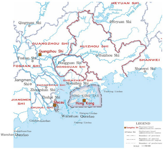
Figure 1.
Schematic diagram of the research area.
The Shenzhen metropolitan area is one of the most important developed metropolitan areas in China. High urbanization and motorization have led to changes in commuting modes and calls for urgent reductions in transportation carbon emissions This metropolitan area displays a typical spatial form of metropolitan areas, with a high population density and economic density in the center. Thus, the Shenzhen metropolitan area serves as a good representative for exploring carbon reduction from commuting in metropolitan areas.
3.2. Data Source
This study mainly uses Internet location data to obtain individual residence and employment information and uses a 3000 m × 3000 m grid as the basic data collection unit to calculate the commuting contact origin-destination (OD) within the Shenzhen metropolitan area. We choose this grid scale after fully considering data representativeness, calculation accuracy and the calculation amount. After multiple comparisons, the Internet location data are obtained through Baidu Maps for the period from 1 to 30 November 2019. Additionally, we adopt mobile signaling data from China Telecom as a supplement. The mobile signaling data are applied with the same grid scale and time periods as mentioned earlier. The road network data, bus stop data and land use type data are extracted from open street map. All the data are processed in terms of anonymization to ensure that there is no personal privacy or other relevant information involved.
The traditional data collection method involves obtaining the data of each administrative unit separately. The data obtained in this way are complete in terms of the internal links of cities. However, there are also deviations in the data consistency of the links between cities. The use of Internet data and mobile signaling data takes the Shenzhen metropolitan area as a complete geographical unit, and the data within this range are collected as a whole. Thus, these data can not only ensure the integrity of commuter contact data within cities in the Shenzhen metropolitan area but also ensure that the intercity contact data are accurate and comparable at the same level.
Existing studies show that daily travel patterns changed significantly during the COVID-19 pandemic, which started in 2020 [37]. China’s comprehensive COVID-19 lockdown was lifted in December 2022, and commuting activities in metropolitan areas are currently recovering. Therefore, we believe that although the data are not available for the most recent years, representative commuting characteristics can be obtained without the effect of the pandemic, which is also valuable for the future.
3.3. Variable Description
In this subsection, we introduce the variables used in our analysis and their definitions. Based on existing studies, the variables chosen can provide a relatively complete description of the factors influencing commuting carbon emissions from the perspectives of socioeconomics, public transportation services, and road networks. Thus, we take them into consideration in our analysis. We focus on the spatial heterogeneity of the influencing factors in this paper; therefore, some factors that are unable to reflect spatial heterogeneity at the grid level have been neglected. Moreover, factors such as the structure of public transport, the travel frequency and the travel distance have been used to calculate commuting carbon emissions. The effects are clear based on existing research. Therefore, these factors are not suitable as variables in our model.
As shown in Table 1, six indexes are selected to describe these factors in this paper: land-use diversity, location, the excess commuting rate, the commuting time spent on multiple means of public transport, the distance to the nearest bus stop and road network variables based on spatial design network analysis (sDNA) [38].

Table 1.
Selected variables.
3.3.1. Carbon Emission Variables
The Intergovernmental Panel on Climate Change (IPCC) model was proposed by the World Meteorological Organization (WMO) and the United Nations Environment Programme (UNEP) to calculate carbon emissions [39]. The calculation of carbon emissions is as follows:
where represents the data on emissions caused by the i-th type of human commuting activity and represents the coefficient used to quantify greenhouse gas emissions per unit activity. We adopt the carbon emission factor coefficients from the Beijing Municipal Ecology and Environment Bureau as shown in Table 2:
Table 2.
Carbon dioxide emissions per capita from different travel modes [40,41].
Thus, the carbon emissions from commuting are calculated as follows:
where represents the distance that the commuter moves using the i-th travel model and represents the coefficient used to quantify greenhouse gas emissions per unit activity. In this study, i equals 4, indicating 4 kinds of travel modes, which include private cars, buses, the metro and bicycles.
The distribution of carbon emissions is shown in Figure 2. Most of the high carbon emission regions of the three cities are located in peripheral areas, and the carbon emissions in the central areas are generally lower than those in the peripheral areas [33].
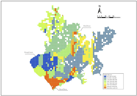
Figure 2.
Distribution of carbon emissions in three cities.
3.3.2. Land-Use Diversity
According to travel demand theories [42], mixed land uses place trip origins and destinations closer together and may therefore result in shorter commuting distances and less use of cars. Recent studies have shown that mixed land uses have a positive effect on reducing carbon emissions in general [43].
In this study, land-use diversity is calculated with land-use data from remote sensing impact identification. Shannon’s diversity index (SHDI) is used to measure land-use diversity. The calculation is shown below.
where H represents land-use diversity and represents the proportion of the i-th type of land use in the total. A higher value of H indicates a greater degree of land-use mixing.
3.3.3. Location
Location refers to the specific orientation of each grid in the Shenzhen metropolitan area. In this paper, we quantify location into three levels: “0” indicates that the grid is in the central area, “1” indicates that the grid is in the peripheral area, and “0.5” indicates that the grid is located between the central and peripheral areas of the metropolitan area. We adopt the “center”, “periphery”, and “in-between” classifications of the Commuting Observing Report in the Great Bay Area 2021 by the China Academy of Urban Planning and Design (CAUPD) [44].
3.3.4. Excess Commuting Rate
The excess commuting rate indicates the proportion of the actual commuting distance (ACD) exceeding the theoretical optimal commuting distance on average [44]. When the excess commuting rate is greater, the distance between the place of residence and the workplace is greater, which usually causes a longer commuting distance. Using the Baidu Map location service, information on travelers’ residences and employment locations is adopted to calculate the excess commuting rate.
Using the method proposed by Horner [45] and Ma [46], the excess commuting rate is calculated as follows:
First, the ACD is computed as follows:
where is the total number of commuting trips from home (h) to the workplace (j), is the commuting distance from home to the workplace, and T is the total number of commuting trips.
Then, we calculate the theoretical minimum commuting distance (MCD) as follows:
Subject to = = ≥ 0, where is the total number of commuting trips from origin h and is the total number of commuting trips to destination j.
The excess commuting rate is calculated using the ACD and MCD as follows:
excess commuting rate = (ACD − MCD)/ACD
3.3.5. Commuting Time Spent on Multiple Means of Public Transport
The commuting time spent on multiple means of public transport, which include the metro and buses, refers to the shortest travel time with public transport based on the street network using the Baidu Map application programming interface (API) for trip planning. The time spent includes the time to arrive at stations by walking, the waiting time, the riding time and the time needed for transfers by walking. This variable shows the public transport service level and transfer efficiency.
3.3.6. Distance to the Nearest Bus Stop
To evaluate the service level of bus facilities, we calculate the distance to the nearest bus stop at each grid central point with data extracted from open street map.
Recent research has shown that people may be more likely to take a bus when they are within 800 m of a bus stop, meaning that it may take them less than 10 min to reach the stop by walking [47]. Zhang and Zhou (2022) [48] also choose public transport accessibility (PTA), which indicates the number of bus stops within an 800 m radius of the place of residence, as a factor of carbon emissions. Therefore, we quantify the indexes with a binary indicator: “1” indicates that the distance to the nearest bus stop in the grid is within 800 m, while “0” indicates that the distance to the nearest bus stop in the grid is more than 800 m.
3.3.7. Road Network Attributes
Based on our previous work [33], in this paper, we mainly focus on integration parameters, which are calculated from the total number of nodes and the total depth of a node’s angle topology. Integration is often used to measure spatial permeability and centrality, and it includes two types of centralities:
Closeness centrality represents the accessibility of a street network to the rest of the street network within a given radius. In sDNA, closeness centrality is measured by the network quantity penalized by distance in radius angular (NQPDA), which is commonly referred to as a gravity model considering both the quantity and accessibility of the network weight.
where denotes the weight of node y in search radius for continuous space, and or 1 for discrete space. is the shortest topological distance from node to node . NQPDA(x) is the closeness centrality.
Betweenness centrality measures the probability that the street network has been circulated within a given radius. sDNA measures the two-phase betweenness (TPBt) of a destination by considering the competition between destinations to attract origins.
where represents the shortest topological path between node y and node z through node x in search radius R and denotes the total number of links. denotes the betweenness centrality, which represents the traversal of node x.
Two radii are chosen to compute closeness centrality and betweenness centrality. A radius of 2000 m is selected as the local scale. The radius of n, which is suitable for motor commuting, is selected as the global scale.
The list of all the variables is shown in Table 3.
Table 3.
List of the variables.
3.4. Analytical Approach
This paper uses 3000 m × 3000 m grids as the unit of analysis, which has been proven suitable for Chinese cities [49]. We take the average value of all variables as the value of each grid.
Notably, collinearity should be removed from the independent variables before using the GWR model. Thus, we first construct a stepwise regression model built through SPSS 26.0. In parallel, a GWR model built through ArcGIS 10.5 is used to analyze the impact of the independent variables on carbon emissions from commuting.
- (1)
- Stepwise regression model
Stepwise regression is a linear regression model-independent variable selection method. Its basic idea is to introduce variables one by one, and the condition of introduction is that the partial regression square sum experience is significant. At the same time, after each new variable is introduced, the existing variables that are not considered significant after testing are deleted. This process goes through several steps until no new variables can be introduced. All the variables in the regression model are significant for the dependent variable.
First, a monadic regression model is established:
, …, represent the values of the F test statistics of the corresponding regression coefficients. For a given significance level of 0.05, the corresponding critical value is marked as F(1). If ≥ F(1), then the variable should be introduced into the model. Ii represents the selected variable collection.
Second, a binary regression model of dependent variable Y and independent variable subset {, X1}, …, {, Xi1−1}{, }, …, {, Xp} is established. Additionally, the value of the F test statistic of the corresponding regression coefficient is calculated as (k), which is not included in I1.
For a given significance level of 0.05, the corresponding critical value is marked as F(2). If ≥ F(2), then the variable should be introduced into the model. Otherwise, the variable introduction process should be terminated.
Finally, this method is repeated. We select one of the independent variables that has not been introduced into the regression model each time until no variables remained.
- (2)
- Geographically weighted regression model
The GWR model is an important tool for exploring spatial heterogeneity. The regression parameters in the linear regression model are generalized as functions of spatial position coordinates. Based on the local additive, weighted least squares estimation fitting model, the local estimation of the coefficient function at each geographical location is used to characterize the characteristics and influence of the corresponding independent variable on the dependent variable with the change in geographical location.
where (u,v) (j = 1,2, …, p) represents the regression coefficient function at point (u,v). { is the random error and is assumed to be independent, E(.
Additionally, the results for carbon emissions, the commuting time spent on multiple means of public transport and the excess commuting rate are calculated based on OD information.
4. Results
4.1. Results of the Stepwise Regression Model
Table 4 summarizes the variables that pass the significance test after 3 steps in the stepwise regression model. The R-square of the final model is 0.551 (see Table 5). Table 6 shows the coefficients of the variables ultimately retained and the variance inflation factor (VIF) results.
Table 4.
Summary of the independent variables used in the proposed models. Note: √ in the table means the independent variable has been chosen, while × means the variable has been neglected.
Table 5.
Summary of the final model (Model 3).
Table 6.
Coefficients of the final model (Model 3).
Note that the independent variables of Model 3 are determined based on the stepwise regression of the other two models.
The results help us identify the key factors that are suitable for GWR analysis. Our results indicate that land-use diversity, location, the excess commuting rate, and the distance to the nearest bus stop are significantly correlated with carbon emissions from commuting. In addition, the stepwise regression model results confirm the impact of street network variables on carbon emissions from commuting. Specifically, global (R = n) closeness centrality is significantly positively correlated with carbon emissions from commuting. Areas that have greater potential to attract traffic flow may generate more carbon emissions. Furthermore, local (R = 2 km) betweenness centrality has a significant negative impact on carbon emissions, which means that the easier the area is to pass through, the fewer carbon emissions are generated. Meanwhile, the impact of betweenness centrality on carbon emissions is smaller than that of closeness centrality. Overall, the stepwise regression results indicate that network attributes are key factors influencing commuting carbon emissions and could be carefully considered in spatial heterogeneity analysis.
4.2. Results of the Geographically Weighted Regression Model
According to the ordinary least squares model generated through ArcGIS, the Koenker–Bassett test is significant, indicating that the independent variables have spatial heterogeneity and are suitable for the GWR model. On the basis of the stepwise regression results, we further remove the independent variables with collinearity in GWRs, which include location, the commuting time spent on multiple means of public transport, global closeness centrality (R = n), and local closeness centrality (R = 2000 m). Finally, five variables remain in the next-step spatial heterogeneity analysis, namely, the excess commuting rate, the distance to the nearest bus stop and land-use diversity, local betweenness centrality (R = 2000 m), and global betweenness centrality (R = n). The results of the GWR model are shown in Figure 3, and the standard errors of this model are shown in Figure 4.
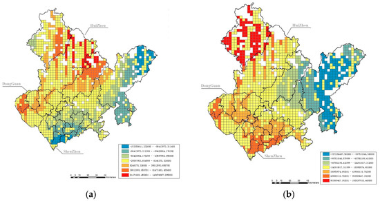

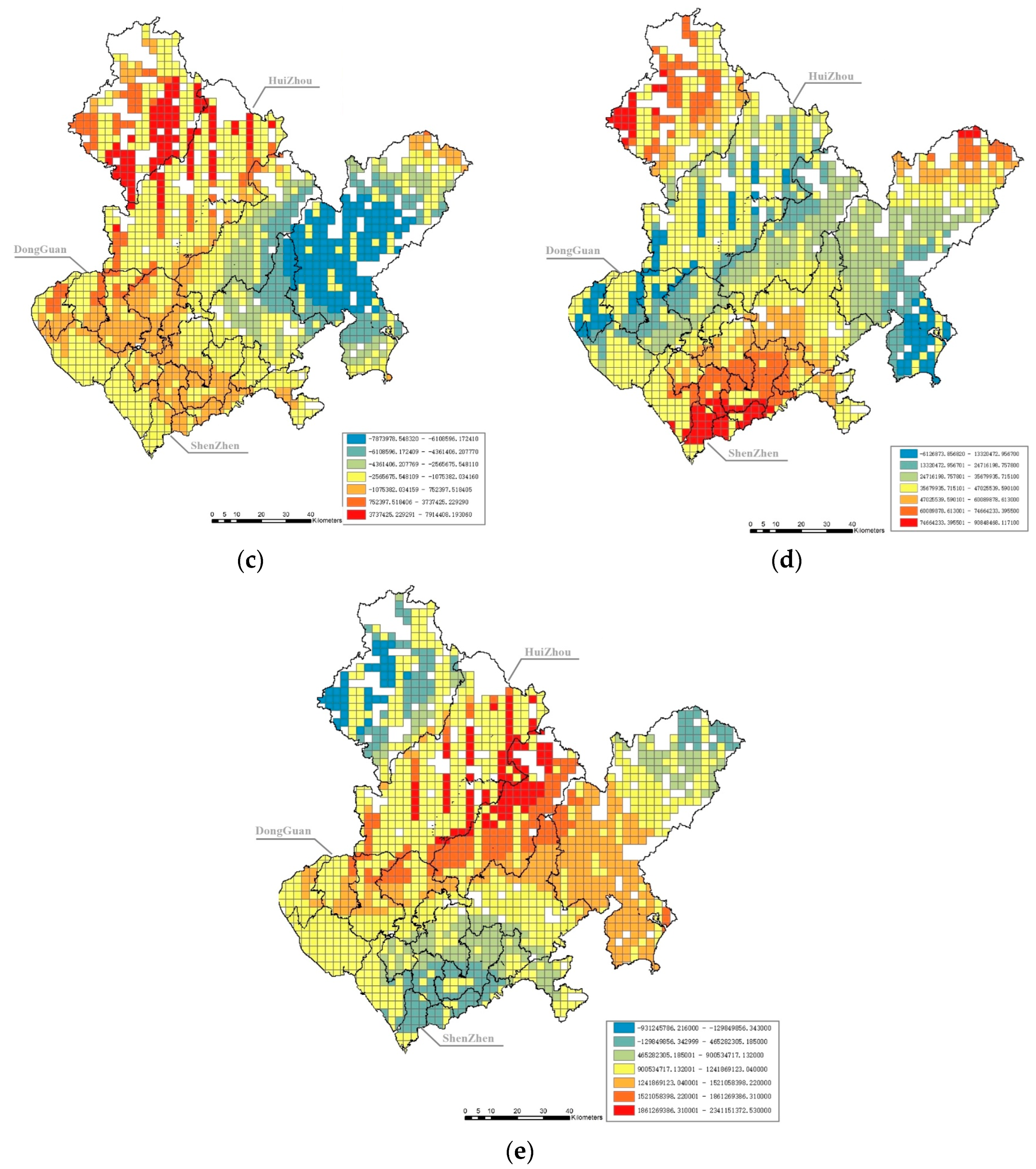
Figure 3.
Coefficient results of the GWR model at the grid level. Note: The boundary lines of cities and districts are schematic. (a) shows the impact coefficient of land-use diversity on carbon emissions. (b) shows the coefficient of the impact of the excess commuting rate on carbon emissions. (c) shows the coefficient of the impact of the distance to the nearest bus stop on carbon emissions. (d) shows the coefficient of the impact of local betweenness centrality (R = 2 km) on carbon emissions. (e) shows the coefficient of the impact of global betweenness centrality (R = n) on carbon emissions.
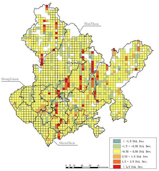
Figure 4.
Standard error results at the grid level. Note: The boundary lines of cities and districts are schematic.
The standard error shown in Figure 4 indicates that most of the grids have a good fit to the model. The results of the GWR model should be effective and interpretable as follows.
First, it is obvious that land-use diversity has a significant negative effect on carbon emissions in general, especially in the center of Shenzhen. However, in Dongguan and the western part of Huizhou, the effects are the opposite. The center of Shenzhen has the highest population and job density in the metropolitan area, and mixed land uses may easily increase the likelihood of working nearby and decrease carbon emissions from commuting.
Second, the results show that the excess commuting rate and the distance to the nearest bus stop have uncertain effects on carbon emissions in different grids. In Dongguan and part of Shenzhen, a higher excess commuting rate may lead to higher carbon emissions. In Huizhou and the periphery of Shenzhen, the shorter the distance to the nearest bus stop is, the lower the carbon emissions. The uncertainty may be related to the metro service level; areas with lower metro coverage prefer bus services, and there is a close connection between the bus service level and carbon emissions.
Finally, the results also suggest that the influence degree of betweenness centrality is distributed in circles. Local (R = 2 km) betweenness centrality has a negative impact on carbon emissions in peripheral areas. One possible reason is that the road network is inadequate in peripheral areas and has many broken roads at the boundaries of cities; a road network that is easier and quicker to pass through may lead to fewer carbon emissions. Global (R = n), betweenness centrality is negatively correlated with carbon emissions in Shenzhen but has a positive impact in most parts of Dongguan and Huizhou. Although Shenzhen has a greater potential to attract traffic flow than Dongguan and Huizhou, the metro and bus services of Shenzhen are much better than those of the other two cities. Thus, the high global (R = n) betweenness centrality in Shenzhen may generate more public transport use and fewer carbon emissions.
5. Conclusions and Discussion
5.1. Conclusions
Although there are differences in the terrain and landscape of different metropolitan areas, the characteristics of commuting in developed metropolitan areas have significant similarities, including large-scale commuting from the center to the periphery and across city boundaries. The issue of transportation facilities also has commonalities, for example, the lack of public service on the periphery. Like other metropolises, the Shenzhen metropolitan area has major concentrations of energy use and carbon emissions; thus, studies are needed to explore how to identify the factors influencing carbon emissions and reduce carbon emissions. The main purpose of this research is to explore new methods for studying commuting carbon emissions at the level of metropolitan areas through the usage of big data. The second purpose is to reveal the spatial characteristics of carbon emissions based on factors from a comprehensive perspective and to provide constructive suggestions for policymakers.
The factors discussed in our study, including the excess commuting rate, the distance to the nearest bus stop, land-use diversity, local betweenness centrality (R = 2000 m), and global betweenness centrality (R = n), exhibit significant spatial heterogeneity with different layers of the metropolitan area. Our findings indicate that carbon emissions from commuting are positively correlated with global closeness centrality and negatively correlated with global betweenness centrality, which is considered an innovative perspective. Our results also reveal that the higher the excess commuting rate is, the greater the carbon emissions from commuting, while land-use diversity has a significant negative correlation with carbon emissions. In addition, in most parts of the metropolitan area, a shorter distance to the nearest bus stop will result in lower carbon emissions.
5.2. Discussion
Based on our findings, several important implications are discussed below.
First, our work highlights the influence of road network attributes, and our findings indicate that carbon emissions may be greater if the road has more possibilities to attract cars. In contrast, if vehicles simply pass through a road smoothly, without stopping, carbon emissions should decrease. It has also been confirmed that carbon emissions are relatively low when vehicles move at a steady, medium speed [50]. The main reason may be that street centrality affects idle vehicles. To lower carbon emissions from commuting, governments should improve road network connectivity, especially in border areas between cities where unified road planning is often lacking.
Second, land-use diversity is an influential factor according to our stepwise regression model results. According to a previous study [51], high land-use heterogeneity decreases travel distances and facilitates energy-efficient transport modes, and personal income and demographics are the most influential individual-level factors. There is a higher population density and higher average salaries in the center of Shenzhen [52], where land-use diversity has a significant negative correlation with carbon emissions. Our results also show that higher excess commuting results in higher carbon emissions from commuting. A high excess commuting rate indicates that the real commuting distance in the region is greater than the optimal distance, reflecting an unbalanced distribution of workplace and residence locations. This unbalanced residence and workplace distribution may cause long commuting distances, which will further generate higher commuting carbon emissions. Therefore, policymakers should encourage land-use diversity to reduce carbon emissions, especially in the center of metropolitan areas. Affordable housing for talent should also be considered an appropriate layout in the central area, which may help reduce long-distance commuting in the central area and decrease carbon emissions.
Third, the GWR model demonstrates that the influence degree (coefficient) is significantly diverse in different layers of the metropolitan area. In the center of the Shenzhen metropolitan area, there is a high population density, personal income and commuting demand, which generate more carbon emissions. Meanwhile, the closer a geographical location is to city boundaries, the greater the carbon emissions in general. In addition, we find that for most parts of the metropolitan area, when the distance to the nearest bus stop is 800 m, more commuters will be likely to take the bus to work. The bus service level on the periphery of metropolitan areas affects carbon emissions more than does that in the central area. Due to the lack of public transport in the periphery of metropolitan areas, most trips on the periphery need to depend on motor vehicles. However, this does not automatically mean that any location in the peripheral area will have high carbon emissions; the main traffic modes of some peripheral areas are walking and cycling, resulting in lower carbon emissions. Overall, public transport facilities and service levels in peripheral areas are more important. Improving public transport and rail transit across cities in metropolitan areas should receive increased attention from governments.
Based on the findings above, this paper also provides implications and policy suggestions for sustainable commuting modes in the future. First, urban congestion should be alleviated by optimizing the road network, eliminating dead-end roads, and reducing car congestion, especially on the periphery of metropolitan areas. Keeping the car speed at a normal level, rather than at an extreme level, helps effectively reduce carbon emissions from commuting. Second, the mixed use of land contributes to reducing carbon emissions from commuting, especially in the center of metropolitan areas. Thus, approaches such as building residences around central business districts and improving the balance between residences and workplaces could be effective in reducing carbon emissions. Third, a sustainable public transport system should be built to attract more commuters. The coverage of public transport should be especially improved in peripheral regions. Fourth, policymakers should consider the spatial heterogeneity of variables and develop suitable policies to adapt to the conditions of different layers in metropolitan areas.
5.3. Limitations and Recommendations for Future Studies
This study is not without limitations. First, the road network variables are based on space syntax theory, which is just a topological network analysis. Although we carefully selected the most important factors in our model, additional relevant factors could be explored further. Moreover, future research could investigate the impacts on carbon emissions from commuting with a dynamic perspective by exploring the differences in emissions during different time periods. Second, we obtained data for only one month, which may be less than the ideal length; moreover, the data sources are not diverse enough due to data accessibility. This issue could be addressed in future research with additional data sources. Finally, although we believe that the Shenzhen metropolitan area is representative of other developed metropolitan areas, comparisons with other metropolitan areas are lacking, which could be addressed in future studies.
Author Contributions
Conceptualization, X.L.; methodology, X.L.; software, J.Z.; formal analysis, W.Z.; resources, J.Z.; data curation, J.Z. and W.Z.; writing—original draft preparation, X.L.; writing—review and editing, Y.T.; funding acquisition, Y.T. All authors have read and agreed to the published version of the manuscript.
Funding
This work was supported by the Shenzhen Stable Support Plan Program for Higher Education Institutions [Grant Number: 20220815113158002].
Institutional Review Board Statement
Not applicable.
Informed Consent Statement
Written informed consent has been obtained from the patient(s) to publish this paper.
Data Availability Statement
We declare that the data used in this paper is purchased by China Academy of Urban Planning and Design and cannot be disclosed publicly.
Acknowledgments
Yue Tan acknowledges the support of Shenzhen Stable Support Plan Program for Higher Education Institutions (Grant Number: 20220815113158002).
Conflicts of Interest
The authors declare no conflict of interest.
References
- The White House, United States Mid-Century Strategy for Deep Decarbonization. Available online: https://unfccc.int/files/focus/long-term_strategies/application/pdf/mid_century_strategy_report-final_red.pdf (accessed on 1 November 2016).
- Japanese Ministry of Environment. CO2 Emission Factors of Different Fuels; Japanese Ministry of Environment: Tokyo, Japan, 2019.
- BBC News. Climate Change: China Aims for ‘Carbon Neutrality by 2060’. Available online: https://www.bbc.com/news/science-environment-54256826 (accessed on 27 November 2021).
- Notte, A.L.; Tonin, S.; Lucaroni, G. Assessing direct and indirect emissions of greenhouse gases in road transportation, taking into account the role of uncertainty in the emissions inventory. Environ. Impact Assess. Rev. 2018, 69, 82–93. [Google Scholar] [CrossRef]
- Zhang, W.; Qi, Y.; Yan, Y.; Tang, J.; Wang, Y. A method of emission and traveller behavior analysis under multimodal traffic condition. Transp. Res. Part D Transp. Environ. 2017, 52, 139–155. [Google Scholar] [CrossRef]
- Wang, H.; Zeng, W. Revealing urban carbon dioxide (CO2) emission characteristics and influencing mechanisms from the perspective of commuting. Sustainability 2019, 11, 385. [Google Scholar] [CrossRef]
- Fang, J.; Meng, X.; Tian, J.; Xing, C.; Wang, C.; Wood, J. A review of transportation carbon emissions research using bibliometric analyses. J. Traffic Transp. Eng. 2023, 10, 5. [Google Scholar] [CrossRef]
- Andersen, P.H.; Mathews, J.A.; Rask, M. Integrating private transport into renewable energy policy: The strategy of creating intelligent recharging grids for electric vehicles. Energy Policy 2009, 37, 2481–2486. [Google Scholar] [CrossRef]
- Sorrell, S. Reducing energy demand: A review of issues, challenges and approaches. Renew. Sustain. Energy Rev. 2015, 47, 74–82. [Google Scholar] [CrossRef]
- You, F.; Hu, D.; Zhang, H.; Guo, Z.; Zhao, Y.; Wang, B.; Yuan, Y. Carbon emissions in the life cycle of urban building system in China—A case study of residential buildings. Ecol. Complex. 2011, 8, 201–212. [Google Scholar] [CrossRef]
- Cao, X.; Yang, W. Examining the effects of the built environment and residential self-selection on commuting trips and the related CO2 emissions: An empirical study in Guangzhou, China. Transp. Res. Part D Transp. Environ. 2017, 52, 480–494. [Google Scholar] [CrossRef]
- Chow, A.S.Y. Spatial-modal scenarios of greenhouse gas emissions from commuting in Hong Kong. J. Transp. Geogr. 2016, 54, 205–213. [Google Scholar] [CrossRef]
- Reznik, A.; Kissinger, M.; Alfasi, N. Real-data-based high-resolution GHG emissions accounting of urban residents private transportation. Int. J. Sustain. Transp. 2019, 13, 235–244. [Google Scholar] [CrossRef]
- Zhang, X.; Liu, P.; Li, Z.; Yu, H. Modeling the effects of low-carbon emission constraints on mode and route choices in transportation networks. Procedia Soc. Behav. Sci. 2013, 96, 329–338. [Google Scholar] [CrossRef]
- Xia, C.; Xiang, M.; Fang, K.; Li, Y.; Ye, Y.; Shi, Z.; Liu, J. Spatial-temporal distribution of carbon emissions by daily travel and its response to urban form: A case study of Hangzhou, China. J. Clean. Prod. 2020, 257, 120797. [Google Scholar] [CrossRef]
- Chen, C.; Zhen, F.; Huang, X. How does perceived neighborhood environment affect commuting mode choice and commuting CO2 emissions? An empirical study of Nanjing, China. Int. J. Environ. Res. Public Health 2022, 19, 7649. [Google Scholar] [CrossRef]
- Wang, Y.; Yang, L.; Han, S.; Li, C.; Ramachandra, T.V. Urban CO2 emissions in Xi’an and Bangalore by commuters: Implications for controlling urban transportation carbon dioxide emissions in developing countries. Mitig. Adapt. Strategies Glob. Chang. 2017, 22, 993–1019. [Google Scholar] [CrossRef]
- Ewing, R.; Cervero, R. Travel and the built environment: A synthesis. Transp. Res. Rec. 2001, 1780, 87–114. [Google Scholar] [CrossRef]
- Wang, Z.; Chen, F.; Taku, F. Carbon emission from urban passenger transportation in Beijing. Transp. Res. Part D Transp. Environ. 2015, 41, 217–227. [Google Scholar] [CrossRef]
- Li, S.; Xue, F.; Xia, C.; Zhang, J.; Bian, A.; Liang, Y.; Zhou, J. A big data-based commuting carbon emissions accounting method—A case of Hangzhou. Land 2022, 11, 900. [Google Scholar] [CrossRef]
- Akshima, T.G.; Sharif, Q. Carbon footprint of urban public transport systems in Indian cities. Case Stud. Transp. Policy 2020, 8, 245–251. [Google Scholar]
- Dong, D.; Duan, H.; Mao, R.; Song, Q.; Zuo, J.; Zhu, J.; Wang, G.; Hu, M.; Liu, G. Towards a low carbon transition of urban public transport in megacities: A case study of Shenzhen, China. Resour. Conserv. Recycl. 2018, 134, 149–155. [Google Scholar] [CrossRef]
- Zhang, L.; Long, R.; Chen, H.; Yang, T. Analysis of an optimal public transport structure under a carbon emission constraint: A case study in Shanghai, China. Environ. Sci. Pollut. Res. 2018, 25, 3348–3359. [Google Scholar] [CrossRef] [PubMed]
- Jiang, Y.; Zhou, Z.; Liu, C. The impact of public transportation on carbon emissions: A panel quantile analysis based on Chinese provincial data. Environ. Sci. Pollut. Res. 2019, 26, 4000–4012. [Google Scholar] [CrossRef] [PubMed]
- Shu, Y.; Lam, N.S.N. Spatial disaggregation of carbon dioxide emissions from road traffic based on multiple linear regression model. Atmos. Environ. 2011, 45, 634–640. [Google Scholar] [CrossRef]
- Wang, J.; Li, P.; Gao, J. Region division in China for transportation carbon emission reduction. J. Chang. Univ. 2012, 32, 72–79. [Google Scholar]
- Wu, R.; Zhang, J.; Bao, Y.; Zhang, F. Geographical detector model for influencing factors of industrial sector carbon dioxide emissions in inner Mongolia, China. Sustainability 2016, 8, 149. [Google Scholar] [CrossRef]
- Lu, X.; Ota, K.; Dong, M.; Yu, C.; Jin, H. Predicting transportation carbon emission with urban big data. IEEE Trans. Sustain. Comput. 2017, 2, 333–344. [Google Scholar] [CrossRef]
- Ashik, F.R.; Rahman, M.H.; Antipova, A.; Zafri, N.M. Analyzing the impact of the built environment on commuting-related carbon dioxide emissions. Int. J. Sustain. Transp. 2023, 17, 258–272. [Google Scholar] [CrossRef]
- Rahman, M.H.; Islam, M.H.; Neema, M.N. GIS-based compactness measurement of urban form at neighborhood scale: The case of Dhaka, Bangladesh. J. Urban Manag. 2021, 11, 6–22. [Google Scholar] [CrossRef]
- Alam, S.; Kumar, A.; Dawes, L. Roughness optimization of road networks: An option for carbon emission reduction by 2030. J. Transp. Eng. Part B Pavements 2020, 146, 04020062. [Google Scholar] [CrossRef]
- Yamagata, Y.; Murakami, D.; Wu, Y.; Yang PP, J.; Yoshida, T.; Binder, R. Big-data analysis for carbon emission reduction from cars: Towards walkable green smart community. Energy Procedia 2019, 158, 4292–4297. [Google Scholar] [CrossRef]
- Zhang, J.; Yang, Y.; Li, X. The Impact of Street Network Structure on Carbon Emissions from Commuting Evidence from Three Chinese Cities. In Proceedings of the 13th Space Syntax Symposium, Bergen, Norway, 20–24 June 2022; Available online: https://www.hvl.no/globalassets/hvl-internett/arrangement/2022/13sss/340zhang.pdf (accessed on 20 June 2022).
- Liu, Z.; Sun, T.; Yu, Y.; Ke, P.; Deng, Z.; Lu, C.; Huo, D.; Ding, X. Real-Time Carbon Emission Accounting Technology toward Carbon Neutrality. Engineering 2022, 14, 44–51. [Google Scholar] [CrossRef]
- Li, S.; Zhao, P. Examining Commuting Disparities across Different Types of New Towns and Different Income Groups: Evidence from Beijing, China. Habitat Int. 2022, 124, 102558. [Google Scholar] [CrossRef]
- Guangdong Provincial Development and Reform Commission. Overall Development Plan of Guangdong Development Zone; Guangdong Provincial Development and Reform Commission: Guangzhou, China, 2020. [Google Scholar]
- James, D.W.; Léa, R.; Ahmed, E.G. Travel behaviour and greenhouse gas emissions during the COVID-19 pandemic: A case study in a university setting. Transp. Res. Interdiscip. Perspect. 2022, 13, 100531. [Google Scholar] [CrossRef]
- Cooper, C. Spatial Design Network Analysis (sDNA) Manual—sDNA 4.0.2 Documentation. Available online: https://sdna.cardiff.ac.uk/sdna/wp-content/downloads/documentation/manual/sDNA_manual_v4_0_2/ (accessed on 19 December 2021).
- Intergovernmental Panel on Climate Change. Guidelines for National Greenhouse Gas Emission Inventories; Intergovernmental Panel on Climate Change: Geneva, Switzerland, 2020. [Google Scholar]
- Shenzhen Municipal People’s Government. Carbon Inclusion Methodology of Low Carbon Public Travel in Shenzhen. 2021. Available online: http://meeb.sz.gov.cn/attachment/0/927/927134/9442897.pdf (accessed on 1 December 2021).
- Beijing Municipal Bureau of Ecology and Environment. Methodology for Low-carbon Travel and Carbon Emission Reduction in Beijing (Trial Version). 2020. Available online: http://sthjj.beijing.gov.cn/bjhrb/index/xxgk69/zfxxgk43/fdzdgknr2/zcfb/hbjfw/2020/1758471/2020041317265121877.docx (accessed on 1 April 2020).
- Lu, H.P. Theory and Method in Transportation Planning; Tsinghua University Press: Beijing, China, 2009. [Google Scholar]
- Song, Y.; Louis, M.; Daniel, R. Comparing measures of urban land use mix. Comput. Environ. Urban Syst. 2013, 42, 1–13. [Google Scholar] [CrossRef]
- China Academy of Urban Planning and Design. Commuting Observing Report in the Great Bay Area; China Academy of Urban Planning and Design: Beijing, China, 2021. [Google Scholar]
- Horner, M.W. Spatial dimensions of urban commuting: A review of major issues and their implications for future geographic research. Prof. Geogr. 2004, 56, 160–173. [Google Scholar] [CrossRef]
- Ma, K.R.; Banister, D. Excess commuting: A critical review. Transp. Rev. 2006, 26, 749–767. [Google Scholar] [CrossRef]
- Ahmed, E.G.; Grimsrud, M.; Wasfi, R.; Tétreault, P.; Surprenant-Legault, J. New evidence on walking distances to transit stops: Identifying redundancies and gaps using variable service areas. Transportation 2014, 41, 193–210. [Google Scholar]
- Zhang, Y.; Zhou, W.; Ding, J. Effects of the built environment on travel-related CO2 emissions Considering Travel purpose: A case study of resettlement neighborhoods in Nanjing. Buildings 2022, 12, 1718. [Google Scholar] [CrossRef]
- Gu, H.; Shen, T.; Zhou, L.; Chen, H.; Xiao, F. Measuring street layout’s spatio-temporal effects on housing price based on GWR and sDNA model: The case study of Guangzhou. Econ. Geogr. 2018, 38, 82–91. [Google Scholar]
- Boriboonsomsin, K.; Barth, M. Impacts of road grade on fuel consumption and carbon dioxide emissions evidenced by use of advanced navigation systems. Transp. Res. Rec. 2009, 2139, 21–30. [Google Scholar] [CrossRef]
- Zhang, M.; Zhao, P. The impact of land-use mix on residents’ travel energy consumption: New evidence from Beijing. Transp. Res. Part D Transp. Environ. 2017, 57, 224–236. [Google Scholar] [CrossRef]
- Southern Human Resources Evaluation Center; Guangzhou Talent Research Institute; Guangzhou Wangcai Information Technology Co., Ltd.; Guangzhou Human Resources Service Association. 2023–2024 Guangdong Province Salary Survey Report; Nan Fang Daily: Guangzhou, China, 2023. [Google Scholar]


Disclaimer/Publisher’s Note: The statements, opinions and data contained in all publications are solely those of the individual author(s) and contributor(s) and not of MDPI and/or the editor(s). MDPI and/or the editor(s) disclaim responsibility for any injury to people or property resulting from any ideas, methods, instructions or products referred to in the content. |
© 2024 by the authors. Licensee MDPI, Basel, Switzerland. This article is an open access article distributed under the terms and conditions of the Creative Commons Attribution (CC BY) license (https://creativecommons.org/licenses/by/4.0/).