Spatiotemporal Characteristics and Driving Factors of Ecosystem Regulation Services Value at the Plot Scale

Abstract

The value of ecosystem regulation services (ERSV) is a crucial aspect of gross ecosystem product (GEP). Understanding and mastering the spatiotemporal evolution characteristics and driving factors of ERSV is essential for the efficient management of regional ecosystems. This study proposes an ERSV accounting model at the plot scale and uses the barycentric analysis method, the optimal parameters-based geographical detector model (OPGD), and the constraint line extraction method to analyze the spatiotemporal evolution characteristics, main driving factors, and constraint rules of ERSV in Yunyang District, Hubei Province in 2016, 2018, 2020, and 2021. The results show that (1) In the temporal dimension, the overall ERSV of the district increased by CNY 1.664 billion from 2016 to 2021, with an increase rate of 3.68%. The contribution values of climate regulation function and water retention function to ERSV was significant. (2) In the spatial dimension, the ERSV was high in the north and south and low in the middle, with high-value areas mainly located in woodland and wetland areas. The center of gravity of the ERSV increase shifted to the southwest by 12,455.42 m, while the center of gravity of the reduction shifted to the southwest by 3582.79 m from 2016 to 2021. (3) The interaction of any two driving factors had greater explanatory power for the spatial differentiation of ERSV than that of a single driving factor, and all of them showed nonlinear or double factor enhancement characteristics. The human active index (HAI) and construction land proportion (CLP) were the leading anthropogenic factors, while the land surface temperature (LST) and NDVI were the leading natural factors. (4) The ERSV could maintain a high and stable value output when the HAI was less than 0.3, CLP was less than 15%, LST was between 18 and 22 °C, and NDVI was greater than 0.5. These results can guide the practices of ecology, production, and life in Yunyang District and contribute to the high quality and sustainable development of the regional ecology and economy.

1. Introduction

The ecosystem provides both material and non-material benefits for human beings, supporting their survival and development [1,2]. Research on ecosystem services (ESs) and ecosystem services value (ESV) accounting has become a hot topic in current ecology and ecological economics research [3,4,5,6]. In recent years, under the guidance of General Secretary Xi Jinping’s theory that “lucid waters and lush mountains are invaluable assets”, China has made significant efforts to promote the construction of an ecological civilization, explicitly requiring that ecological benefits be included in the evaluation index system for the government and cadres. Protecting the ecological environment and creating a green home are seen as essential for current economic development [7,8]. In order to evaluate the contribution of ecosystems to human well-being and the sustainable development of the economy and society, Ouyang et al. [9] proposed an indicator for evaluating this contribution—the gross ecosystem product (GEP)—based on the concept of gross domestic product (GDP). This refers to the sum of the ecosystem material product value (EMPV), ecosystem regulation services value (ERSV), and ecological culture services value (ECSV) provided by various ecosystems in a certain region during a specific accounting period.

As an important component of GEP, the indirect benefits provided by ERSV far exceed the direct value [10], accounting for more than 70% and even up to 90% of GEP in areas rich in ecological resources such as forests [11,12,13]. However, despite its significant contribution, the role of ERSV has been overlooked for a long time, with an excessive focus on and consumption of EMPV and ECSV. This has resulted in the degradation of the ecological environment [14,15] and the decline in ESs [16], prompting extensive research on the spatiotemporal evolution characteristics and driving factors of ESs by both domestic and foreign scholars [17,18,19].

In current research, GEP accounting and difference analysis are typically conducted at the city, county, township, and village levels based on administrative division units [20,21,22,23]. However, this approach fails to reveal the internal spatial differences due to the lack of precision in the basic units of accounting [24]. Additionally, GEP accounting studies using different grid scales based on the resolution of land use raster data have encountered various issues [25,26], such as the complexity of the accounting process by ecosystem type and the potential for classification errors in the land use raster data, which can increase the uncertainty of GEP assessment [27]. Furthermore, due to the availability of data, there are few reports on the accounting and comprehensive comparative analysis of GEP at the county level and long time series and plot scale, and the spatiotemporal characteristics and driving factors of GEP are not clear.

In view of this, and considering the important role of ERSV and the impact of continuous data access, this study focuses on the Yunyang District of Hubei Province and utilizes a refined land remote sensing intelligent interpretation algorithm to accurately identify and process the third land survey data, resulting in fine ecological plot data for the study area. This allows for the development of an ERSV accounting model at the plot scale. The study then delves into the spatiotemporal evolution characteristics, driving factors, and constraint rules of ERSV at the plot scale in Yunyang District, Hubei Province, with the aim of providing a more scientific and robust basis for decision-making in regional territorial space optimization management, ecological environment protection and restoration, and the realization of ecological product value.

2. Material and Methods

2.1. Study Area

Yunyang District (32°25′–33°16′ N, 110°07′–111°16′ E) is located in the northwest of Hubei Province and is part of Shiyan City. It encompasses 16 towns, 3 townships, and 1 forest farm (Figure 1), with a total area of 3863 km². The district is situated between the southern slope of the Qinling Mountains and the eastern extension of the Daba Mountains, with a varied terrain of high and low areas and an altitude ranging from 1066 to 1805 m. The climate in this region is subtropical and humid, with an average annual precipitation of 824 mm and an average annual temperature of 13–16 °C. The abundant precipitation and suitable temperature contribute to the rich water resources in Yunyang District. Additionally, the district has well-developed water systems and is a key water source area for the Central Line Project of South-to-North Water Diversion. The forest coverage rate in this region is 66.87%, indicating abundant forest resources. Furthermore, the district boasts over 93% of days with good air quality, making it an important contributor to climate regulation, water retention, and water environment purification.

2.2. Data Source and Processing

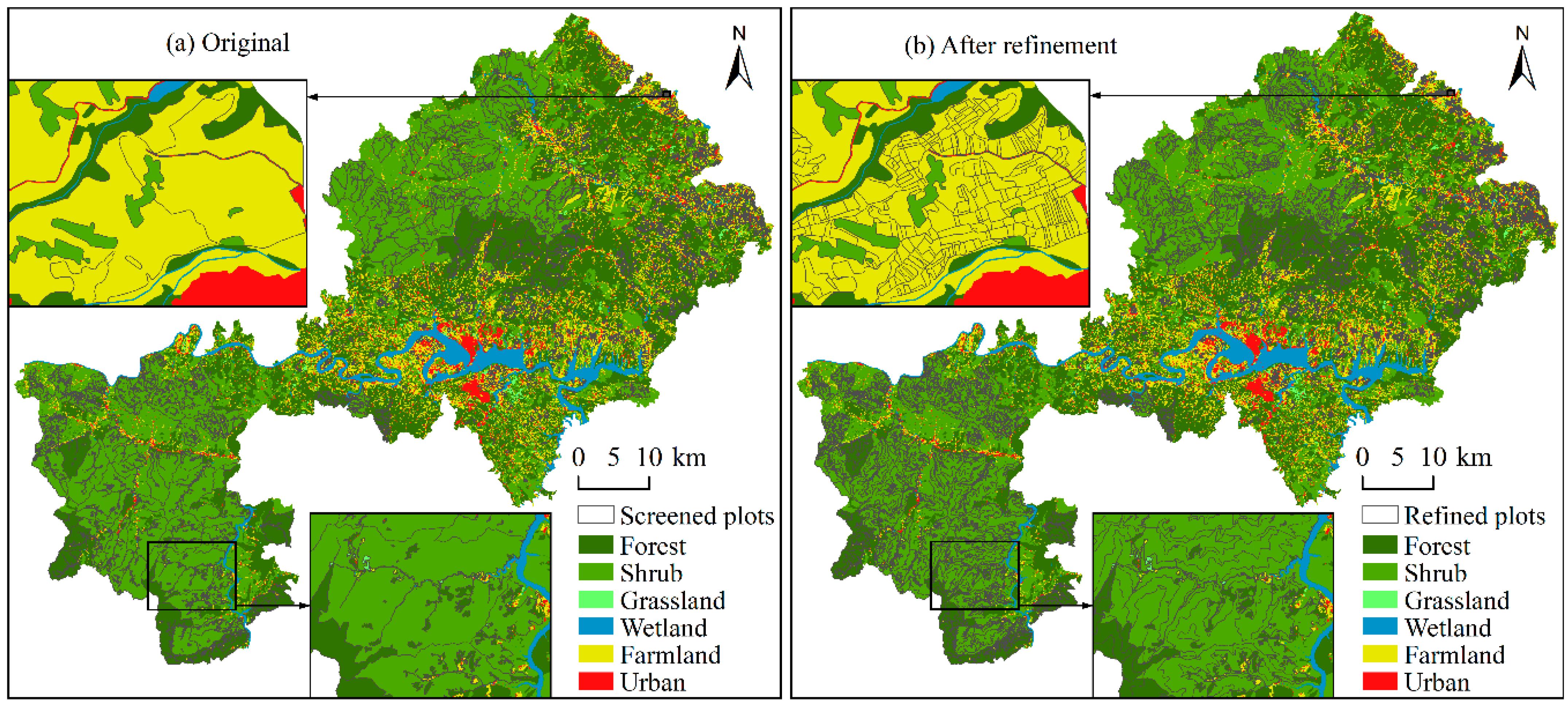
2.2.1. Ecological Plot Data

Based on the land use survey data provided by the land resources department of Yunyang District, detailed ecological plot data were obtained. First, the important role of cultivated land, garden land, forest land, and grassland in human production and life, as well as their significant contribution to ESV [28,29], were considered. Plots of cultivated land with an area greater than 0.1 km² and plots of garden, forest land, and grassland with an area greater than 3 km² were selected. Next, the intelligent remote sensing interpretation algorithm for fine plots was used to accurately identify and process the large area plots. Finally, the ecological plot data with geographic entity unit information were obtained through manual modification and matching with ecosystem types. This study produced ecological plot data for the years 2016, 2018, 2020, and 2021. The number of plot spots before and after refinement in each year is shown in

Table 1. The overview of the ecological plot before and after the refinement of land use data from 2016 to 2021.

Year	Number of the Original Plots	Number of the Screened Plots	Number of Plots after Refinement	Minimum Plot Area/m2
2016	62,772	1132	111,278	30.34
2018	65,100	1089	113,836	31.06
2020	105,730	722	118,325	30.80
2021	106,132	586	119,211	30.32

, and comparison examples can be seen in Figure 2.

2.2.2. Driving Factors and Accounting Index Parameter Data

In this study, we have selected both anthropogenic and natural drivers that may impact the spatial differentiation of regional ERSV. We have referenced previous research on the drivers of ESV in Hubei Province [30,31] and have taken into account the specific circumstances of Yunyang District, as well as the availability of continuous data on driving factors. We have identified three anthropogenic and five natural driving factors. The anthropogenic factors include the human activity index (HAI), population density (POPD), and construction land proportion (CLP). The natural factors include the annual precipitation (PRE), digital elevation model (DEM), average annual normalized difference vegetation index (NDVI), average annual land surface temperature (LST), and annual evapotranspiration (ET). The details of these factors are listed in

Table 2. Construction of an index system for the driving force of the spatial heterogeneity of ERSV in Yunyang District, Hubei Province.

Type	Factors	Resolution	Year	Data Source and Processing
Anthropogenic factor	HAI	100 m	2016 2018 2020 2021	The mathematical model constructed by Yan et al. [32] was used for calculation based on the ecological plot data and rasterized to 100 m × 100 m.
	POPD/(person·km−2)	1 km		Based on the LandScan Global Population Data (https://landscan.ornl.gov/) (accessed on 11 July 2023), and the vector border of the Yunyang District was used to extract the mask.
	CLP/%	1 km		The proportion of construction land in the area of each 1 km × 1 km fishing net unit was calculated based on ArcGIS10.8 software.
Natural factor	DEM/m	30 m	2019	Based on the ASTER GDEM V3 data provided by the Geospatial Data Cloud (http://www.gscloud.cn/) (accessed on 6 September 2022), and the vector border of the Yunyang District was used to extract the mask.
	PRE/mm	1 km	2016 2018 2020 2021	Based on the 1 km monthly precipitation dataset for China provided by the National Tibetan Plateau Scientific Data Center (https://data.tpdc.ac.cn/) (accessed on 11 July 2023) and synthesized by the pixel-by-pixel sum.
	NDVI	250 m		Based on the MODIS-NDVI monthly synthesis product provided by the PIESAT (https://engine.piesat.cn/) (accessed on 13 July 2023) and synthesized by the pixel-by-pixel average.
	LST/°C	1 km		Based on the NASA (https://earthdata.nasa.gov/) (accessed on 10 July 2023) MOD11A2 Data Products and synthesized by the pixel-by-pixel average.
	ET/mm	500 m		Based on the NASA (https://earthdata.nasa.gov/) (accessed on 10 July 2023) MOD16A2 Data Products and synthesized by the pixel-by-pixel sum.

Note: HAI, human active index; POPD, population density; CLP, construction land proportion; PRE, annual precipitation; DEM, digital elevation model; NDVI, annual average normalized difference vegetation index; LST, annual average land surface temperature; ET, annual evapotranspiration.

. In addition, we need data on vegetation net primary productivity (NPP), soil, meteorology, and socio-economic factors for ERSV accounting. The NPP data were obtained from the MOD17A3HGF Version 6.0 product (https://lpdaac.usgs.gov/products/mod17a3hgfv006/) (accessed on 10 July 2023) with a spatial resolution of 500 m, and the vector border of Yunyang District was used to extract the mask. Soil data were collected from the Chinese soil dataset (http://poles.tpdc.ac.cn/zh-hans/) (accessed on 10 July 2023) based on the world soil database (HWSD) (v1.1), with a spatial resolution of 1 km. Meteorological data, such as temperature, rainfall, and wind speed, were obtained from the meteorological department of Yunyang District. Data on the consumer price index (CPI), crop yield, agricultural irrigation, and fertilizer use were sourced from the agricultural sector and the Statistical Yearbook of Yunyang District in Hubei Province. Information on reservoirs was obtained from the water resources department and the Water Resources Bulletin of Yunyang District in Hubei Province. The raster data of each driving factor and indicator parameter were resampled, the statistical data were spatialized, and different data were unified into each plot unit to realize ERSV calculation and driving factors exploration.

2.3. Methodology

2.3.1. ERSV Accounting Model at the Plot Scale

To more accurately reflect the spatial-temporal heterogeneity of ERSV, this study utilized ecological plot data as the fundamental spatial unit for ERSV accounting. An ERSV accounting model was established at the plot scale (Equations (1) and(2)). First, the minimum ecological plot area (30.32 m²) was used as the basis for the bilinear interpolation of raster parameter data with varying resolutions, resulting in a resolution of 5 m × 5 m. Second, the average value of each raster parameter data was calculated statistically, using the range of ecological plots as the partition. These values were then matched with the non-raster parameters required for the calculation and added to the data attributes of each ecological plot. Finally, the value of each ES was calculated using the formula and the field parameters from the attribute table, allowing for ERSV accounting at the plot scale.

$$\mathrm{ERSV}={\displaystyle {\sum }_{k=1}^n({\mathrm{ERSV}}_k)}$$

(1)

$${\mathrm{ERSV}}_k={\displaystyle {\sum }_{j=1}^l{\displaystyle {\sum }_{i=1}^m{\mathrm{ERS}}_{kji}\times {\mathrm{P}}_i}}$$

(2)

where ERSV_k is the ERSV of plot k (Yuan); ERS_kji is the functional quantity for ESs i of ecosystem type j in which plot k is located; P_i is the unit price for the value accounting of ESs i; n is the total number of ecological plots in the study area; l is the total number of ecosystem types; and m is the total number of ESs.

In addition to the commonly used accounting indicators for ESs in previous GEP studies [7,8], this study also consulted the Technical Guideline on Gross Ecosystem Product (GEP) issued by the Chinese Academy of Environmental Planning and Research Center for Eco-Environmental Sciences [33] and the Code for Gross Ecological Product Accounting published by the National Development and Reform Commission and the National Bureau of Statistics of China [34]. Based on these references, nine ESs were selected for ERSV calculation: water retention, soil retention, sandstorm prevention, flood mitigation, air purification, water purification, carbon sequestration, oxygen production, and climate regulation. The calculation method for oxygen production was based on the Guide, while the calculation method for the other ESs was based on the Code. To account for price fluctuations, the CPI index for Yunyang District in Hubei Province was used to adjust the ERSV for each accounting year to the comparable price in 2021 for comparative analysis [35].

2.3.2. The Method of Barycentric Analysis

Barycentric analysis is an analytical method used to describe the degree and trend of change in geographical phenomena by introducing the concept of the combined force acting on an object [36]. In this study, the barycentric analysis model was utilized to analyze the spatiotemporal evolution characteristics of ERSV. The equations are presented below:

$$\overline{x}=\frac{{\displaystyle {\sum }_{k=1}^n{\mathrm{ERSV}}_k\times x_k}}{{\displaystyle {\sum }_{k=1}^n{\mathrm{ERSV}}_k}}$$

(3)

$$\overline{y}=\frac{{\displaystyle {\sum }_{k=1}^n{\mathrm{ERSV}}_k\times y_k}}{{\displaystyle {\sum }_{k=1}^n{\mathrm{ERSV}}_k}}$$

(4)

where ${\mathrm{ERSV}}_k$ is the ERSV of plot k (Yuan); $\left(x_k,y_k\right)$ is the central coordinate of plot k; and $\left(\overline{x},\overline{y}\right)$ represents the weighted average center of all plot units in the study area.

2.3.3. The Optimal Parameters-Based Geographical Detector Model (OPGD)

The geographic detector is a statistical method and tool that is widely used to detect and analyze spatial differentiation and the underlying driving factors [37]. It includes various types such as a factor detector, interaction detector, risk detector, and ecological detector. In this study, factor detectors were utilized to evaluate the impact of different driving factors on the spatial differentiation of ERSV. Additionally, interaction detectors were used to identify the intensity and type of interaction between these driving factors. To minimize the influence of human subjectivity on the process of spatial data discretization, the optimal parameters-based geographical detector model (OPGD) [38] was adopted for more accurate spatial analysis. Data discretization and optimal parameter testing were performed using five classification methods: equal interval classification, quantile classification, natural break point classification, geometric interval classification, and standard deviation classification. The parameter combination with the highest q value was selected for the analysis to determine the explanatory power of each driving factor [39].

2.3.4. The Extraction Method of Constraint Lines

The constraint relationship between major driving factors and ERSV was analyzed by extracting the constraint lines between them [40]. The quantile segmentation method was used to identify constraint lines in this study. First, we divided the range of major anthropogenic and natural factors on the x-axis of each scatter plot into 100 column parts with equal intervals. Second, we used the 99% quantile of each column as the boundary point to obtain 100 boundary points. Finally, we fitted the constraint line relationship between the major driving factors and ERSV by combining the shape of the scatter points and the goodness of fit [41,42].

3. Results and Analysis

3.1. Spatial and Temporal Dimension Analysis of ERSV in Yunyang District

3.1.1. Temporal Dimension Analysis of ERSV

The ERSV of each ecological plot in Yunyang District of Hubei Province was calculated for the years 2016 to 2021 based on the ERSV accounting model at the plot scale. The values of each ecosystem service (ES) and their changes were then summarized in

Table 3. The value of and change in each ES in Yunyang District of Hubei Province from 2016 to 2021.

Services	Value/(× CNY 10−1·Billion)					Increment/(× CNY 10−1·Billion)				Increment Percentage/%
	2016	2018	2020	2021		2016–2018	2018–2020	2020–2021		2016–2018	2018–2020	2020–2021
Water retention	98.86	88.52	91.08	95.84		−10.34	2.56	4.76		−10.46	2.89	5.23
Soil retention	54.61	54.98	55.87	57.22		0.37	0.89	1.35		0.68	1.62	2.42
Sandstorm prevention	1.16	1.17	1.19	1.18		0.01	0.02	−0.01		0.86	1.71	−0.84
Flood mitigation	79.78	83.51	91.70	86.14		3.73	8.19	−5.56		4.68	9.81	−6.06
Air purification	0.24	0.23	0.19	0.17		−0.01	−0.04	−0.02		−4.17	−17.39	−10.53
Water purification	0.13	0.13	0.11	0.11		0.00	−0.02	0.00		0.00	−15.38	0.00
Carbon sequestration	0.76	0.80	0.92	0.96		0.04	0.12	0.04		5.26	15.00	4.35
Oxygen production	16.10	16.22	18.67	19.02		0.12	2.45	0.35		0.75	15.10	1.87
Climate Regulation	200.69	206.05	204.09	208.33		5.36	−1.96	4.24		2.67	−0.95	2.08
ERSV	452.33	451.61	463.82	468.97		−0.72	12.21	5.15		−0.16	2.70	1.11

. The ERSVs for Yunyang District in 2016, 2018, 2020, and 2021 were CNY 45,233 billion, CNY 45,161 billion, CNY 46,382 billion, and CNY 46,897 billion, respectively. This shows a trend of initially decreasing and then continuing to increase, with an overall increase of CNY 1664 billion Yuan, or 3.68%.

We conducted an analysis of the value contribution of each ES in Yunyang District. Our findings show that the annual value output of climate regulation was at least CNY 20,069 billion, making it the largest contributor to the ERSV in the district. The second highest contributor was water retention, with an annual output value of over CNY 8852 billion. However, air purification and water purification had the lowest value contribution. From 2016 to 2018, the ESV decreased by 0.16%, primarily due to a decrease in the value of water retention by CNY 1034 billion. However, in the following years, the ERSV showed an increase of 2.70% in 2018–2020 and 1.11% in 2020–2021. The ESs that contributed the most to these increases were flood mitigation and water retention, respectively. The trend of ESV in Yunyang District from 2016 to 2020 showed a decrease followed by an increase, which is consistent with a 0.57% decrease in the ESV in Hubei Province from 2015 to 2019, as studied by Zheng et al. [31], and an increase in the ESV in Hubei Province from 2015 to 2020, as studied by Jiu [43]. However, there are no reports on the ESV in Hubei Province or Yunyang District in 2021.

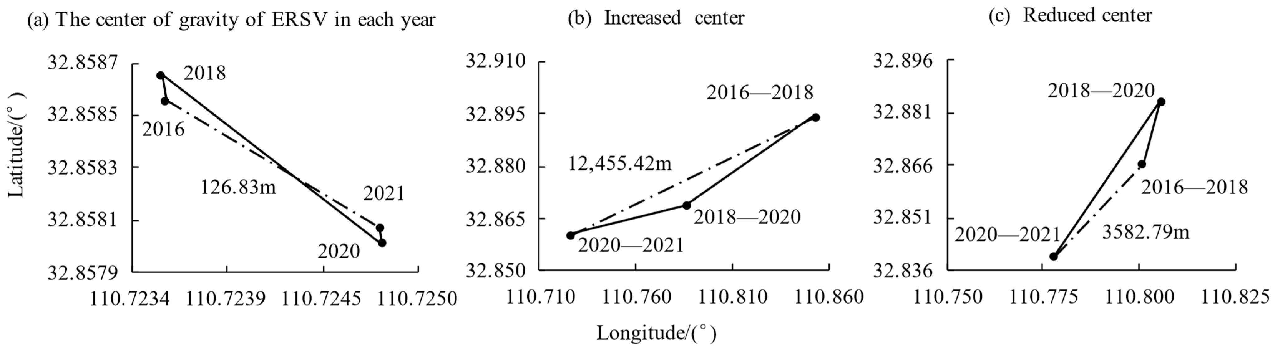
3.1.2. Spatial Dimension Analysis of ERSV

Based on the ERSV data collected from ecological plots in Yunyang District of Hubei Province from 2016 to 2021, the unit ERSV and ERSV change rates for each plot were calculated (Figure 3). The results revealed significant spatial differentiation in ERSVs, with high values in the north and south and low values in the middle. The areas with high ERSVs were primarily woodland plots, such as Baoxia Town, Canglangshan Forest Farm, Yeda Township in the southwest, and Daliu Township in the north, as well as the wetland distribution area of Yunyang District. These areas had higher unit ERSV values. In contrast, the areas with low ERSVs were mainly located in Chengguan Town, Chadian Town, Liupi Town in the central region, and Meipu Town in the northeast, which are urban areas with high levels of human activity. These areas had lower unit ERSV values. These findings are consistent with previous studies by Zheng et al. [31] and Li et al. [30], which also reported a high and low spatial distribution of the ESV in Hubei Province based on different grid scales. The ERSV changes in each ecological plot in Yunyang District during 2018–2020 reflect the overall trend of ERSV variation from 2016 to 2021. Overall, the ERSVs of all ecological plots showed an increase, with the most significant increase observed in wetland ecosystems, indicating the success of wetland restoration efforts in Yunyang District of Hubei Province.

Based on the ERSV data from ecological plots in Yunyang District of Hubei Province and their changes from 2016 to 2021, the spatiotemporal information of ERSV and its shifting center of gravity were obtained using the ArcGIS10.8 center of gravity model (Figure 4). The analysis revealed that the center of gravity of ERSV shifted in a northwestern direction, then to the southeast, and finally back to the northwest. The overall shift was 126.83 m to the southeast, with small and consistent shifts in each year. This suggests that the spatial pattern of ERSV in Yunyang District, Hubei Province remained relatively stable. The center of gravity of ERSV increased and continued to shift to the southwest, with an overall shift of 12,455.42 m. This was greater than the shift of the center of gravity of ERSV reduction, which first shifted to the northeast and then to the southwest, with an overall shift of 3582.79 m to the southwest. These findings confirm that the ERSV in Yunyang District, Hubei Province mainly increased from 2016 to 2021 and that the ecosystem recovery in the southwest area was relatively better than in other areas.

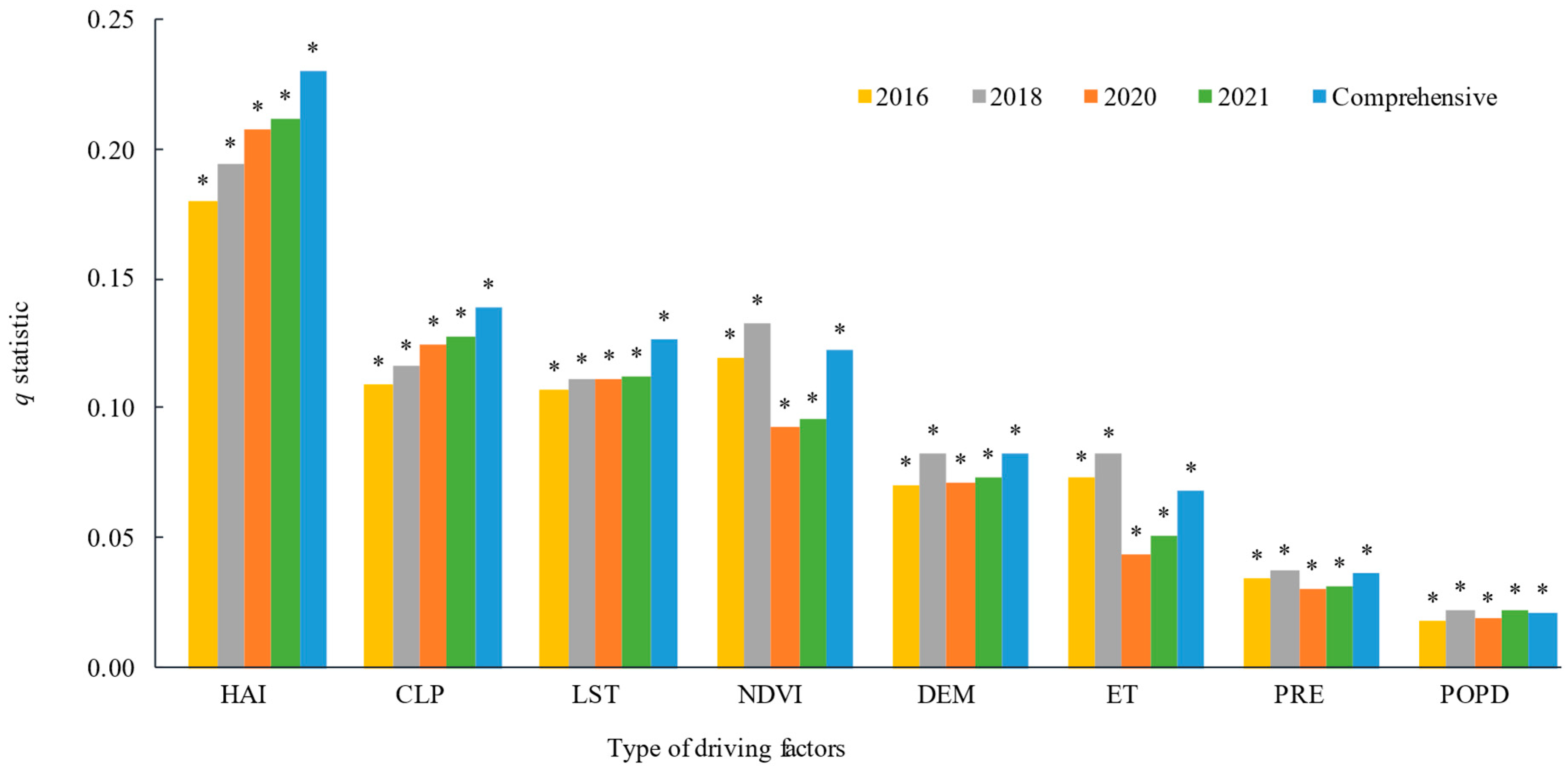
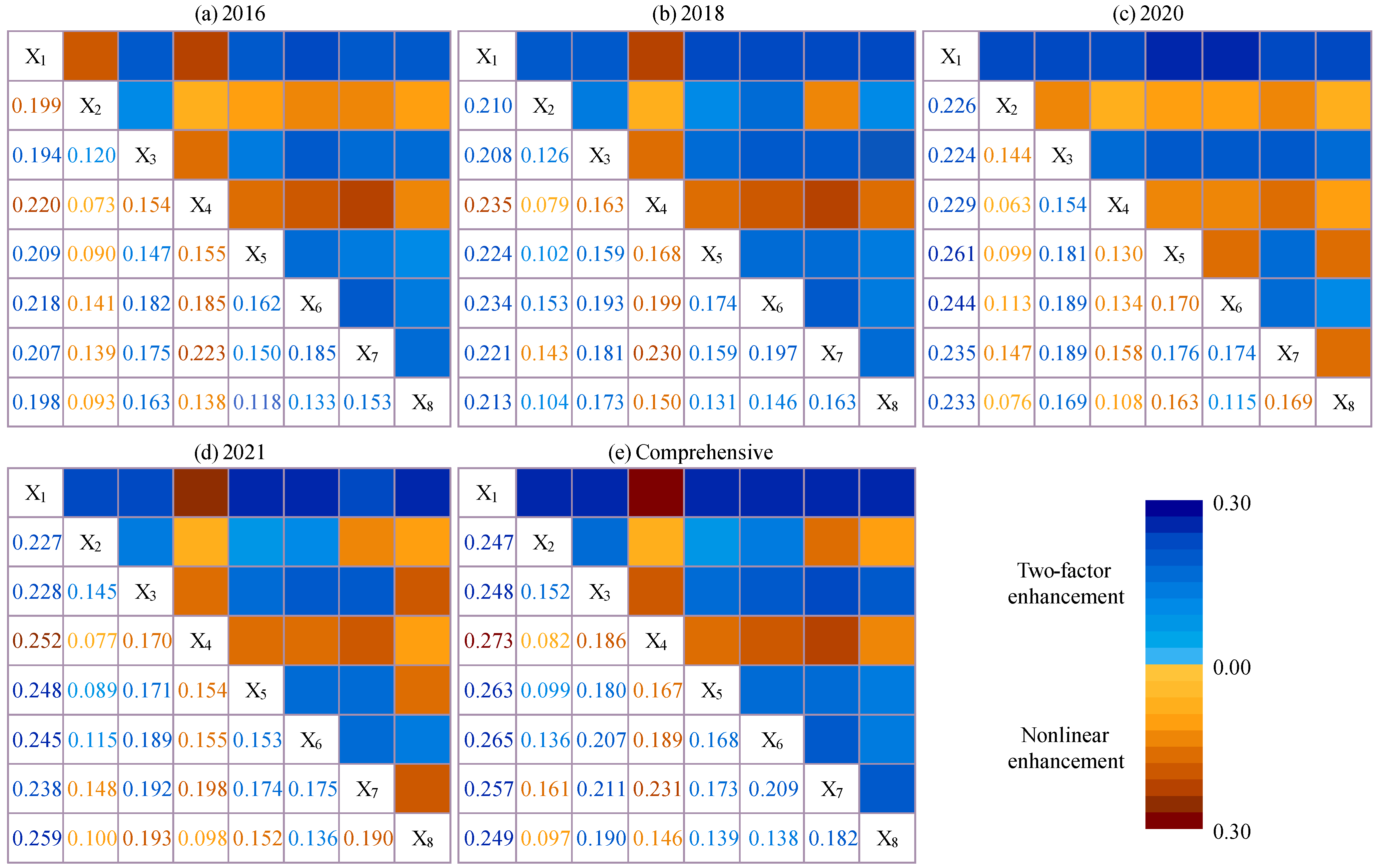
3.2. Analysis of Driving Factors for the Spatial Differentiation of ERSV

The OPGD’s factor detector and interaction detector were utilized to analyze the explanatory power of various factors (HAI, POPD, CLP, PRE, DEM, NDVI, LST, and ET) on the regional heterogeneity of the ERSV in Yunyang District of Hubei Province, as well as the interaction characteristics between each driving factor. By calculating the average values of each factor and the ERSV from 2016 to 2021, the OPGD was able to comprehensively analyze the influence of each factor.

The results of the single factor detection (Figure 5) showed that anthropogenic factors had greater explanatory power regarding the spatial differentiation of the ERSV in Yunyang District compared to natural factors (p < 0.01). HAI was the dominant anthropogenic factor, with a q statistic of 0.230 for the comprehensive explanatory power of the ERSV, followed by CLP, with a q statistic of 0.139. LST and NDVI were the main natural factors, with comprehensive explanatory power q statistics of 0.127 and 0.122, respectively. The explanatory power of other factors was less than 0.100. In terms of the temporal dimension, it was observed that the explanatory power of HAI, CLP, and LST on the regional heterogeneity of the ERSV increased year by year, while the other factors showed varying degrees of increase, decrease, and fluctuation.

The interaction results of various factors (Figure 6) revealed that the explanatory power of the interaction between any two driving factors regarding the spatial differentiation of the ERSV in Yunyang District was greater than that of a single factor, and both showed nonlinear enhancement or two-factor enhancement characteristics. This suggests that the combined effect of different factors can enhance the explanatory power of ERSV [41]. The interaction between HAI and other factors had the most significant enhancement effect, with the interaction between HAI and natural factors being stronger than that between HAI and anthropogenic factors. Among these, the interaction between HAI and PRE was the strongest and showed two-factor enhancement characteristics, with a comprehensive explanatory power of 27.3%. This indicates that the interaction between these two factors plays a crucial role in the spatial differentiation of ERSV. Overall, the interaction between HAI and natural factors, as well as LST and anthropogenic factors, greatly enhances the explanatory power of the spatial differentiation of ERSV in Yunyang District, highlighting the strong coupling effect of anthropogenic and natural factors in promoting regional ERSV.

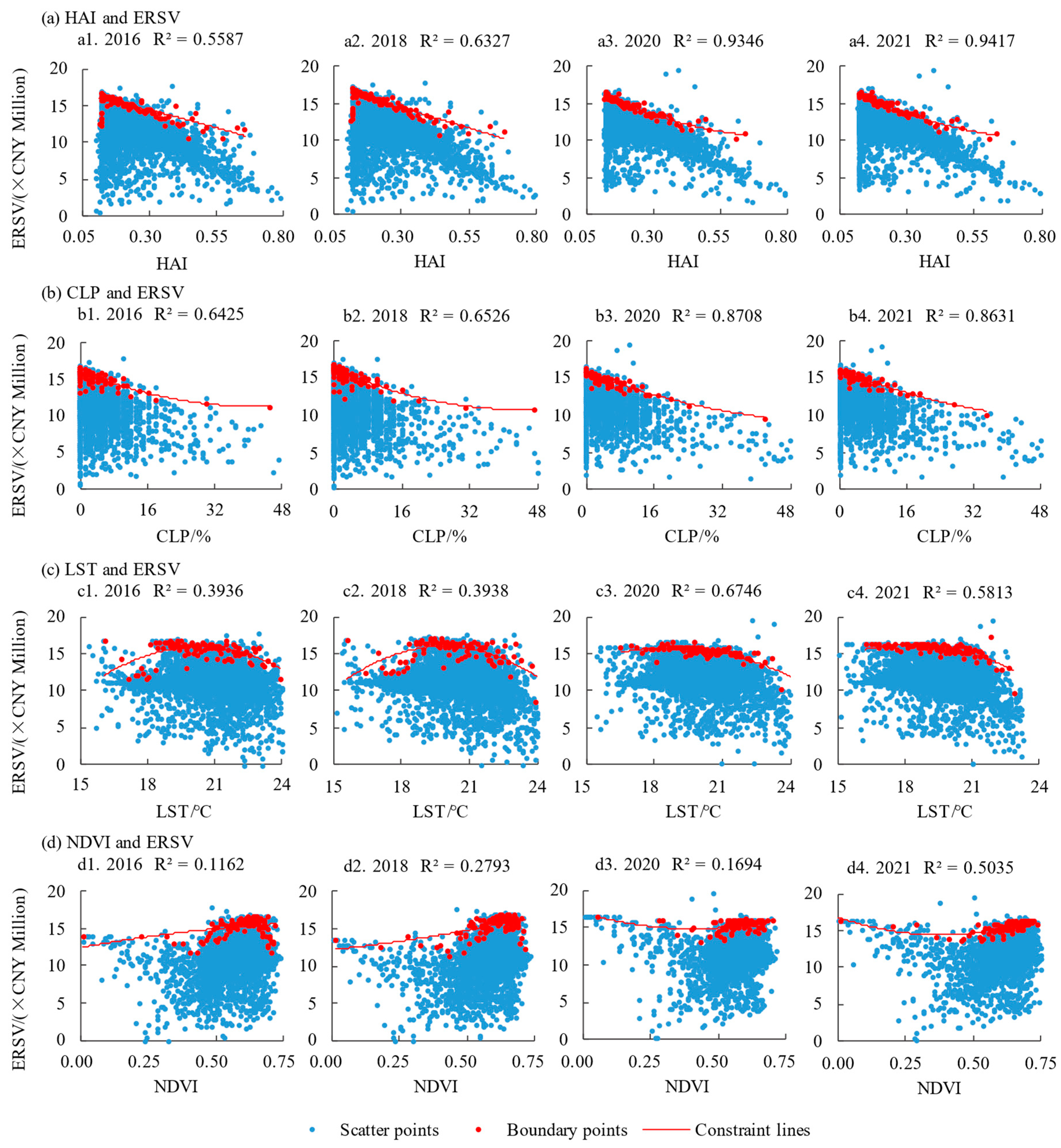
3.3. Analysis of the Constraint Relationship between the Major Driving Factors and ERSV

In the Yunyang District of Hubei Province, four driving factors (HAI, CLP, LST, and NDVI) were identified as having the strongest explanatory power for the spatial differentiation of ERSV through factor detection analysis. The constraint relationship between these factors and ERSV was then analyzed using the constraint line extraction method in order to reveal the influence mechanism of major anthropogenic and natural factors regarding the qualitative constraint of ERSV.

The results of the constraint line extraction showed an inverse proportional constraint between major anthropogenic factors (HAI, CLP) and ERSV (Figure 7a,b) from 2016 to 2021, and this had a significant negative inhibitory effect on ERSV. This suggests that human activities have a direct impact on the decline in ERSV [16], and an increase in human activity intensity weakens ecological stability. Only when HAI is less than 0.3 and CLP is less than 16% can ERSV maintain a high and stable level.

The constraint line between major natural factors (LST) and ERSV in Yunyang District of Hubei Province follows a hump-shaped pattern (Figure 7c), with ERSV increasing and then decreasing as LST increases, and the constraint effect follows a similar trend, which had a negative inhibitory effect on ERSV on the whole. The optimal area for ERSV production is when LST is between 18 and 22 °C. As a whole, NDVI had a positive effect on ERSV, and over time, the constraint relationship between NDVI and ERSV has shifted from an inverse tangent constraint to a “U” constraint (Figure 7d), indicating that the ecological recovery of low-NDVI regions in Yunyang District is good. However, it should be noted that these regions have a weak constraint effect on ERSV, and only when NDVI is greater than 0.5 is the constraint effect on ERSV the most stable. This suggests that low-NDVI regions are ecologically fragile and have relatively weak internal stability.

4. Discussion

4.1. Calculation and Spatiotemporal Characteristics of ERSV at the Plot Scale

The calculation and analysis of ERSV at different scales was conducted using panel data from administrative divisions and land use raster data [20,21,23,26]; the results of the ERSV calculation at the plot scale in Yunyang District provided more detailed information on the spatial distribution, allowing for a better understanding of the regional spatial differentiation of ERSV. This was achieved by resampling the grid parameters and spatializing the statistical data, which unified the multi-source data into plot units. This approach allowed for the calculation of the ERSV for each plot, providing a finer grasp of the regional ERSV. Additionally, the analysis of the plot scale ERSV revealed similar spatiotemporal characteristics as previous studies based on grid scale ERSV, including the trend of decreasing and then increasing ERSV in Yunyang District from 2016 to 2020 [31,43] and the distribution characteristics of high- and low-ERSV regions [30,31]. This further supports the scientific validity of this study.

4.2. Driving Factors of ERSV at the Plot Scale

In this study, nine indicators were selected to examine the potential impact on the spatial differentiation of ERSV in Yunyang District. Unlike previous studies that solely utilized the natural breakpoint method [44,45] for data discretization, this study employed the OPGD method to optimize the process [38,39]. Taking the discretization process of each driver factor datum of ERSV in Yunyang District in 2020 as an example, the optimal parameters of the OPGD model were tested, and according to the parameter combination with the largest q value, the optimal classification method and the number of classification categories for the discretization process of each driving factor were determined. As shown in Figure 8, the HAI was divided into five categories using the quantile method. The PRE and NDVI were divided into eight categories, while the POPD was divided into six categories using the natural breakpoint method. The CLP and LST were divided into six categories using the geometric interval method. The DEM and ET were divided into eight categories using the standard deviation method. This resulted in the optimal discretization process for each driving factor datum. The same process was applied to the remaining years, taking into consideration the optimal parameters determined for the 2020 OPGD model.

Based on the results of the OPGD model, the optimal parameter combination has been selected for a more accurate analysis of drivers. The findings indicate that HAI, CLP, LST, and NDVI are the dominant factors influencing the spatial differentiation of ERSV in Yunyang District. HAI, CLP, and LST have a negative inhibitory effect on ERSV, while NDVI has a positive promoting effect. The ERSV maintains a high and stable value output when the HAI is less than 0.3, CLP is less than 15%, LST is between 18 and 22 °C, and NDVI is greater than 0.5. However, the interaction between HAI and PRE has the greatest influence on the spatial differentiation of ERSV, even though drivers such as PRE have little direct impact on ERSV. The impact of multiple factors on the ERSV in Yunyang District is not simply the sum of individual factors but rather the result of their integrated influence. Therefore, in order to improve the regional ERSV, it is necessary to consider a variety of driving factors and pay attention to the interaction between HAI and PRE. In regional management, differentiated, diversified, and precise regulation strategies should be implemented to maintain the efficiency and stability of the ERSV output.

4.3. Uncertainty Analysis and Prospect

(1)

The accounting of ERSV involves multiple disciplines, resulting in the poor comparability of the results [22]. In this study, only nine ESs were selected to calculate ERSV, and the negative oxygen ion and noise reduction function values were not included, resulting in a low ERSV calculation result. In addition, the multi-source raster data were resampled to 5 m × 5 m in this study, allowing for the calculation and analysis of ERSV at the plot scale. However, the nature of the data was not considered, and no analysis or verification was conducted, potentially increasing the uncertainty of the results. In future studies, it would be beneficial to develop selection and accounting criteria for regional ecosystem service indicators based on the ecological background characteristics and project requirements of the study area. Additionally, appropriate interpolation methods and resolutions should be chosen through experimental verification to achieve a more accurate and comprehensive quantitative study of ERSV.

(2)

This paper examines the factors that drive ERSV and establishes a relationship between ERSV and major anthropogenic and natural drivers. However, in practical management, more attention is given to how these drivers impact the value of individual ecosystem service functions. Additionally, due to the limited access to continuous data on driving factors such as CO₂ emissions and GDP, they were not included in the analysis. This may affect the scientific validity of the research and its conclusions. In future studies, a more comprehensive and diverse range of driving factor indictors should be considered for the analysis. Furthermore, the spatial and temporal characteristics, as well as the driving factors and constraint line relationships of ecosystem service function values, should be integrated into management practices to inform more targeted and scientifically sound decision-making.

5. Conclusions

In this study, we analyzed the spatiotemporal evolution characteristics of the ERSV in Yunyang District of Hubei Province by constructing an ERSV accounting model at the plot scale. We used the OPGD and constraint line extraction method to identify the driving factors and constraint rules of ERSV. The primary conclusions are listed below.

(1)

In the temporal dimension, the ERSV in Yunyang District showed a small decrease at first and then a continuous increase from 2016 to 2021, with an overall increase of CNY 1.664 billion and a growth rate of 3.68%. The contribution values of the climate regulation function and water retention function to ERSV were significant.

(2)

In the spatial dimension, ERSV was distributed higher in the north and south and lower in the middle. The high-value areas were mainly located in woodland and wetland areas with high unit ERSVs. The center of gravity of the ERSV increase shifted to the southwest by 12,455.42 m, while the center of gravity of the reduction shifted to the southwest by 3582.79 m from 2016 to 2021.

(3)

The analysis of driving factors showed that the HAI and CLP were the leading anthropogenic factors, while the LST and NDVI were the leading natural factors. The interaction between any two factors showed nonlinear enhancement or two-factor enhancement characteristics, and the interaction between HAI and natural factors and LST and anthropogenic factors greatly enhanced the explanatory power regarding the spatial differentiation of ERSV.

(4)

The HAI, CLP, and LST all had a negative inhibitory effect on the ERSV, while the NDVI had a positive promoting effect overall. The ERSV was able to maintain a consistently high value output when the HAI was below 0.3, CLP was below 15%, LST was between 18 and 22 °C, and NDVI was greater than 0.5.

References

1. Daily, G.C. Nature’s Services: Societal Dependence on Natural Ecosystems; Island Press: Washington, DC, USA, 1997. [Google Scholar]
2. Ouyang, Z.; Wang, X.; Miao, H. A primary study on Chinese terrestrial ecosystem services and their ecological economic values. Acta Ecol. Sin. 1999, 19, 607–613. [Google Scholar]
3. Costanza, R.; d’Arge, R.; de Groot, R.; Farber, S.; Grasso, M.; Hannon, B.; Limburg, K.; Naeem, S.; O’Neill, R.V.; Paruelo, J.; et al. The value of the world’s ecosystem services and natural capital. Nature 1997, 387, 253–260. [Google Scholar] [CrossRef]
4. Fu, B.; Zhou, G.; Bai, Y.; Song, C.; Liu, J.; Zhang, H.; Lu, Y.; Zheng, H.; Xie, G. The Main Terrestrial Ecosystem Services and Ecological Security in China. Adv. Earth Sci. 2009, 24, 571–576. [Google Scholar]
5. Ouyang, Z.Y.; Zheng, H.; Xiao, Y.; Polasky, S.; Liu, J.G.; Xu, W.H.; Wang, Q.; Zhang, L.; Xiao, Y.; Rao, E.M.; et al. Improvements in ecosystem services from investments in natural capital. Science 2016, 352, 1455–1459. [Google Scholar] [CrossRef]
6. Xie, G.; Zhang, C.; Zhang, C.; Xiao, Y.; Lu, C. The value of ecosystem services in China. Resour. Sci. 2015, 37, 1740–1746. [Google Scholar]
7. Ouyang, Z.; Song, C.; Zheng, H.; Polasky, S.; Xiao, Y.; Bateman, I.J.; Liu, J.; Ruckelshaus, M.; Shi, F.; Xiao, Y.; et al. Using gross ecosystem product (GEP) to value nature in decision making. Proc. Natl. Acad. Sci. USA 2020, 117, 14593–14601. [Google Scholar] [CrossRef]
8. Song, C.; Ouyang, Z. Gross Ecosystem Product accounting for ecological benefits assessment: A case study of Qinghai Province. Acta Ecol. Sin. 2020, 40, 3207–3217. [Google Scholar]
9. Ouyang, Z.; Zhu, C.; Yang, G.; Xu, W.; Zheng, H.; Zhang, Y.; Xiao, Y. Gross ecosystem product: Concept, accounting framework and case study. Acta Ecol. Sin. 2013, 33, 6747–6761. [Google Scholar] [CrossRef]
10. Wang, L.; Xiao, Y.; Ouyang, Z.; Wei, Q.; Bo, W.; Zhang, J.; Ren, L. Gross ecosystem product accounting in the national key ecological function area: An example of Arxan. China Popul. Resour. Environ. 2017, 27, 146–154. [Google Scholar]
11. Pema, D.; Xiao, Y.; Ouyang, Z.; Wang, L. Gross ecosystem product accounting for the Garze Tibetan Autonomous Prefecture. Acta Ecol. Sin. 2017, 37, 6302–6312. [Google Scholar]
12. Ma, G.; Yu, F.; Wang, J.; Zhou, X.; Yuan, J.; Mou, X.; Zhou, Y.; Yang, W.; Peng, F. Measuring gross ecosystem product (GEP) of 2015 for terrestrial ecosystems in China. China Environ. Sci. 2017, 37, 1474–1482. [Google Scholar]
13. Pema, D.; Xiao, Y.; Ouyang, Z.; Wang, L. Assessment of ecological conservation effect in Xishui county based on gross ecosystem product. Acta Ecol. Sin. 2020, 40, 499–509. [Google Scholar]
14. Liu, J.G.; Viña, A.; Yang, W.; Li, S.X.; Xu, W.H.; Zheng, H. China’s Environment on a Metacoupled Planet. In Annual Review of Environment and Resources; Gadgil, A., Tomich, T.P., Eds.; Annual Reviews, Palo Alto: Santa Clara, CA, USA, 2018; Volume 43, pp. 1–34. [Google Scholar]
15. Ouyang, Z.; Lin, Y.; Song, C. Research on Gross Ecosystem Product(GEP): Case study of Lishui City, Zhejiang Province. Environ. Sustain. Dev. 2020, 45, 80–85. [Google Scholar]
16. Millennium Ecosystem Assessment (MEA). Ecosystems and Human Well-Being: A Framework for Assessment; Island Press: Washington, DC, USA, 2005. [Google Scholar]
17. Li, F.Z.; Yin, X.X.; Shao, M. Natural and anthropogenic factors on China’s ecosystem services: Comparison and spillover effect perspective. J. Environ. Manag. 2022, 324, 9. [Google Scholar] [CrossRef] [PubMed]
18. Shen, J.S.; Li, S.C.; Wang, H.; Wu, S.Y.; Liang, Z.; Zhang, Y.T.; Wei, F.L.; Li, S.; Ma, L.; Wang, Y.Y.; et al. Understanding the spatial relationships and drivers of ecosystem service supply-demand mismatches towards spatially-targeted management of social-ecological system. J. Clean. Prod. 2023, 406, 14. [Google Scholar] [CrossRef]
19. Xu, X.B.; Yang, G.S.; Tan, Y. Identifying ecological red lines in China’s Yangtze River Economic Belt: A regional approach. Ecol. Indic. 2019, 96, 635–646. [Google Scholar] [CrossRef]
20. Yang, M.; Xiao, Y.; Ouyang, Z.; Ye, H.; Deng, M.; Ai, L. Ecosystem regulation services accounting of gross ecosystem product (GEP) in Sichuan province. J. Southwest Minzu Univ. 2019, 45, 221–232. [Google Scholar]
21. Chen, M.; Ji, R.; Liu, X.; Liu, C.; Su, L.; Zhang, L. Gross ecosystem product accounting for Two Mountains’ Bases and transformation analysis: The case study of Ninghai County. Acta Ecol. Sin. 2021, 41, 5899–5907. [Google Scholar]
22. Mou, X.; Wang, X.; Zhang, X.; Rao, S.; Zhu, Z. Accounting and Mapping of Gross Ecosystem Product in Yanqing District, Beijing. Res. Soil Water Conserv. 2020, 27, 265–274+282. [Google Scholar]
23. Chen, H.; Wang, Y.; Huang, Y.; Wu, B.; Lai, W. Evaluation of Regional Ecosystem Services Grade Coupling Ecological Carrying Capacity and Gross Ecosystem Product—A Case Study of Changting County, Fujian Province. J. Soil Water Conserv. 2021, 35, 150–160. [Google Scholar]
24. Hu, C.; Zou, B.; Liang, Y.; He, C.; Lin, Z. Spatio-temporal evolution of gross ecosystem product with high spatial resolution: A case study of Hunan Province during 2000–2020. Remote Sens. Nat. Resour. 2023, 35, 179–189. [Google Scholar]
25. Jiang, S. Gross Ecosystem Product Accounting with its Spatio-Temporal Evolution of Shaanxi Province; Northwest A&F University: Xianyang, China, 2021. [Google Scholar]
26. Yu, M.; Jin, H.; Li, Q.; Yao, Y.; Zhang, Z. Gross Ecosystem Product (GEP) Accounting for Chenggong District. J. West China For. Sci. 2020, 49, 41–48+55. [Google Scholar]
27. Hao, C.; Wu, S.; Zhang, W.; Chen, Y.; Ren, Y.; Chen, X.; Wang, H.; Zhang, L. A critical review of Gross ecosystem product accounting in China: Status quo, problems and future directions. J. Environ. Manag. 2022, 322, 14. [Google Scholar] [CrossRef]
28. Wang, Y.; Ding, J.; Li, X.; Zhang, J.; Ma, G. Impact of LUCC on ecosystem services values in the Yili River Basin based on an intensity analysis model. Acta Ecol. Sin. 2022, 42, 3106–3118. [Google Scholar]
29. Zeng, C.; Li, Y.; Duan, X.; Xu, Y. Assessment and Driving Force Analysis of Ecosystem Service Value in the Urban Agglomeration Along the Middle Reaches of the Yangtze River. Res. Soil Water Conserv. 2022, 29, 362–371. [Google Scholar]
30. Li, Z.; Chen, J.; Zhang, W.; Lei, L.; Sha, Z. Analysis of evolution and influencing factors of ecosystem service value in Hubei Province. Sci. Surv. Mapp. 2023, 48, 245–257. [Google Scholar]
31. Zheng, X.; Chen, Y.; Zheng, Z.; Guo, C.; Huang, Z.; Zhou, Y. Dynamic Changes of Ecosystem Service Value and Evolution of Its Influencing Factors in Hubei Province. Ecol. Environ. Sci. 2023, 32, 195–206. [Google Scholar]
32. Yan, E.; Lin, H.; Wang, G.; Xia, C. Analysis of evolution and driving force of ecosystem service values in the Three Gorges Reservoir region during 1990–2011. Acta Ecol. Sin. 2014, 34, 5962–5973. [Google Scholar]
33. Chinese Academy of Environmental Planning, Research Center for Eco-Environmental Sciences. The Technical Guideline on Gross Ecosystem Product (GEP). 2020. Available online: https://www.caep.org.cn/zclm/sthjyjjhszx/zxdt_21932/202010/W020201029488841168291.pdf (accessed on 16 July 2023).
34. National Development and Reform Commission of China, National Bureau of Statistics of China. The Code for Gross Ecological Product Accounting; People’s Publishing House: Beijing, China, 2022. [Google Scholar]
35. Fu, J.; Zhang, Q.; Wang, P.; Zhang, L.; Tian, Y.; Li, X. Spatio-Temporal Changes in Ecosystem Service Value and Its Coordinated Development with Economy: A Case Study in Hainan Province, China. Remote Sens. 2022, 14, 970. [Google Scholar] [CrossRef]
36. Yuan, H.; Yan, J.; Zhang, J.; Wang, Z.; Xu, W.; Zhang, H. Influences of climate change and human activities on vegetation phenology of Shanghai. Acta Ecol. Sin. 2023, 43, 8803–8815. [Google Scholar]
37. Wang, J.; Xu, C. Geodetector: Principle and prospective. Acta Geogr. Sin. 2017, 72, 116–134. [Google Scholar]
38. Song, Y.Z.; Wang, J.F.; Ge, Y.; Xu, C.D. An optimal parameters-based geographical detector model enhances geographic characteristics of explanatory variables for spatial heterogeneity analysis: Cases with different types of spatial data. Giscience Remote Sens. 2020, 57, 593–610. [Google Scholar] [CrossRef]
39. Li, Y.; Geng, H.C. Spatiotemporal trends in ecosystem carbon stock evolution and quantitative attribution in a karst watershed in southwest China. Ecol. Indic. 2023, 153, 13. [Google Scholar] [CrossRef]
40. Hao, R.; Yu, D.; Wu, J.; Guo, Q.; Liu, Y. Constraint line methods and the applications in ecology. Chin. J. Plant Ecol. 2016, 40, 1100–1109. [Google Scholar]
41. Fang, L.; Xu, D.; Wang, L.; Niu, Z.; Zhang, M. The study of ecosystem services and the comparison of trade-off and synergy in Yangtze River Basin and Yellow River Basin. Geogr. Res. 2021, 40, 821–838. [Google Scholar]
42. Li, D.L.; Cao, W.F.; Dou, Y.H.; Wu, S.Y.; Liu, J.G.; Li, S.C. Non-linear effects of natural and anthropogenic drivers on ecosystem services: Integrating thresholds into conservation planning. J. Environ. Manag. 2022, 321, 11. [Google Scholar] [CrossRef] [PubMed]
43. Jiu, J. Study on the Implication of Land Use Change on Ecosystem Service Value in Hubei Province; Huazhong University of Science and Technology: Wuhan, China, 2021. [Google Scholar]
44. He, Y.; Sheng, M.; Lei, L.; Guo, K.; He, Z. Driving factors and spatio-temporal distribution on NO2 and CO2 in the Yangtze River Delta. China Environ. Sci 2020, 42, 3544–3553. [Google Scholar]
45. Wang, R.; Zhang, H.; Qiang, W.; Li, F.; Peng, J. Spatial characteristics and influencing factors of carbon emissions in county-level cities of China based on urbanization. Prog. Geogr. 2021, 40, 1999–2010. [Google Scholar] [CrossRef]
Figure 1. Location of the study area.
Sustainability 16 04548 g001
Figure 2. Comparison of ecological plots before and after refinement in 2021: (a) Original; (b) After refinement.
Sustainability 16 04548 g002
Figure 3. Ecosystem regulation services value (ERSV), unit ERSV, and ERSV change rate of each plot in Yunyang District of Hubei Province from 2016 to 2021: (a) ERSV of plots in 2016; (b) ERSV of plots in 2018; (c) ERSV of plots in 2020; (d) ERSV of plots in 2021; (e) unit ERSV of plots in 2016; (f) unit ERSV of plots in 2018; (g) unit ERSV of plots in 2020; (h) unit ERSV of plots in 2021; (i) ERSV change rate of plots from 2016 to 2018; (j) ERSV change rate of plots from 2018 to 2020; (k) ERSV change rate of plots from 2020 to 2021; (l) ERSV change rate of plots from 2016 to 2021.
Sustainability 16 04548 g003
Figure 4. Change in the center of gravity of the ERSV in Yunyang District of Hubei Province from 2016 to 2021: (a) The center of gravity of ERSV in each year; (b) Increased center; (c) Reduced center.
Sustainability 16 04548 g004
Figure 5. Results of the detection of driving factors. Note: HAI, human active index; POPD, population density; CLP, construction land proportion; PRE, annual precipitation; DEM, digital elevation model; NDVI, average annual normalized difference vegetation index; LST, average annual land surface temperature; ET, annual evapotranspiration. * denotes 1% significance levels.
Sustainability 16 04548 g005
Figure 6. Interaction results of various factors: (a) 2016; (b) 2018; (c) 2020; (d) 2021; (e) Comprehensive. Note: X1, HAI; X2, POPD; X3, CLP; X4, PRE; X5, DEM; X6, NDVI; X7, LST; X8, ET.
Sustainability 16 04548 g006
Figure 7. Scatter plots and constraint lines between major driving factors and ERSV: (a) HAI and ERSV; (b) CLP and ERSV; (c) LST and ERSV; (d) NDVI and ERSV.
Sustainability 16 04548 g007
Figure 8. Test results of the optimal parameters of each driving factor in 2020: (a) HAI; (b) POPD; (c) CLP; (d) PRE; (e) DEM; (f) NDVI; (g) LST; (h) ET.
Sustainability 16 04548 g008