Short-Term Traffic Flow Forecasting Method Based on Secondary Decomposition and Conventional Neural Network–Transformer

Abstract

Because of the random volatility of traffic data, short-term traffic flow forecasting has always been a problem that needs to be further researched. We developed a short-term traffic flow forecasting approach by applying a secondary decomposition strategy and CNN–Transformer model. Firstly, traffic flow data are decomposed by using a Complete Ensemble Empirical Mode Decomposition with Adaptive Noise (CEEMDAN) algorithm, and a series of intrinsic mode functions (IMFs) are obtained. Secondly, the IMF1 obtained from the CEEMDAN is further decomposed into some sub-series by using Variational Mode Decomposition (VMD) algorithm. Thirdly, the CNN–Transformer model is established for each IMF separately. The CNN model is employed to extract local spatial features, and then the Transformer model utilizes these features for global modeling and long-term relationship modeling. Finally, we obtain the final results by superimposing the forecasting results of each IMF component. The measured traffic flow dataset of urban expressways was used for experimental verification. The experimental results reveal the following: (1) The forecasting performance achieves remarkable improvement when considering secondary decomposition. Compared with the VMD-CNN–Transformer, the CEEMDAN-VMD-CNN–Transformer method declined by 25.84%, 23.15% and 22.38% in three-step-ahead forecasting in terms of MAPE. (2) It has been proven that our proposed CNN–Transformer model could achieve more outstanding forecasting performance. Compared with the CEEMDAN-VMD-CNN, the CEEMDAN-VMD-CNN–Transformer method declined by 13.58%, 11.88% and 11.10% in three-step-ahead forecasting in terms of MAPE.

1. Introduction

Timely and accurate traffic flow forecasting information could dynamically monitor the change trends of traffic conditions, and could predict road traffic demand and potential capacity. For travelers, it would enable them to change their travel route in a timely manner [1]. For traffic managers, precise traffic flow forecasting results are beneficial for making scientific and reasonable management and control decisions. However, short-term traffic flow data usually refers to data collected within 15 min. Because the time interval for data collection is small, short-term traffic flow data possess randomness and volatility. Therefore, short-term traffic flow forecasting is still challenging work, which requires a lot of effort to research.

Currently, numerous short-term traffic flow forecasting achievements have been put forward. These existing achievements can be mainly divided into two major kinds: statistical methods and machine learning methods. A conventional statistical method is to construct a specific mathematical model to reveal the distribution pattern of data. For example, Zhang [2] applied three statistical models to predict traffic data. The spectral analysis technique was used to predict periodic trends, the deterministic part was predicted using the ARIMA model, and the volatility part was predicted using the GJR-GARCH model. Lin [3] put forward traffic flow forecasting method by using the ARIMA model and GARCH model. Li [4] used a multiple linear regression model for short-term traffic flow forecasting. Zhou [5] employed a dual Kalman filtering model for forecasting short-term traffic flow data. The advantage of statistical methods lies in their simple structure and real-time correction of local trends in data. However, when fitting nonlinear data, the performance of this method will be greatly limited. To overcome these shortcomings, machine learning models are extensively employed for short-term traffic flow forecasting considering their excellent nonlinear fitting ability. For example, Xu et al. [6] predicted short-term traffic flow data by applying nonlinear autoregressive neural network model. Peng [7] combined wavelet denoising and a BPNN model for traffic flow prediction. Ma [8] employed an artificial neural network (ANN) model for forecasting traffic flow data, and the model was optimized by a genetic algorithm and exponential smoothing. Xu [9] applied a wavelet neural network (WNN) for short-term traffic flow forecasting, and the WNN model was optimized by a mind evolutionary algorithm. Feng [10] combined an adaptive multi-kernel SVM and spatial–temporal information for traffic flow prediction. Toan [11] applied an SVM model for short-term traffic flow forecasting. Yang [12] predicted short-term traffic flow data by using an Extreme Learning Machine (ELM) algorithm. Among the various machine learning models mentioned above, ANN models have the advantage of strong robustness. However, the selection of network parameters is a challenging task and model training generally takes too long. Compared with artificial neural network models, SVM has greatly improved its generalization ability and overcome some shortcomings of neural network models. However, its calculative complexity rises by a wide margin with an increase in sample size. Due to its fast computing and strong generalization ability, ELMs are popularly used for traffic flow forecasting, but their predictive performance is subject to input weights and biases.

In recent years, in the wake of the introduction of big data into intelligent transportation, data-driven methods are receiving more and more attention. Big data has provided unprecedented conditions for traffic flow forecasting, while also placing higher demands for traffic flow prediction modeling. Driven by massive traffic flow data, a key issue is how to fully explore the valuable information. Therefore, the idea of “data decomposition” is popularly applied to deal with the challenges of traffic flow forecasting. Another, more decisive issue is how to choose the appropriate forecasting model under the conditions of big data. Along with research gradually becoming in-depth, deep learning models are considered as excellent means of forecasting. Not only that, but previous studies have also shown that hybrid deep learning frameworks outperform individual deep learning models.

Inspired by existing research findings, we developed a short-term traffic flow forecasting approach by applying a secondary decomposition strategy and a CNN–Transformer model. The main contributions include the following aspects: (1) Traffic flow time series data are firstly decomposed by using the CEEMDAN algorithm, and a series of IMFs are obtained. (2) The highest-frequency sub-component IMF1 obtained from CEEMDAN is further decomposed by applying the VMD algorithm. (3) CNN–Transformer models are established for each sub-component obtained from CEEMDAN-VMD separately, and the final results are obtained by superimposing each sub-component’s forecasting results. (4) Experimental verification is conducted by applying the measured traffic flow data.

The remaining content is arranged as follows: Section 2 provides a review of the relevant literature. Section 3 indicates the theoretical backgrounds of the CEEMDAN algorithm, the VMD algorithm and the CNN–Transformer model, and provides the overall architecture of the proposed method. Section 4 conducts an experimental validation using the measured traffic flow data. The comparison and discussions are described in Section 5. Finally, some conclusions are reached in Section 6.

2. Literature Review

Short-term traffic flow forecasting is not an easy task because of its high volatility, nonlinearity and randomness. A lot of scholars have explored this high volatility and designed effective short-term traffic flow forecasting methods. This section provides a literature review on two aspects: data decomposition and deep learning models.

2.1. Data Decomposition

Short-term traffic flow data display typical volatility, making it difficult to achieve ideal results by constructing a direct forecasting model. Several existing studies have proven that “data decomposition” strategies are an excellent means to improve forecasting performance. For example, Bing et al. [13] combined VMD and an LSTM model for short-term traffic flow prediction. Huang [14] applied EMD and a Hilbert transform model for short-term traffic flow forecasting. Chen [15] employed both the EEMD algorithm and artificial neural network for traffic flow forecasting. Zheng [16] applied a graph convolutional network and wavelet algorithm to predict traffic flow data. Wu [17] utilized both the CEEMDAN algorithm and different machine learning models to forecast short-term traffic data. Yang [18] utilized improved VMD and an Extreme Learning Machine (ELM) model for traffic flow prediction. However, there are still many shortcomings in these methods. For example, the highest-frequency intrinsic mode function components obtained from various decomposition algorithms include generous noise signals, which may influence the forecasting effect. Most studies directly remove the highest-frequency component IMF1, but the useful information contained in IMF1 may also be deleted concurrently. So as to address these drawbacks, a secondary decomposition strategy is proposed. The method of secondary decomposition involves the highest-frequency part IMF1 obtained from the decomposition algorithm being further decomposed, while the useful information implied in IMF1 is preserved. Liu et al. [19] applied secondary decomposition and Elman neural networks to predict wind speed. Yin et al. [20] applied a CNN-LSTM model and secondary decomposition for wind power prediction. Sun et al. [21] combined a secondary decomposition strategy and an optimized BPNN model for wind speed forecasting. Wen [22] applied an improved secondary decomposition and optimized VMD for short-term load forecasting. Zhang [23] combined an adaptive secondary decomposition algorithm and a robust temporal convolutional network for short-term wind speed prediction. Zhao et al. [24] applied a secondary decomposition technique and an ELM model for short-term traffic flow prediction. Hu [25] combined denoising schemes and an echo state network for short-term traffic flow forecasting. Li et al. [26] decomposed the carbon price time series data using CEEMD and VMD, and BPNN was used to build forecasting models. Li et al. [27] applied improved CEEMDAN and the discrete wavelet transform to decompose the carbon price time series, and support vector regression and multi-layer perceptron were used to predict subsequences.

Since previous studies have shown the superiority of secondary decomposition, the selection of appropriate decomposition algorithms is crucial. Among the various data decomposition algorithms, CEEMDAN and VMD two excellent decomposition algorithms. CEEMDAN is an extended form of EMD. CEEMDAN enhances decomposition stability by introducing adaptive noise during the decomposition process. The CEEMDAN algorithm decomposes signal into several IMFs and a residual sequence. Each IMF represents the signal change on a specific frequency and time scale. Compared with traditional EMD and CEEMD, CEEMDAN has higher decomposition accuracy and stability, and is better at handling nonlinear temporal data. The VMD algorithm can solve endpoint effects and modal aliasing. VMD has the ability to alleviate the non-stationary nature of time series data. VMD does not require sliding window technology and is not affected by the selection of basic functions. Compared with other time-frequency analysis algorithms, it has a wider range of adaptability. Hence, this paper will employ both the CEEMDAN algorithm and the VMD algorithm to accomplish traffic flow data decomposition.

2.2. Deep Learning Forecasting Models

In terms of selecting forecasting models, various deep learning models are increasingly being employed by scholars. Do [28] developed a deep learning method that comprehensively considered the spatiotemporal correlation of traffic data. Zhang [29] applied a CNN algorithm to complete short-term traffic flow forecasting. Ma [30] designed a new approach for daily traffic flow prediction by using a CNN-LSTM model. Chen et al. [31] applied a dynamic graph convolutional network model to forecast traffic flow data. Bharti [32] employed Particle Swarm Optimization (PSO) and Bidirectional Long–Short-Term Memory (Bi-LSTM) for short-term traffic flow prediction. Shu [33] developed a traffic flow prediction method by using an improved Gate Recurrent Unit (GRU) model. Liu [34] proposed an autoencoder-based traffic flow prediction method. Sun [35] predicted traffic flow data by applying a temporal graph convolution network. Liu [36] implemented traffic flow prediction by applying a spatial–temporal graph convolution model that considered fundamental traffic diagram information. Wen et al. [37] implemented short-term traffic flow prediction by applying a Transformer model.

Among the various deep learning models, CNNs perform well when extracting spatial local correlation features from data, but faces challenges when monitoring long-term dependencies for temporal data, while Transformer can handle temporal data with long-term dependencies, but cannot extract spatial correlations from the data. There is a long-term time dependency between current traffic flow data and historical data. Not only that, but traffic data also exhibit significant spatial correlation. Therefore, the advantages of CNNs and Transformer can be comprehensively utilized to simultaneously obtain spatiotemporal characteristics.

Table 1. Summary of existing prediction methods.

Reference	Decomposition Algorithm	Forecasting Model	Forecasting Target
[19]	WPD + FEEMD	Elman	Wind speed
[20]	EMD + VMD	CNN-LSTM	Wind power
[21]	VMD + SGMD	BPNN	Wind speed
[22]	CEEMDAN + VMD	LSTM	Load
[23]	CEEMDAN + VMD	CNN	Wind speed
[24]	EMD + LMD	ELM	Short-term traffic flow
[25]	CEEMDAN + WPD	ESN	Short-term traffic flow
[26]	CEEMD + VMD	BPNN	Carbon price
[27]	CEEMDAN + WTD	SVR	Carbon price
Our method	CEEMDAN + VMD	CNN–Transformer	Short-term traffic flow

gives a summary of the existing prediction methods based on secondary decomposition strategies and machine learning models.

From Table 1, it can be seen that methods combining secondary decomposition and machine learning have been applied in many fields. This paper draws on the idea of secondary decomposition from the existing literature, and puts forward a hybrid short-term traffic flow forecasting method that combines secondary decomposition and a deep learning model. In terms of selecting decomposition algorithms, CEEMDAN and VMD have been proven to be very effective decomposition algorithms which are increasingly popular among scholars. The CEEMDAN algorithm can enhance decomposition stability, and the VMD algorithm can solve endpoint effects and modal aliasing. Hence, we selected the CEEMDAN algorithm and VMD algorithm separately to achieve the secondary decomposition of short-term traffic flow data. In terms of selecting deep learning models, most existing studies adopt a single deep learning model. Deep learning models are highly dependent on sample data, while single models may encounter some challenges in the process of handling high-complexity data. Therefore, hybrid deep learning models have received increasing attention from scholars. CNNs are adept at capturing the local features of sequences, while the Transformer model can capture global dependencies between timesteps. In this paper, we comprehensively utilize the advantages of CNNs and the Transformer model to implement short-term traffic flow prediction modeling.

3. Methodology

3.1. CEEMDAN Algorithm

EMD is an effective approach for processing non-stationary signals which decomposes complex original sequences into IMF components based on the fluctuation scale. However, to address the phenomenon of mode aliasing that occurs in the EMD process, Wu [38] incorporated white noise and presented the EEMD method. However, the residual white noise after decomposition resulted in poor completeness of the EEMD method. Torres et al. [39] proposed the CEEMDAN method, which adds adaptive Gaussian white noise, effectively solving mode aliasing and residual noise in the reconstructed sequence. This method has good decomposition completeness. The CEEMDAN method includes the following steps.

Step 1: Considering the original data s(t), a white noise signal is added to construct a new time series $s\left(t\right)+a_0{n}^i\left(t\right)$, and then the first modal component $IM{F}_1^i\left(t\right)$ is acquired by performing EMD decomposition:

$$s\left(t\right)+a_0{n}^i\left(t\right)=IM{F}_1^i\left(t\right)+r_1^i\left(t\right), i=1,2,\cdots ,N$$

(1)

where $n^i\left(t\right)$ indicates the white noise signal, a₀ indicates the noise intensity and $r_1^i\left(t\right)$ indicates the residual. The final first modal component ${\overline{IMF}}_1\left(t\right)$ is acquired by averaging $IM{F}_1^i\left(t\right)$:

$${\overline{IMF}}_1\left(t\right)=\frac{1}{N}{\displaystyle \sum _{i=1}^{N}IM{F}_1^i}\left(t\right)$$

(2)

Step 2: The final first residual signal is acquired by the following formula:

$$r_1\left(t\right)=s\left(t\right)-{\overline{IMF}}_1\left(t\right)$$

(3)

Step 3: $r_1\left(t\right)$ is decomposed N times as below:

$$r_1\left(t\right)+a_1{E}_1\left(n^i\left(t\right)\right)=IM{F}_2^i\left(t\right)+r_2^i\left(t\right), i=1,2,\cdots ,N$$

(4)

where $E_1\left(n^1\left(t\right)\right)$ indicates the first sub-mode of $n^i\left(t\right)$, $IM{F}_2^i\left(t\right)$ denotes the second modal component and $r_1^i\left(t\right)$ is the residual. Therefore, the final ${\overline{IMF}}_2\left(t\right)$ is acquired by using the following formula:

$$\overline{IM{F}_2}\left(t\right)=\frac{1}{N}{\displaystyle \sum _{i=1}^{N}IM{F}_2^i}\left(t\right)$$

(5)

Step 4: The k-th residue is acquired according to the following formula:

$$r_k\left(t\right)=r_{k-1}\left(t\right)-{\overline{IMF}}_k\left(t\right)$$

(6)

Step 5: $r_k\left(t\right)$ is decomposed N times as follows:

$$r_k\left(t\right)+a_k{E}_k\left(n^i\left(t\right)\right)=IM{F}_{k+1}^i\left(t\right)+r_{k+1}^i\left(t\right), i=1,2,\cdots ,N$$

(7)

The final ${\overline{IMF}}_{k+1}\left(t\right)$ is acquired as follows:

$${\overline{IMF}}_{k+1}\left(t\right)=\frac{1}{N}{\displaystyle \sum _{i=1}^{N}IM{F}_{k+1}^i}\left(t\right)$$

(8)

Step 6: Step 4 and Step 5 are repeated, and the end condition for step execution is the amount of extreme points reached below 2. R(t) is obtained as follows:

$$R\left(t\right)=s\left(t\right)-{\displaystyle \sum _k{\overline{IMF}}_k\left(t\right)}$$

(9)

In summary, the original traffic flow data can be reconstructed as:

$$s\left(t\right)={\displaystyle \sum _k{\overline{IMF}}_k\left(t\right)}+R\left(t\right)$$

(10)

3.2. VMD Algorithm

VMD is a new time-frequency analysis algorithm proposed by Dragomiretskiy [40]. The IMF1 obtained from CEEMDAN is further decomposed into several sub-series by applying the VMD algorithm. The basic principle of VMD is that a time series signal is decomposed into multiple fixed-frequency-bandwidth modal components. Each modal component corresponds to a specific frequency and amplitude in the signal. These components are obtained by solving the optimization problem of minimizing a variational regularization function. Its advantage lies in its ability to adaptively decompose signals, without the need to know the frequency information in the signal beforehand. VMD gradually extracts the modal components of different frequencies from the signal through an iterative optimization solution process. In each iteration, the residual of the signal is updated based on the obtained modal components, and the search for the next frequency’s modal component continues until the stopping criterion is met.

The following formula expresses the constrained variational problem:

$${\min }_{u_k,w_k}\left\{{\displaystyle {\sum }_{k=1}^K{‖{\partial }_t\left[\left(\delta \left(t\right)+\frac{j}{\pi t}\right)\cdot u_k\left(t\right)\right]e^{-j{w}_{k}t}‖}_2^2}\right\}$$

$$s.t. {\displaystyle \sum _{k=1}^K{u}_k}=f\left(t\right)$$

(11)

where f(t) denotes a time series signal, u_k is the kth modal component obtained from the VMD, $\delta \left(t\right)$ is the Dirac function and w_k is the kth center frequency obtained from the VMD.

The Lagrangian multiplier $\lambda \left(t\right)$ and penalty factor $\alpha$ are employed to solve the above optimization problem:

$$L\left(u_k,w_k,\lambda \right)=\alpha {\displaystyle {\sum }_{k=1}^K{‖{\partial }_t\left[\left(\delta \left(t\right)+\frac{j}{\pi t}\right)\cdot u_k\left(t\right)\right]e^{-j{w}_{k}t}‖}_2^2}+{‖f\left(t\right)-{\displaystyle {\sum }_{k=1}^K{u}_k\left(t\right)}‖}_2^2+〈\lambda \left(t\right),f\left(t\right)-{\displaystyle {\sum }_{k=1}^K{u}_k\left(t\right)}〉$$

(12)

The alternating multiplication operator is employed to obtain the optimal solution for the constrained variational equation. The variable update formulas are as follows:

$${\widehat{u}}_k^{n+1}\left(w\right)=\frac{\widehat{f}\left(w\right)-{\displaystyle {\sum }_{i\ne j}{\widehat{u}}_i\left(w\right)+\frac{\widehat{\lambda }\left(w\right)}{2}}}{1+2\alpha {\left(w-w_k\right)}^2}$$

(13)

$$w_k^{n+1}=\frac{{\displaystyle {\int }_0^{\infty }w\left|{\widehat{u}}_k\left(w\right)\left|{ }^2\right.dw\right.}}{{\displaystyle {\int }_0^{\infty }\left|{\widehat{u}}_k\left(w\right)\left|{ }^2\right.dw\right.}}$$

(14)

$${\widehat{\lambda }}_k^{n+1}(\omega )={\widehat{\lambda }}^n(\omega )+r\left(\widehat{f}(\omega )-{\displaystyle \sum _{k+1}^n{\widehat{\mu }}_k^{n+1}(\omega )}\right)$$

(15)

where ${\widehat{\mu }}_k^{n+1}(\omega )$, $w_k^{n+1}(\omega )$ and ${\widehat{\lambda }}_k^{n+1}(\omega )$ are the updated values of ${\mu }_k$, ${\omega }_k$ and ${\lambda }_k$ obtained by Fourier transform.

The specific execution steps for VMD are as follows:

Step 1:$\left\{u_k^1\right\}$, $\left\{w_k^1\right\}$ and ${\lambda }^1$ are initialized. The iteration steps are set to 1.

Step 2: For each iteration step, ${\widehat{u}}_k^{n+1}\left(w\right)$ and $w_k^{n+1}$ are updated according to the Formulas (15) and (16).

Step 3: For $w\ge 0$, the ${\lambda }^n$ is updated by using Formula (16):

$${\lambda }^{n+1}\left(w\right)={\lambda }^n\left(w\right)+\tau \left(\widehat{u}\left(w\right)-{\displaystyle {\sum }_{k=1}^k{\widehat{u}}_k^{n+1}\left(w\right)}\right)$$

(16)

Step 4: Implement Step 2 and Step 3 repeatedly until the constraint condition is met; that is

$${\displaystyle {\sum }_k\frac{{‖{\widehat{u}}_k^{n+1}-{\widehat{u}}_k^n‖}_2^2}{{‖{\widehat{u}}_k^n‖}_2^2}}$$

(17)

3.3. The CNN–Transformer Forecasting Model

The CNN–Transformer model is applied for prediction modeling; Figure 1 displays the framework. The CNN model regards subsequences processed by CEEMDAN-VMD as input to extract spatial features from traffic flow data, thereby capturing local patterns and spatial correlations within the data. Subsequently, the extracted abstract features are compressed and transferred to the Transformer network to further capture temporal information and long-term dependencies within the short-term traffic flow data.

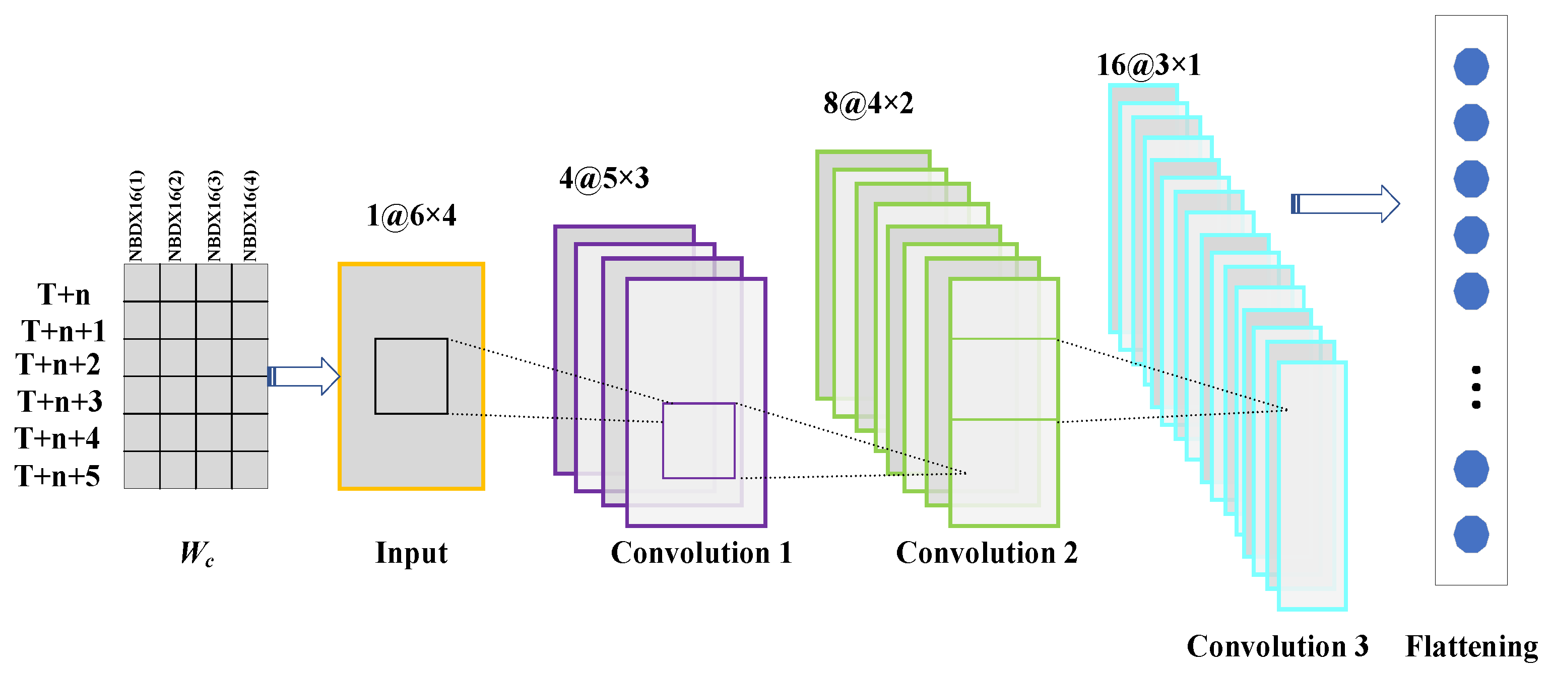
3.3.1. Implementation of the CNN Model

CNN models have been applied in many fields, which can effectively capture local feature information between data. CNN models consist of an input layer, convolutional layer, pooling layer and output layer. Local perception and weight sharing can be achieved through convolutional processing [41]. CNNs are mainly employed to obtain the spatial features of traffic flow data.

Three convolutional layers and one flat layer constitute the CNN model used in this article. The input values were fed into the filter to perform a convolution operation. The channels of convolutional layers were set to 4, 8, and 16, respectively. The convolutional process is exhibited in Figure 2. The CNN model in this paper was configured by referring to [20]. The computation of the convolution process is shown in Formula (18):

$$Y_j^k=f\left({\displaystyle \sum _{i\in N_j}{x}_i^{k-1}{u}_{ij}+b_j^k}\right)$$

(18)

where $Y_j^k$ and $x_i^{k-1}$ denote the inputs and outputs, $f\left(\cdot \right)$ denotes the activation function, $i$ and $j$ denote the processing positions in the convolution process, $u_{ij}$ denotes the weight of the convolutional kernel, $b_j^k$ is the bias parameter and $N_j$ denotes the input features.

In addition, to solve the gradient explosion and vanishing due to the increase in the depth of the network structure, residual units were introduced, as shown in Formula (19).

$$X_c^k=X_c^{\left(k-1\right)}+\vartheta \left(X_c^k;{\theta }_c^k\right)$$

(19)

where $k=1,2,\cdots ,M$, $\vartheta$ is the residual function, and ${\theta }_c^k$ is all the parameters that can be learnt by the kth layer residual unit.

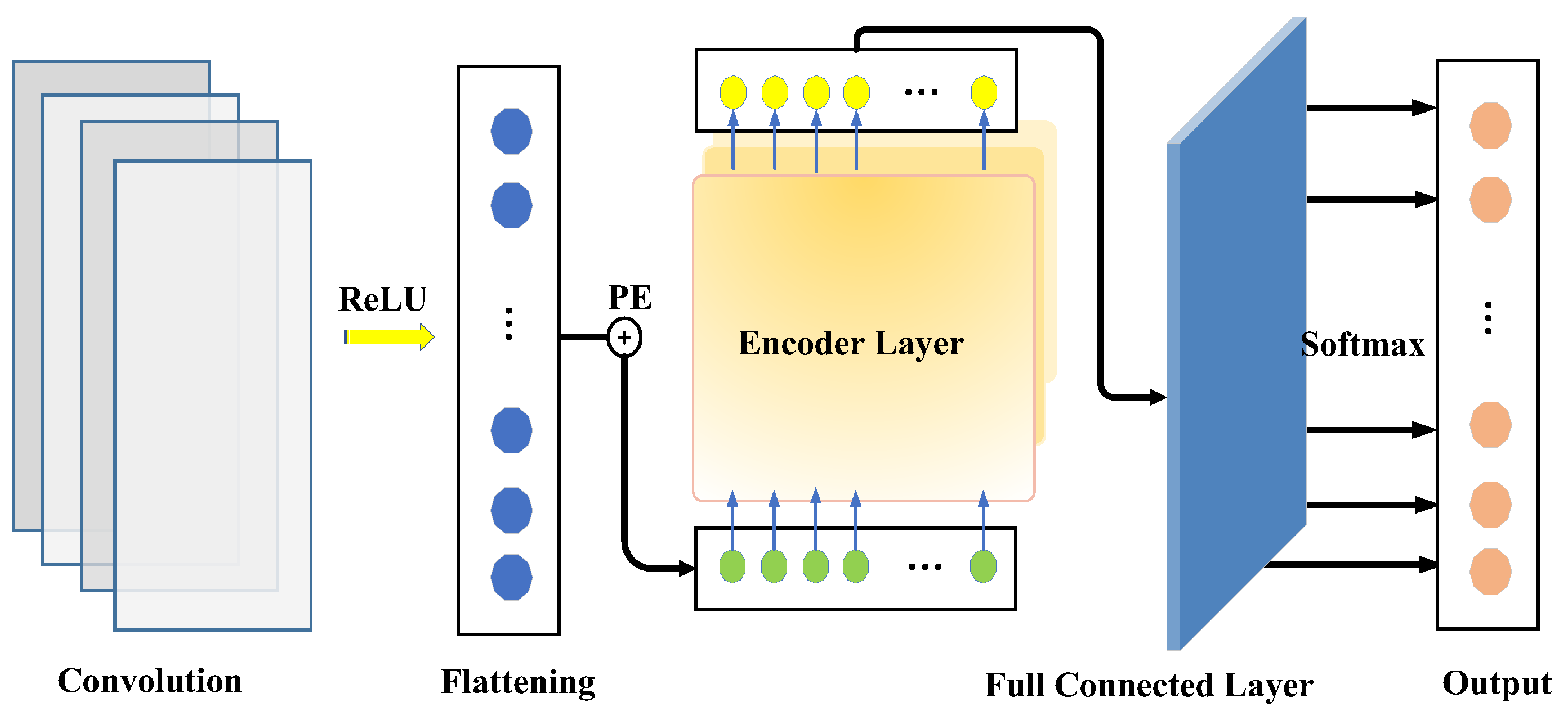
3.3.2. Implementation of the Transformer

Numerous experiments have been conducted to demonstrate that this is an excellent deep learning model [42]. This paper utilizes the Transformer model to further extract features from the time dimension and to handle traffic flow forecasting. Compared with RNN-based models, the Transformer model can more effectively identify the intrinsic relationships of time series data. The Transformer model abandons the typical neural network architecture and employs an attention mechanism for machine translation tasks, which enhances the focus and utilization of important information, allowing for the direct acquisition of global information without the need for step-by-step recursion. It also enables parallel computing, significantly reducing computational time, and improving both training efficiency and prediction accuracy.

The Transformer model includes an encoder and a decoder, which mainly comprise three components: input, multi-head attention and fully connected feed-forward networks. The structure is described in Figure 3.

The encoder and decoder have certain differences in functionality; the encoder typically has only one input, while the decoder has two inputs. When making time series predictions, only the encoder is utilized for time series forecasting, and the fully connected layer can replace the functionality of the decoder. Since the attention mechanism of the Transformer can acquire all input data simultaneously, disregarding the sequential information between data points, it requires positional encoding to provide the relative positional information of input data. Formulas (20) and (21) give the encoding principles.

$$P{E}_{\left(pos,2i\right)}=\sin \left(pos/{10000}^{2i/d_{\mathrm{mod}\mathrm{el}}}\right)$$

(20)

$$P{E}_{\left(pos,2i\right)}=\cos \left(pos/{10000}^{2i/d_{\mathrm{model}}}\right)$$

(21)

where pos indicates the position index and $d_{\mathrm{model}}$ is data dimensionality.

After positional encoding, the input data are fed into the encoder component of the Transformer. The encoder consists of a multi-head attention mechanism, residual connection, layer normalization and a feed-forward network. Firstly, the input vectors are subjected to cubic linear transformations, and query vector Q, key vector K and value vector V are generated. Subsequently, the matrix V is weighted and summed by using the correlation between Q and K to obtain the output value of self-attention. Eventually, different attention results are concatenated. The procedure is represented by Formulas (22) and (23). Figure 4 gives the schematic diagram of the multi-head attention mechanism.

$$\begin{array}{c}\mathrm{MultiHead}\left(Q,K,V\right)=\mathrm{Conact}\left({\mathrm{head}}_1{,\mathrm{head}}_2,\cdots {,\mathrm{head}}_{\mathrm{n}}\right)W^O\\ {\mathrm{where}\mathrm{head}}_{\mathrm{i}}=\mathrm{Attention}\left(Q{W}_i^Q,K{W}_i^K,V{W}_i^V\right)\end{array}$$

(22)

where $W_i^Q,W_i^K$ and $W_i^V$ are the linear transformation weight matrices, $W_i^Q\in {ℝ}^{d_m\times d_q},W_i^K\in {ℝ}^{d_m\times d_k},W_i^V\in {ℝ}^{d_m\times d_v},W^O\in {ℝ}^{{ }_{h{d}_v\times d_m}}$, $d_{\mathrm{model}}=h{d}_{k,}{d}_k=d_v$. Attention is obtained from Formula (24).

$$\mathrm{Attention}(Q,K,V)=\mathrm{SoftMax}\left(\frac{Q{K}^T}{\sqrt{d_k}}\right)V$$

(23)

The output of the attention mechanism is fed into the feed-forward network, and the residual concatenation and normalization operations are performed to acquire results. Finally, the output values of the encoder layers are transmitted to decoder layers composed of fully connected layers. These processed data are then fitted to acquire the final results.

3.4. The Architecture of the CEEMDAN-VMD-CNN–Transformer Model

We developed a short-term traffic flow forecasting approach combining a secondary decomposition strategy and a CNN–Transformer model. Figure 5 gives the architecture of the presented method. The proposed approach consists of the following steps:

Step 1: Traffic flow data are decomposed by applying the CEEMDAN algorithm, and several high-frequency subsequences and a low-frequency subsequence are obtained.

Step 2: The highest-frequency subsequences are further decomposed into some stationary IMFs using the VMD algorithm. The VMD lever is determined by the values of the center frequency.

Step 3: The CNN–Transformer models are trained with each IMF component acquired from the CEEMDAN-VMD, and different CNN–Transformer models are built to forecast each IMF component.

Step 4: Three-step-ahead forecasting is executed for each forecasting model. Three-step-ahead predictions are performed by using the logic of iterative multi-step forecasting. Step 5: The final prediction results are obtained by superimposing each sub-component’s forecasting result.

4. Experimental Verification

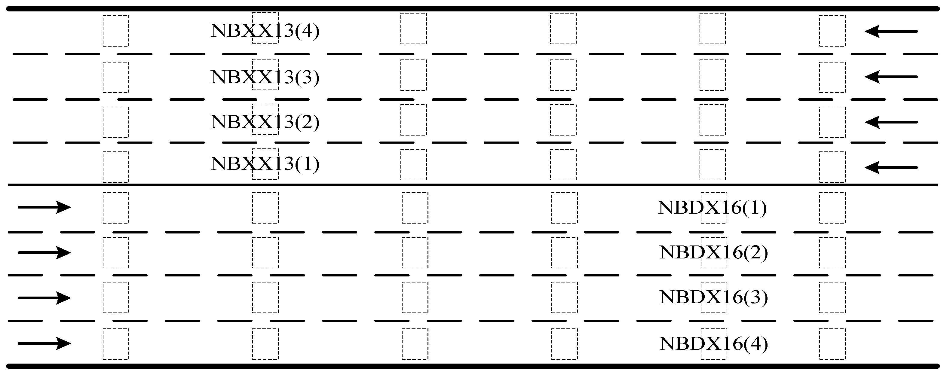
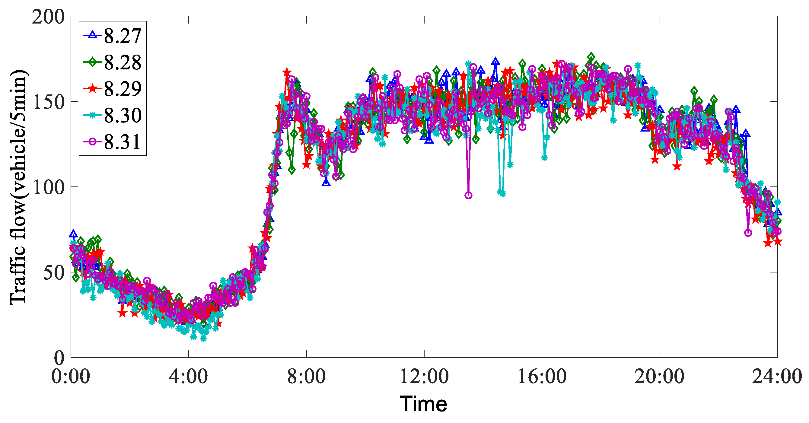
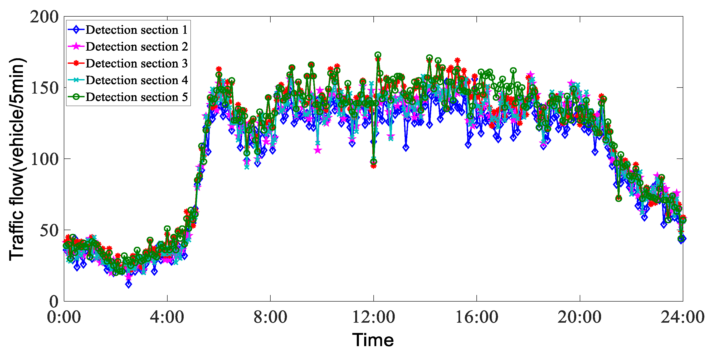
4.1. Data Source

A section of urban expressway in Shanghai was selected as the experimental section. There are four lanes in each direction on this expressway, and the schematic diagram of detector deployment is shown in Figure 6. The selected road section included 24 detection sections on the main line. There were a total of 88 mainline detectors. The distance between adjacent detection cross-sections was 500 m. The data were collected on 27 August, 28 August, 29 August, 30 August and 31 August in 2018. The data collection time interval was 5 min.

Figure 7 displays the measured traffic flow data of the expressway for five consecutive days, which reflects the long-term trend of traffic flow data. There is generally a relatively stable pattern of socio-economic activities in specific regions. For example, activities such as going to work and school have a certain regularity in time distribution, resulting in strong temporal correlations in the traffic flow data. Figure 8 displays the measured traffic flow data for adjacent detection cross-sections. Figure 9 displays the measured traffic flow data for adjacent lanes. The expressway traffic flow is continuous, and exhibits a strong spatial correlation. From Figure 7, Figure 8 and Figure 9, we can see that the short-term traffic flow data display strong similarity, which is a prerequisite for building a traffic flow forecasting model.

4.2. Evaluating Indicators

The following indicators were employed as evaluation indicators for the effectiveness of traffic flow forecasting:

$$RMSE=\sqrt{\frac{1}{n}{\displaystyle {\sum }_{i=1}^n{\left(y_i-{\widehat{y}}_i\right)}^2}}$$

(24)

$$MAE=\frac{1}{n}{\displaystyle {\sum }_{i=1}^n\left|y_i-{\widehat{y}}_i\right|}$$

(25)

$$MAPE=\frac{1}{n}{\displaystyle {\sum }_{i=1}^n\left|\frac{y_i-{\widehat{y}}_i}{y_i}\right|}\times 100\%$$

(26)

where $y_i$ is the measured data, ${\widehat{y}}_i$ is the forecasting result and n is the sample size.

To quantitatively describe the degree of enhancement of the proposed approach, enhancement percentages such as P_RMSE, P_MAE and P_MAPE were employed.

$$P_{RMSE}=\left(\frac{RMS{E}_1-RMS{E}_2}{RMS{E}_1}\right)\times 100\%$$

(27)

$$P_{MAE}=\left(\frac{MA{E}_1-MA{E}_2}{MA{E}_1}\right)\times 100\%$$

(28)

$$P_{MAPE}=\left(\frac{MAP{E}_1-MAP{E}_2}{MAP{E}_1}\right)\times 100\%$$

(29)

where a subscripted 1 indicates the comparative method and subscripted 2 indicates the proposed method.

4.3. CEEMDAN Results

During the CEEMDAN process, the standard deviation of Gaussian white noise was set to 0.1, the number of times that noise was added was 100, and the maximum number of sifting iterations was 10. The CEEMDAN results of the NBDX16(2) and NBXX11(3) datasets are shown in Figure 10 and Figure 11, respectively. NBDX16(2) and NBXX11(3) are the number index of the detectors, 16 and 11 represent the numbers of the detector’s cross-sections, and (2) and (3) indicate the number of lanes in each detector’s cross-section.

It can be seen that the IMF1 obtained from CEEMDAN expresses stronger volatility and randomness than other IMFs, which increases the forecasting difficulty to some extent. To solve the IMF1 issues, the IMF1 was further decomposed into several sub-series by applying the VMD algorithm.

4.4. VMD Results

In the process of secondary decomposition, the IMF1 sub-layer is further decomposed into several sub-series by VMD. The values of the central frequency of each sub-component were calculated to determine the decomposition level. The appropriate decomposition level was used until the change of central frequency is not significant. Values were set to $\alpha =2200$, $\tau =0.25$, $\epsilon ={10}^{-6}$.

Table 2. The values of center frequency for the NBDX16(2) dataset.

K	IMF1	IMF2	IMF3	IMF4	IMF5
2	185.17	292.64
3	180.14	268.48	341.76
4	193.05	260.56	321.41	343.09
5	186.98	244.83	289.09	327.86	347.96

and

Table 3. The values of center frequency for the NBXX11(3) dataset.

K	IMF1	IMF2	IMF3	IMF4	IMF5
2	179.06	299.62
3	198.08	289.18	381.06
4	193.03	264.87	326.54	383.22
5	181.20	242.28	302.06	332.37	386.50

show the values of the center frequency for each IMF under different numbers of decomposition layers.

From Table 2 and Table 3, we can see that the change in central frequency values is not significant when the decomposition level exceeds 3. Hence, the VMD level was selected as 3.

Figure 12 and Figure 13 show the decomposition results and the corresponding frequency spectrum of VMD.

In Figure 12 and Figure 13, the display on the left shows the secondary decomposition results, and the right side shows the corresponding frequency spectrum.

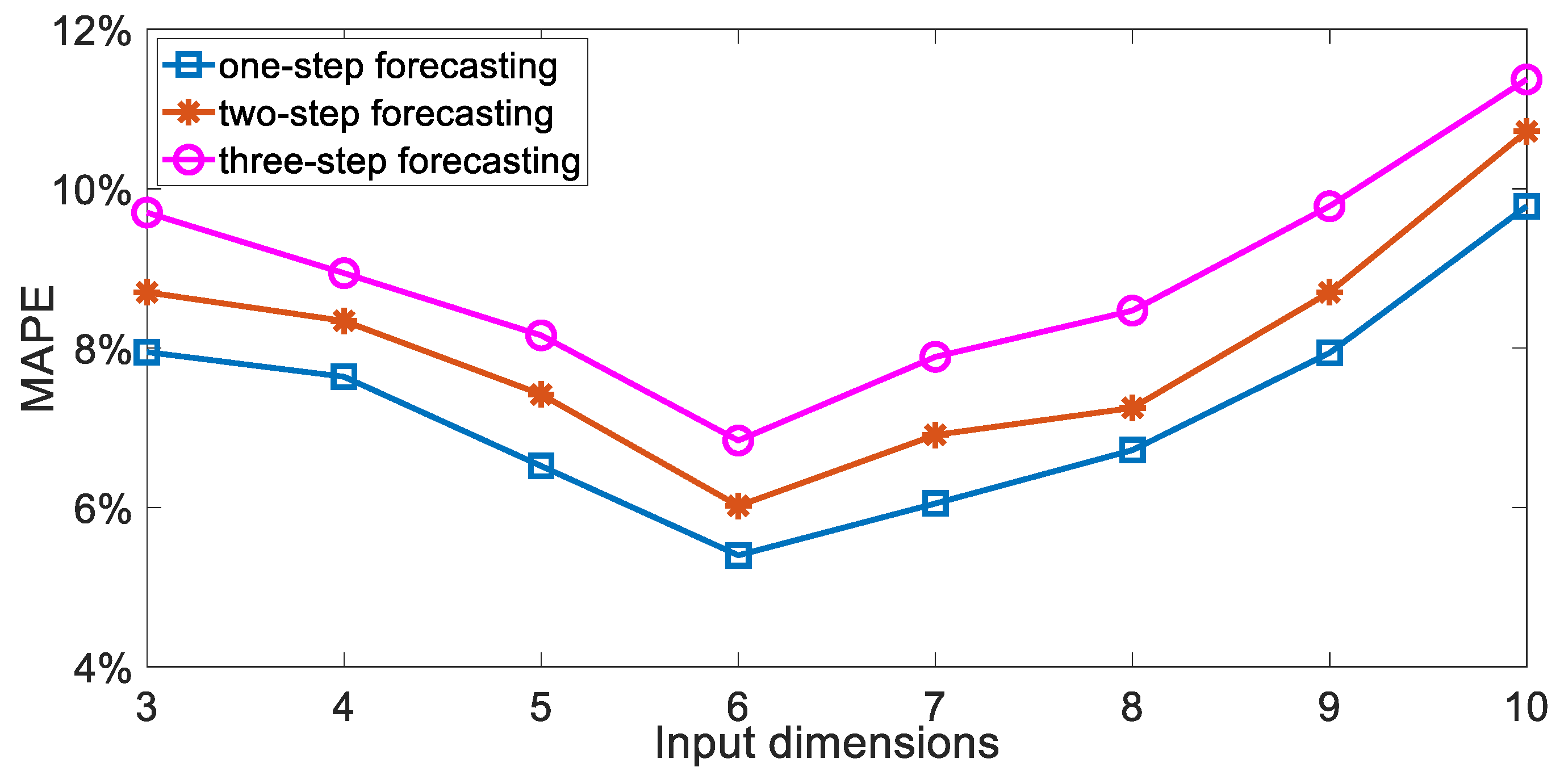
4.5. Selection of Input Dimension

The input dimension is one of the critical parameters. The MAPE values of different input dimensions are shown in Figure 14. The forecasting error reaches the minimum when the input dimension is set to 6. Hence, we set the input dimension to 6 for the experiment.

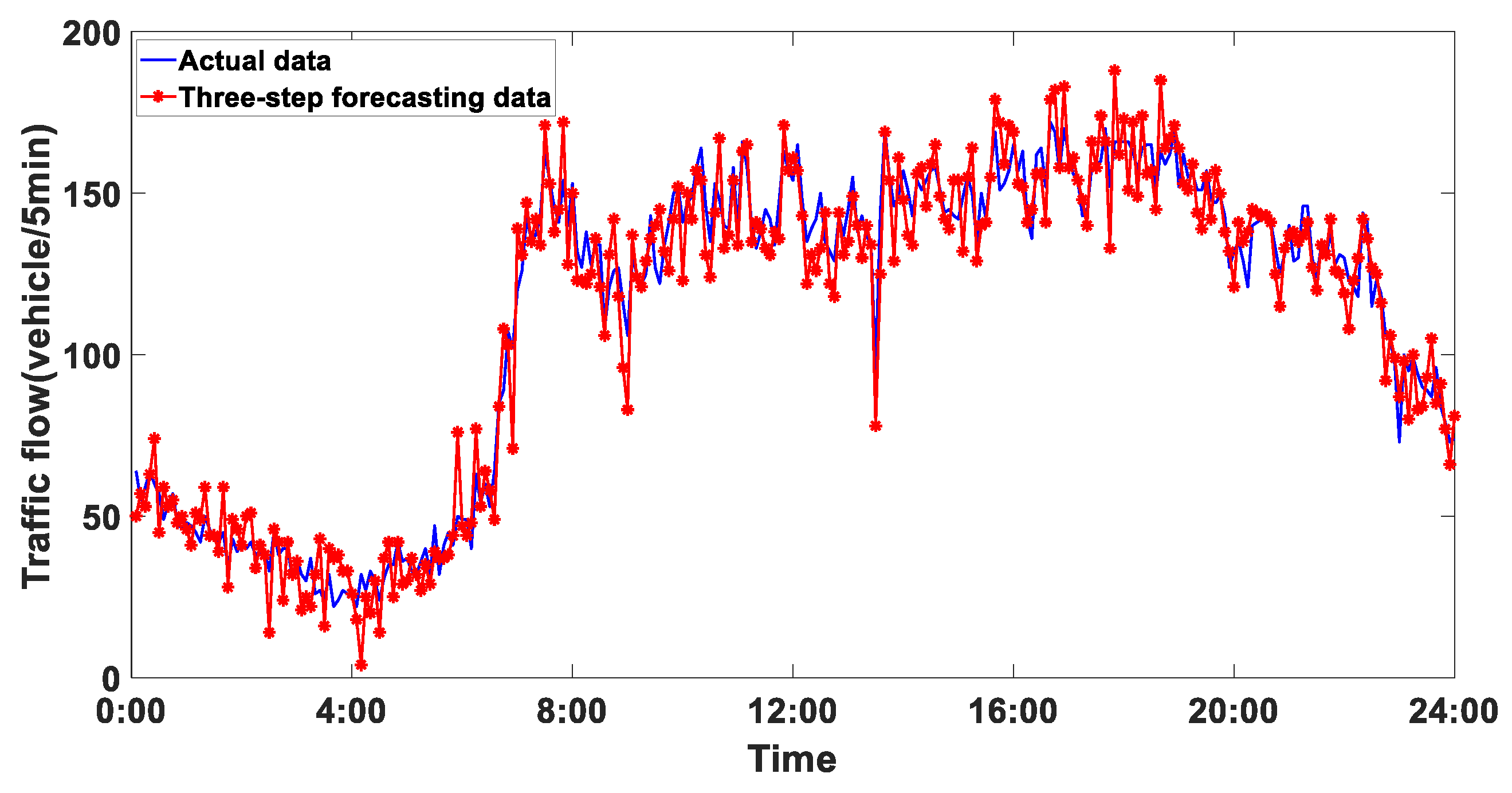
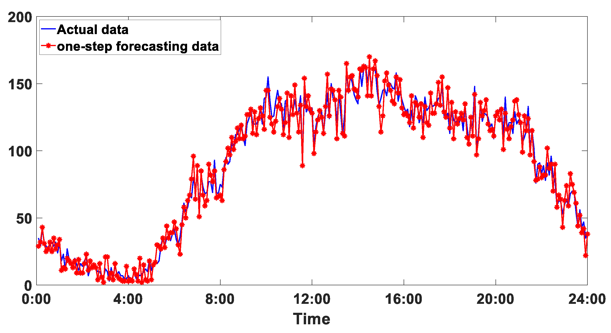
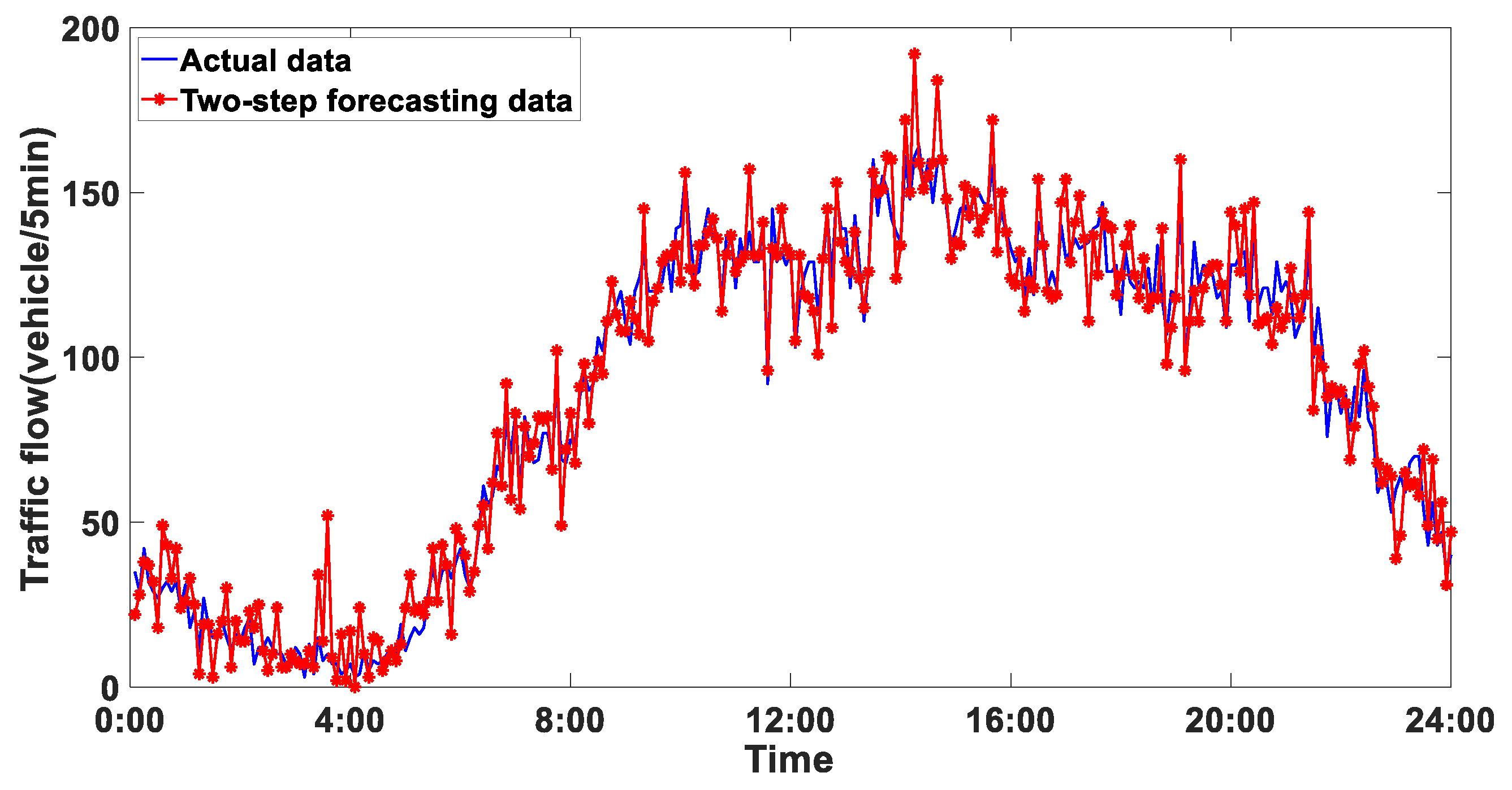
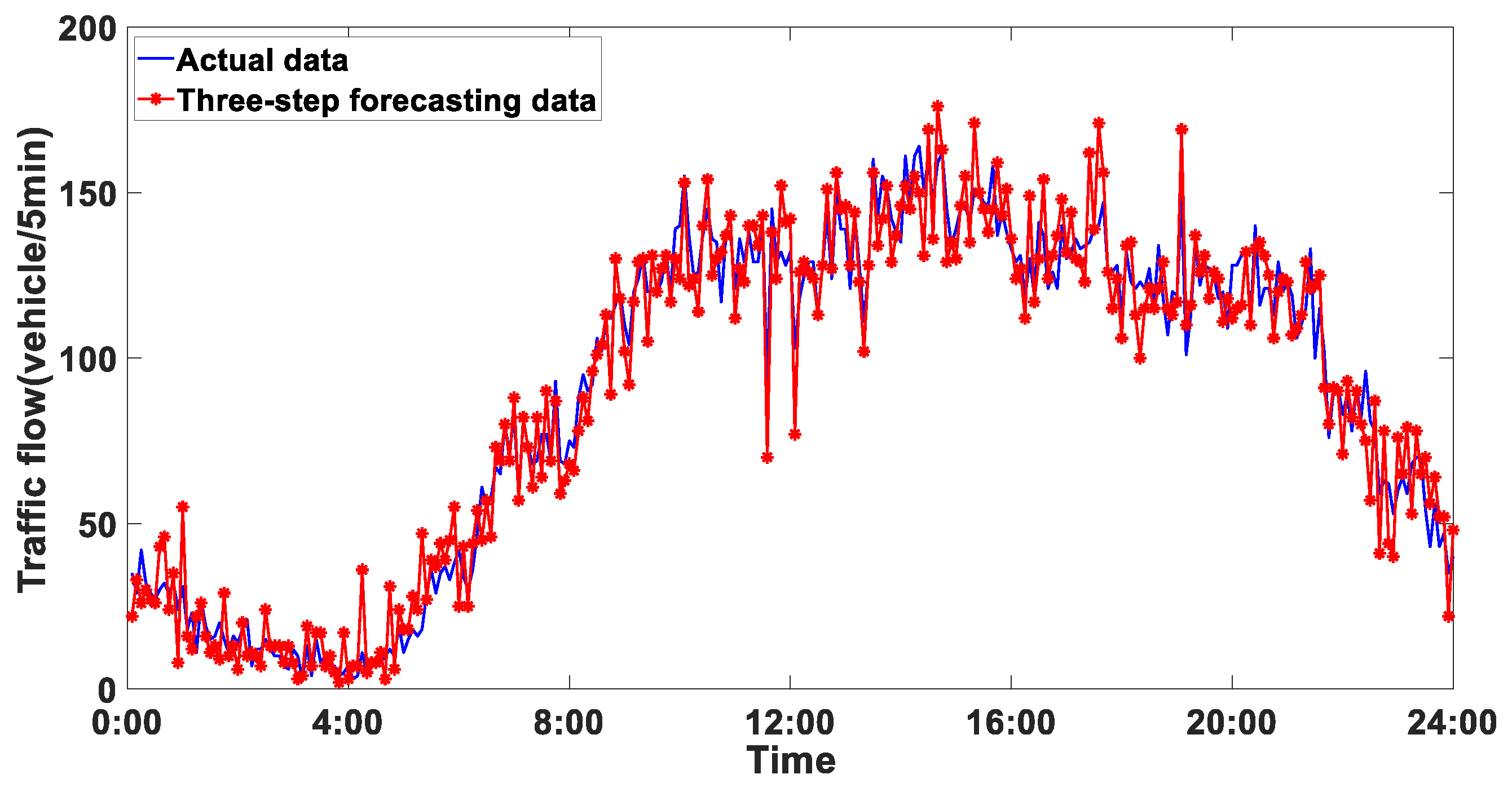
4.6. Analysis of Experimental Results

Three-step-ahead predictions were carried out to check the predictive performance. According to different multi-step prediction logics, multi-step forecasting includes iterative forecasting and direct forecasting. Iterative forecasting was employed in this study. The logic of iterative multi-step forecasting is shown in Figure 15; when forecasting ${\widehat{y}}_{t+2}$, the input data are $\left\{y_{t-p+1},\cdots ,y_t,{\widehat{y}}_{t+1}\right\}$.

After repeated training of the model and continuous adjustments to its parameters, optimal performance was achieved for the CNN–Transformer model. The specific parameters of CNN–Transformer are displayed in

Table 4. Parameter settings for CNN–Transformer.

Parameters	Value
Epochs	300
Batch size	64
Learning rate	0.0012
Convolutional kernel size	2 × 2
Encoder layer	3
Decoder (fully connected layer)	3
Attention head	6
Dropout rate	0.2
Optimizer	Adam
Loss function	RMSE

. Figure 16, Figure 17, Figure 18, Figure 19, Figure 20 and Figure 21 give the three-step-ahead forecasting results of the NBDX16(2) and NBXX11(3) datasets, respectively.

In Figure 16, Figure 17, Figure 18, Figure 19, Figure 20 and Figure 21, the blue line expresses measured data and the red line with an asterisk expresses the forecasting values. The forecasting results captured the fluctuation trends of traffic data well, while the error between the forecasting results and measured values was relatively small. Therefore, the prediction results show that the CEEMDAN-VMD-CNN–Transformer method could achieve excellent forecasting accuracy.

5. Comparison and Discussion

To evaluate generalization ability and reliability, five-fold cross-validation experimental tests were conducted. The experimental data were separated into five parts. For each experiment, four parts were applied to train the proposed CNN–Transformer, and the remaining part served as the testing dataset. The average of five experimental results was treated as the final result. Figure 22 gives the schematic diagram of the five-fold cross-validation.

Five other methods, including CNN–Transformer, CEEMDAN-CNN–Transformer, VMD-CNN–Transformer, CEEMDAN-VMD-CNN and CEEMDAN-VMD–Transformer were considered in a comparison to demonstrate the superiority of the proposed method. All involved methods were tested on three-step-ahead prediction experiments. MatlabR2023a was utilized in this paper to test the proposed models.

Table 5. Comparison of forecasting errors for NBDX16(2) dataset.

Methods	Evaluation Indicators	1-Step	2-Step	3-Step
CNN–Transformer	MAE	9.42	10.17	12.38
	RMSE	42.74	44.53	47.25
	MAPE	11.12%	13.07%	14.62%
CEEMDAN-CNN–Transformer	MAE	8.01	8.52	9.14
	RMSE	39.08	42.75	44.27
	MAPE	9.01%	9.63%	10.15%
VMD-CNN–Transformer	MAE	7.04	8.01	8.77
	RMSE	38.24	41.10	42.54
	MAPE	7.12%	7.82%	8.67%
CEEMDAN-VMD-CNN	MAE	5.04	5.57	6.22
	RMSE	36.08	38.84	41.20
	MAPE	6.11%	6.82%	7.57%
CEEMDAN-VMD-Transformer	MAE	4.51	5.02	5.93
	RMSE	34.66	37.12	39.34
	MAPE	5.37%	6.28%	7.11%
CEEMDAN-VMD-CNN–Transformer	MAE	4.06	4.75	5.38
	RMSE	32.07	34.20	37.12
	MAPE	5.28%	6.01%	6.73%

and

Table 6. Comparison of forecasting errors for NBXX11(3) dataset.

Methods	Evaluation Indicators	1-Step	2-Step	3-Step
CNN–Transformer	MAE	9.74	10.85	13.26
	RMSE	43.55	46.14	49.02
	MAPE	12.20%	13.96%	15.79%
CEEMDAN-CNN–Transformer	MAE	8.14	9.02	9.46
	RMSE	39.31	42.75	44.84
	MAPE	9.07%	9.58%	10.21%
VMD-CNN–Transformer	MAE	7.17	8.48	9.16
	RMSE	38.15	41.23	43.08
	MAPE	7.14%	8.26%	8.77%
CEEMDAN-VMD-CNN	MAE	5.10	5.72	6.27
	RMSE	36.12	39.43	41.87
	MAPE	6.17%	7.25%	8.06%
CEEMDAN-VMD-Transformer	MAE	4.58	5.47	6.02
	RMSE	34.83	37.15	40.14
	MAPE	5.78%	7.01%	7.58%
CEEMDAN-VMD-CNN–Transformer	MAE	4.25	5.06	5.74
	RMSE	33.20	35.12	38.30
	MAPE	5.33%	6.14%	6.85%

give the comparison of the forecasting errors for the NBDX16(2) and NBXX11(3) datasets.

From the forecasting errors of the different methods shown in Table 5 and Table 6, we reached the following conclusions:

(1)

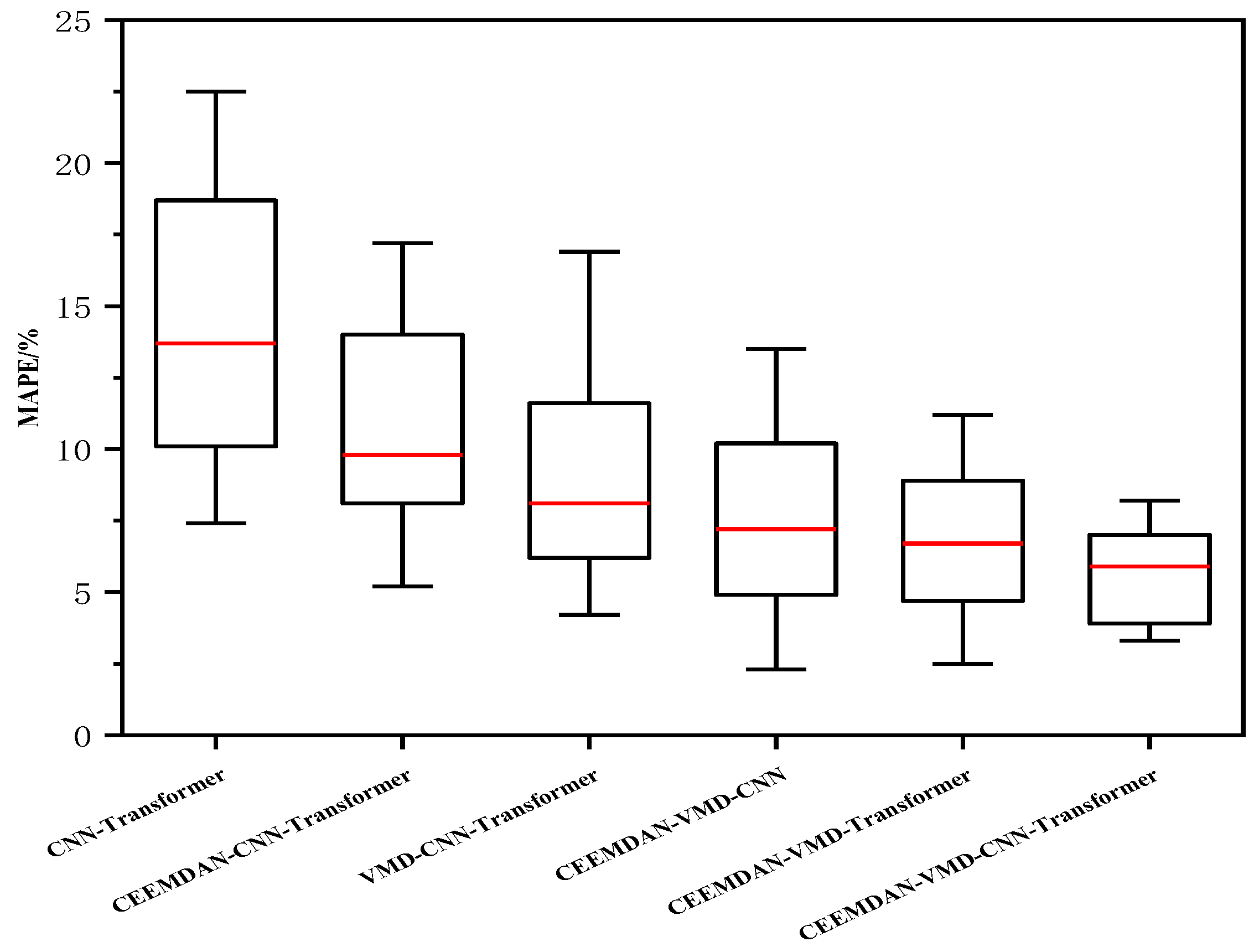
The methods considering data decomposition have better forecasting performance than forecasting methods without data decomposition algorithms. Taking the comparison of the CNN–Transformer method and CEEMDAN-VMD-CNN–Transformer method as an example, the CEEMDAN-VMD-CNN–Transformer method declined by 56.90%, 53.29% and 56.54% in three-step-ahead forecasting for the NBDX16(2) dataset in terms of MAE; by 24.96%, 23.20% and 21.44% in three-step-ahead forecasting in terms of RMSE; and by 52.52%, 54.02% and 53.97% in three-step-ahead forecasting in terms of MAPE.

(2)

The forecasting performance of the CEEMDAN-VMD-CNN–Transformer method obviously outperformed the CEEMDAN-CNN–Transformer and VMD-CNN–Transformer methods, which shows that the proposed secondary decomposition strategy is significantly effective. Taking the comparison of the CEEMDAN-CNN–Transformer method and CEEMDAN-VMD-CNN–Transformer method as an example, the CEEMDAN-VMD-CNN–Transformer method declined by 49.31%, 44.25% and 36.76% in three-step-ahead forecasting for the NBDX16(2) dataset in terms of MAE; by 17.94%, 20% and 16.15% in three-step-ahead forecasting for the NBDX16(2) dataset in terms of RMSE; and by 41.40%, 37.59% and 33.69% in three-step-ahead forecasting for the NBDX16(2) dataset in terms of MAPE. Taking the comparison of the VMD-CNN–Transformer and CEEMDAN-VMD-CNN–Transformer methods as an example, the CEEMDAN-VMD-CNN–Transformer method declined by 42.33%, 40.70% and 34.09% in three-step-ahead forecasting for the NBDX16(2) dataset in terms of MAE; by 16.13%, 16.79% and 12.74% in three-step-ahead forecasting for the NBDX16(2) dataset in terms of RMSE; and by 25.84%, 23.15% and 22.38% in three-step -head forecasting for the NBDX16(2) dataset in terms of MAPE.

(3)

The forecasting results of the CEEMDAN-VMD-CNN–Transformer method outperforms the CEEMDAN-VMD-Transformer and CEEMDAN-VMD-CNN models, which proves that the cascaded CNN–Transformer model can match the features of traffic flow data wonderfully. Taking the comparison of the CEEMDAN-VMD-CNN method and the CEEMDAN-VMD-CNN–Transformer method as an example, the CEEMDAN-VMD-CNN–Transformer method declined by 19.44%, 14.72% and 13.50% in three-step-ahead forecasting for the NBDX16(2) dataset in terms of MAE; by 11.11%, 11.95% and 9.90% in three-step-ahead forecasting for the NBDX16(2) dataset in terms of RMSE; and by 13.58%, 11.88% and 11.10% in three-step-ahead forecasting for the NBDX16(2) dataset in terms of MAPE. Taking the comparison of the CEEMDAN-VMD-Transformer method and the CEEMDAN-VMD-CNN–Transformer method as an example, the CEEMDAN-VMD-CNN–Transformer method declined by 9.98%, 5.38% and 9.27% in three-step-ahead forecasting for the NBDX16(2) dataset in terms of MAE; by 5.65%, 7.87% and 5.64% in three-step-ahead forecasting for the NBDX16(2) dataset in terms of RMSE; and by 1.68%, 4.30% and 5.34% in three-step-ahead forecasting for the NBDX16(2) dataset in terms of MAPE.

(4)

The proposed CEEMDAN-VMD-CNN–Transformer method has significant advantages over other comparative methods for three-step-ahead forecasting.

Figure 23, Figure 24 and Figure 25 are the boxplots of MAPE for the different forecasting methods. The top of the box indicates the 75th Quantile, the bottom of the box indicates the 25th Quantile and the red line in the box indicates the median. The distance between the 75th Quantile and 25th Quantile is called the Inter-Quartile Range (IQR), which is used to measure the concentration of errors. Extension lines refer to the maximum and minimum except for outliers. The IQR for the proposed CEEMDAN-VMD-CNN–Transformer method is minimal in terms of MAPE, which shows that the CEEMDAN-VMD-CNN–Transformer method shows outstanding stability.

6. Conclusions

This paper developed a novel short-term traffic flow forecasting approach by applying a secondary decomposition strategy and a CNN–Transformer model. Traffic flow data were firstly decomposed by using the CEEMDAN algorithm, and a series of IMFs were obtained. Then, the IMF1 obtained from CEEMDAN was further decomposed into some sub-series by using the VMD algorithm. It has been proven that the secondary decomposition strategy can effectively solve the high volatility and randomness problems of IMF1. The CNN–Transformer was established for each IMF separately, and the final results were obtained by superimposing each sub-component’s forecasting results. Finally, three-step-ahead forecasting was conducted, and the traffic flow data of urban expressways were applied for experimental verification. The experimental results show that the CEEMDAN-VMD-CNN–Transformer method could achieve excellent forecasting accuracy and has significant advantages over other comparative methods.

For future research, the complexity of each intrinsic mode function obtained from the first decomposition algorithm could be quantified, and high-complexity components can be merged and then subjected to secondary decomposition. In addition, some improved attention mechanisms could be added to improve the forecasting performance of CNN–Transformer. Meanwhile, parallel structures can be adopted to accelerate model training and inference speed.

References

1. Ji, J.H.; Bie, Y.M.; Wang, L.H. Optimal electric bus fleet scheduling for a route with charging facility sharing. Transp. Res. Part C Emerg. Technol. 2023, 147, 104010. [Google Scholar] [CrossRef]
2. Zhang, Y.R.; Zhang, Y.L.; Ali, H. A hybrid short-term traffic flow forecasting method based on spectral analysis and statistical volatility model. Transp. Res. Part C 2014, 43, 65–78. [Google Scholar] [CrossRef]
3. Lin, X.; Huang, Y. Short-term high-speed traffic flow prediction based on ARIMA-GARCH-M model. Wirel. Pers. Commun. 2021, 117, 3421–3430. [Google Scholar] [CrossRef]
4. Li, D. Predicting short-term traffic flow in urban based on multivariate linear regression model. J. Intell. Fuzzy Syst. 2020, 39, 1417–1427. [Google Scholar] [CrossRef]
5. Zhou, T.; Jiang, D.; Lin, Z.; Han, G.; Xu, X.; Qin, J. Hybrid dual Kalman filtering model for short-term traffic flow forecasting. IET Intell. Transp. Syst. 2019, 13, 1023–1032. [Google Scholar] [CrossRef]
6. Xu, X.; Jin, X.; Xiao, D.; Ma, C.; Wong, S.C. A hybrid autoregressive fractionally integrated moving average and nonlinear autoregressive neural network model for short-term traffic flow prediction. J. Intell. Transp. Syst. 2023, 27, 1–18. [Google Scholar] [CrossRef]
7. Peng, Y.N.; Xiang, W.L. Short-term traffic volume forecasting using GA-BP based on wavelet denoising and phase space reconstruction. Physica A 2020, 549, 123913. [Google Scholar] [CrossRef]
8. Ma, C.X.; Tan, L.M.; Xu, X.C. Short-term traffic flow prediction based on genetic artificial neural network and exponential smoothing. Promet-Traffic Transp. 2020, 32, 747–760. [Google Scholar] [CrossRef]
9. Xu, L.Q.; Du, X.D.; Wang, B.G. Short-term traffic flow prediction model of wavelet neural network based on mine evolutionary algorithm. Int. J. Pattern Recognit. Artif. Intell. 2018, 32, 1850041. [Google Scholar] [CrossRef]
10. Feng, X.; Ling, X.; Zheng, H.; Chen, Z.; Xu, Y. Adaptive multi-kernel SVM with spatial-temporal correlation for short-term traffic flow prediction. IEEE Trans. Intell. Transp. Syst. 2019, 20, 2001–2013. [Google Scholar] [CrossRef]
11. Toan, T.D.; Truong, V.H. Support vector machine for short-term traffic flow prediction and improvement of its model training using nearest neighbor approach. Transp. Res. Rec. 2021, 2675, 362–373. [Google Scholar] [CrossRef]
12. Yang, Y.; Li, Z.; Chen, J.; Liu, Z.; Cao, J. TRELM-DROP: An impavement non-iterative algorithm for traffic flow forecast. Phys. A Stat. Mech. Its Appl. 2024, 633, 129337. [Google Scholar] [CrossRef]
13. Bing, Q.; Shen, F.; Chen, X.; Zhang, W.; Hu, Y.; Qu, D. A hybrid short-term traffic flow multistep prediction method based on variational mode decomposition and long short-term memory model. Discret. Dyn. Nat. Soc. 2021, 2021, 4097149. [Google Scholar] [CrossRef]
14. Huang, H.-C.; Chen, J.-Y.; Shi, B.-C.; He, H.-D. Multi-step forecasting of short-term traffic flow based on Intrinsic Pattern Transform. Phys. A Stat. Mech. Its Appl. 2023, 621, 128798. [Google Scholar] [CrossRef]
15. Chen, X.; Lu, J.; Zhao, J.; Qu, Z.; Yang, Y.; Xian, J. Traffic flow prediction at varied time scales via ensemble empirical mode decomposition and artificial neural network. Sustainability 2020, 12, 3678. [Google Scholar] [CrossRef]
16. Zheng, Y.; Wang, S.; Dong, C.; Li, W.; Zheng, W.; Yu, J. Urban road traffic flow prediction: A graph convolutional network embedded with wavelet decomposition and attention mechanism. Phys. A Stat. Mech. Its Appl. 2022, 608, 128274. [Google Scholar] [CrossRef]
17. Wu, X.Y.; Fu, S.D.; He, Z.J. Research on short-term traffic flow combination prediction based on CEEMDAN and machine learning. Appl. Sci. 2023, 13, 308. [Google Scholar] [CrossRef]
18. Yang, H.; Cheng, Y.X.; Li, G.H. A new traffic flow prediction model based on cosine similarity variational mode decomposition, extreme learning machine and iterative error compensation strategy. Eng. Appl. Artif. Intell. 2022, 115, 105234. [Google Scholar] [CrossRef]
19. Liu, H.; Tian, H.-Q.; Liang, X.-F.; Li, Y.-F. Wind speed forecasting approach using secondary decomposition algorithm and Elman neural networks. Appl. Energy 2015, 157, 183–194. [Google Scholar] [CrossRef]
20. Yin, H.; Ou, Z.; Huang, S.; Meng, A. A cascaded deep learning wind power prediction approach based on a two-layer of mode decomposition. Energy 2019, 189, 116316. [Google Scholar] [CrossRef]
21. Sun, W.; Tan, B.; Wang, Q.Q. Multi-step wind speed forecasting based on secondary decomposition algorithm and optimized back propagation neural network. Appl. Soft Comput. 2021, 113, 107894. [Google Scholar] [CrossRef]
22. Wen, Y.; Pan, S.; Li, X.; Li, Z. Highly fluctuating short-term load forecasting based on improved secondary decomposition and optimized VMD. Sustain. Energy Grids Netw. 2024, 37, 101270. [Google Scholar] [CrossRef]
23. Zhang, G.; Zhang, Y.; Wang, H.; Liu, D.; Cheng, R.; Yang, D. Short-term wind speed forecasting based on adaptive secondary decomposition and robust temporal convolutional network. Energy 2024, 288, 129618. [Google Scholar] [CrossRef]
24. Zhao, L.; Wen, X.; Shao, Y.; Tang, Z. Hybrid model for method for short-term traffic flow prediction based on secondary decomposition technique and ELM. Math. Probl. Eng. 2022, 2022, 9102142. [Google Scholar] [CrossRef]
25. Hu, G.; Whalin, R.W.; Kwembe, T.A.; Lu, W. Short-term traffic flow prediction based on secondary hybrid decomposition and deep echo state networks. Phys. A Stat. Mech. Its Appl. 2023, 632, 129313. [Google Scholar] [CrossRef]
26. Li, H.; Jin, F.; Sun, S.; Li, Y. A new secondary decomposition ensemble learning approach for carbon price forecasting. Knowl.-Based Syst. 2021, 214, 106686. [Google Scholar] [CrossRef]
27. Li, J.M.; Liu, D.H. Carbon price forecasting based on secondary decomposition and feature screening. Energy 2023, 278, 127783. [Google Scholar] [CrossRef]
28. Do, L.N.; Vu, H.L.; Vo, B.Q.; Liu, Z.; Phung, D. An effective spatial-temporal attention based neural network for traffic flow prediction. Transp. Res. Part C Emerg. Technol. 2019, 108, 12–28. [Google Scholar] [CrossRef]
29. Zhang, W.; Yu, Y.; Qi, Y.; Shu, F.; Wang, Y. Short-term traffic flow prediction based on spatio-temporal analysis and CNN deep learning. Transp. A Transp. Sci. 2019, 15, 1688–1711. [Google Scholar] [CrossRef]
30. Ma, D.F.; Song, X.; Li, P. Daily Traffic Flow Forecasting through a Contextual Convolutional Recurrent Neural Network Modeling Inter- and Intra-Day Traffic Patterns. IEEE Trans. Intell. Transp. Syst. 2020, 22, 2627–2636. [Google Scholar] [CrossRef]
31. Chen, Y.; Chen, X.Q. A novel reinforced dynamic graph convolutional network model with data imputation for network-wide traffic flow prediction. Transp. Res. Part C Emerg. Technol. 2022, 143, 103820. [Google Scholar] [CrossRef]
32. Redhu, P.; Kumar, K. Short-term traffic flow prediction based on optimized deep learning neural network: PSO-Bi-LSTM. Phys. A Stat. Mech. Its Appl. 2023, 625, 129001. [Google Scholar]
33. Shu, W.N.; Cai, K.; Xiong, N.N. A Short-Term Traffic Flow Prediction Model Based on an Improved Gate Recurrent Unit Neural Network. IEEE Trans. Intell. Transp. Syst. 2022, 23, 16654–16665. [Google Scholar] [CrossRef]
34. Liu, M.; Zhu, T.; Ye, J.; Meng, Q.; Sun, L.; Du, B. Spatio-Temporal AutoEncoder for Traffic Flow Prediction. IEEE Trans. Intell. Transp. Syst. 2023, 24, 5516–5526. [Google Scholar] [CrossRef]
35. Sun, L.; Liu, M.; Liu, G.; Chen, X.; Yu, X. FD-TGCN: Fast and dynamic temporal graph convolution network for traffic flow prediction. Inf. Fusion 2024, 106, 102291. [Google Scholar] [CrossRef]
36. Liu, Z.; Ding, F.; Dai, Y.; Li, L.; Chen, T.; Tan, H. Spatial-temporal graph convolution network model with traffic fundamental diagram information informed for network traffic flow prediction. Expert Syst. Appl. 2024, 249, 123543. [Google Scholar] [CrossRef]
37. Wen, Y.; Xu, P.; Li, Z.; Xu, W.; Wang, X. RPConvformer: A novel Transformer-based deep neural networks for traffic flow prediction. Expert Syst. Appl. 2023, 218, 119587. [Google Scholar] [CrossRef]
38. Wu, Z.; Huang, N.E. Ensemble empirical mode decomposition: A noise-assisted data analysis method. Adv. Adapt. Data Anal. 2011, 1, 1–41. [Google Scholar] [CrossRef]
39. Torres, M.E.; Colominas, M.A.; Schlotthauer, G. A complete ensemble empirical mode decomposition with adaptive noise. In Proceedings of the 2011 International Conference on Acoustics Speech and Signal Processing, Prague, Czech Republic, 22–27 May 2011; pp. 4144–4147. [Google Scholar]
40. Dragomiretskiy, K.; Zosso, D. Variational mode decomposition. IEEE Trans. Signal Process. 2014, 62, 531–544. [Google Scholar] [CrossRef]
41. Islam, Z.; Abdel-Aty, M.; Mahmoud, N. Using CNN-LSTM to predict signal phasing and timing aided by High-Resolution detector data. Transp. Res. Part C Emerg. Technol. 2022, 141, 103742. [Google Scholar] [CrossRef]
42. Vaswani, A.; Shazeer, N.; Parmar, N.; Uszkoreit, J.; Jones, L.; Gomez, A.N.; Kaiser, Ł.; Polosukhin, I. Attention is all you need. In Advances in Neural Information Processing Systems; MIT Press: Cambridge, MA, USA, 2017; pp. 5998–6008. [Google Scholar]
Figure 1. The framework of the CNN–Transformer.
Sustainability 16 04567 g001
Figure 2. The framework of the convolution process.
Sustainability 16 04567 g002
Figure 3. The structure of the Transformer model.
Sustainability 16 04567 g003
Figure 4. The structure of the multi-head attention mechanism.
Sustainability 16 04567 g004
Figure 5. The architecture of the proposed method.
Sustainability 16 04567 g005
Figure 6. Schematic diagram of detector deployment.
Sustainability 16 04567 g006
Figure 7. Traffic flow data for five consecutive days.
Sustainability 16 04567 g007
Figure 8. Traffic flow data for adjacent detection cross-sections.
Sustainability 16 04567 g008
Figure 9. Traffic flow data for adjacent lanes.
Sustainability 16 04567 g009
Figure 10. CEEMDAN results of NBDX16(2) dataset.
Sustainability 16 04567 g010
Figure 11. CEEMDAN results of NBXX11(3) dataset.
Sustainability 16 04567 g011
Figure 12. Secondary decomposed results of IMF1 by VMD for NBDX16(2) dataset.
Sustainability 16 04567 g012
Figure 13. Secondary decomposed results of IMF1 by VMD for NBXX11(3) dataset.
Sustainability 16 04567 g013
Figure 14. The MAPE of the proposed method under different input dimensions.
Sustainability 16 04567 g014
Figure 15. The logic of iterative multi-step forecasting.
Sustainability 16 04567 g015
Figure 16. The one-step forecasting values of the NBDX16(2) dataset.
Sustainability 16 04567 g016
Figure 17. The two-step forecasting values of the NBDX16(2) dataset.
Sustainability 16 04567 g017
Figure 18. The three-step forecasting values of the NBDX16(2) dataset.
Sustainability 16 04567 g018
Figure 19. The one-step forecasting values of the NBXX11(3) dataset.
Sustainability 16 04567 g019
Figure 20. The two-step forecasting values of the NBXX11(3) dataset.
Sustainability 16 04567 g020
Figure 21. The three-step forecasting values of the NBXX11(3) dataset.
Sustainability 16 04567 g021
Figure 22. The schematic diagram of five-fold cross-validation.
Sustainability 16 04567 g022
Figure 23. The boxplot of MAPE for one-step forecasting.
Sustainability 16 04567 g023
Figure 24. The boxplot of MAPE for two-step forecasting.
Sustainability 16 04567 g024
Figure 25. The boxplot of MAPE for three-step forecasting.
Sustainability 16 04567 g025