Geological Disaster Susceptibility Evaluation Using Machine Learning: A Case Study of the Atal Tunnel in Tibetan Plateau

Abstract

Tunnels serve as vital arteries in the realm of transportation and infrastructure, facilitating the seamless flow of movement across challenging terrains. With the increasing demand experienced by the traffic network on the Tibetan Plateau, deep-buried, lengthy tunnels have become one of the extremely important types of roads for local residents to pass through. Geological disaster susceptibility mapping by hybrid models has been proven to be an effective means to reduce the losses caused by disasters in a large area. However, there has been relatively little research conducted in tunnel areas with significant human activity. To explore the feasibility of conducting geological disaster susceptibility assessment in tunnel areas, we chose the Atal Tunnel as a study project; as a strategic passageway, this exemplifies the significant geological hurdles encountered on the Tibetan Plateau. Employing multi-source remote sensing data, we meticulously mapped the distribution of geological disasters and identified nine environmental and geological variables pivotal for susceptibility evaluation. We harnessed interpretable ensemble learning models to assess this susceptibility, comparing the efficacy of four distinct models: the weight of evidence method (WoE), the frequency ratio (FR), logistic regression (LR) and the support vector machine (SVM). The precision of our findings was rigorously tested using metrics such as the percentage of disaster area encompassed within each risk level, the Area Under the Curve (AUC) value, and the Receiver Operating Characteristic (ROC) curve, and all results were highly accurate. Notably, the WoE-LR model achieved superior performance, boasting an impressive accuracy rate of 90.7%. Through model interpretation, we discerned that the alignment of the road line is the most critical determinant in the evaluation of tunnel geological disaster susceptibility, underscoring the high precision of our model. The extension and successful application of this research in plateau areas hold profound implications for sustainable development. Moreover, the practical application of these research findings will provide a practical reference for the design and construction of projects in similar plateau areas, with positive outcomes that extend well beyond the immediate geographical area of the projects.

1. Introduction

As a part of infrastructure, tunnel engineering plays an essential role in driving regional economic growth and guaranteeing the construction and operation of surrounding facilities [1,2,3]. With the increasing demand experienced by the traffic network on the Tibetan Plateau, deep-buried long tunnels are required. However, serious challenges exist because of the high-altitude unique climate and complex geological conditions that are present during tunnel construction, which are prone to geological disaster [4,5,6]. The Atal Tunnel (9.02 km), formerly known as the Rohtang Tunnel, is a remarkable engineering feat located on the Tibetan Plateau. It was built below the Rohtang Pass, holding the distinction of being the world’s longest highway tunnel at high altitude [7,8] (Figure 1). According to previous reports, this tunnel took about 10 years to complete, and restricted by the topographic elevation and geomorphology, it passes through a mountain–canyon area; some parts are located in a fault fracture zone with high water pressure involving the inrush of karst water and mud, meaning that it faces a series of geological disasters [9,10]. As for the high-altitude location and the dynamic tectonic activities of the Tibetan Plateau, tunnels are more prone to geological disasters, which adversely affect their integrity and longevity [11,12,13]. Over the past several decades, there has been a substantial body of research focused on the geological disasters associated with linear engineering projects in plateau regions. Recent studies have employed various techniques ranging from Remote Sensing (RS) and Geographic Information Systems (GISs) to advanced numerical modeling to understand and predict geological disaster behavior in plateau regions [14,15,16,17,18,19]. Chang, L. et al. (2015) and Ma et al. (2021) utilized satellite imagery and GIS to assess landslide vulnerabilities along the Qinghai–Tibet Railway. Their studies not only provided a detailed hazard inventory but also highlighted the critical nature of continuous monitoring and the implementation of mitigation measures in such high-risk areas [20,21]. Further, advancements in machine learning and data analytics have opened new avenues for disaster prediction and management. Putra et al. (2021) and József et al. (2022) conducted a comprehensive risk evaluation of rockfalls along a mountainous road corridor by integrating unmanned aerial vehicle (UAV) surveys with 3D modeling techniques [22,23]. Ni et al. (2024) presented an approach using machine learning algorithms to analyze a vast array of factors influencing geological disasters in Tibet plateau areas, offering a superior predictive accuracy and valuable insights for disaster preparedness [24].

However, most of the above studies have focused on roads instead of deep-buried long tunnels, while few studies have proposed a novel framework for a dynamic risk assessment that could be adapted to other tunnel infrastructure projects in plateau environments. Considering the complexities of geological disasters in plateau-based linear engineering projects, the GIS platform and spatial information technology could be employed to analyze the factors influencing geological disasters in plateau regions. On the basis of the previous research, we use remote sensing data to determine the distribution of disasters along the Atal Tunnel, and nine disaster-causing environmental variables are selected to provide an exemplary case study for the application of machine learning in geological disaster susceptibility evaluation. While each model is capable of independently evaluating geological disaster susceptibility, they do possess inherent biases. In this study, we employed the weight of evidence method (WoE) [25,26], the frequency ratio (FR) [27,28,29], logistic regression (LR) [30,31,32], and the support vector machine (SVM) [33,34,35,36] to evaluate the viability of geological disaster analysis within high-altitude tunnels and to discern the distinctions among models. We also examined the interplay between geological disasters and environmental variables, and revealed the primary factors that dictate the probable distribution of such disasters. Ultimately, the results of this study will provide more accurate and reliable results for the susceptibility assessment of geological disasters along the tunnels, while providing basic data to support tunnel prevention and construction. Moreover, they can serve as a valuable reference for the engineering surveys, design, and construction of intricate and perilous mountain tunnels, and for verifying the feasibility of applying large-area landslide susceptibility assessment methods to the Qinghai–Tibet Plateau region.

2. Materials and Methods

2.1. Study Area

The Atal Tunnel is situated in the Inner Himalayas, spanning the Pir Panjal Range that constitutes the boundary between the valleys of Jammu and Kashmir, which are highly mountainous and feature a mixture of high ranges; the elevation varies significantly variation, ranging from 1200 m to 6000 m [37,38]. Fault zones are highly developed due to the intense collision and compression of tectonic plates, coupled with the uplift of the Tibetan Plateau. And the Pir Panjal Range in the study area was also the result of the movements of the main central thrust (MCT) [39,40,41,42]. The structural geology of the Pir Panjal Range is characterized by a significant fold, which forms the southwestern slope of the Great Himalayan Range and is notably prone to folding and faulting. Mirroring the direction of the bedding strike, the Pir Panjal Mountain Range generally trends NW-SE. In the meantime, it has a complete Carboniferous–Triassic sequence [43,44,45,46,47]. Rock exposures in the area’s ridges are gneisses and granite gneisses, with migmatites and thin bands of schists in the eastern portion of the Rohtang gneissic complex [48]. This forms the root zone for the Jutogh thrust sheet of the Kulu–Mandi–Narkanda area, such that these rocks occupy the southern limb of a regional anticlinal fold that varies from 25° to 35° in the area (Figure 2). The cumulative effects of more than four phases of folding accompanied by granitic intrusions and a deep burial depth have led to these meso- to hypo-grade metamorphic rocks having incredibly intricate disharmonic, recumbent, and superposed minor folding.

The study area features variable water conditions; it is drained by the Beas River, and its tributaries originate from several unnamed glaciers. The Beas River originates from the Beas Kund and is joined by streams originating from several hanging valleys. After cutting through a deep gorge with knife-sharp cliffs near Kothi, the Beas River then meanders between Kothi and the Rohtang Pass [49]. The tunnel’s north portal is located on the south bank of the Chandra River Valley, running to the northwest, whereas the south portal lies in the Solang River Valley, which is one of the tributaries of the Beas River (Figure 1). The sediments in this area comprise fine muds that are interrupted by coarse sands and conglomerates. An ancient moraine in the area forms a crescent-shaped longitudinal ridge, which is considerably preserved in the bed of the Beas River, to the west of Kulang [50]. Under certain circumstances, considering the complex geology and geomorphic conditions and extreme natural climate of the area, the region experiences frequent seismic activity and geological disasters, posing great challenges to the maintenance of operational safety. Considering the unique geological conditions, conducting a geological disaster susceptibility assessment is of paramount importance. Furthermore, it serves as an exemplary area for tunnel engineering research.

2.2. Data Source

The analysis conducted this study was based on multi-source remote sensing data including Satellite Pour l’Observation de la Terre (SPOT) satellite images, Landsat-8 satellite images, 30 m resolution DEM, and a 1:200,000 geological map, coupled with existing reports. Inventories of geological disasters including landslides, collapse and debris flow in this area are crucial for the creation of susceptibility maps [27,51,52,53,54]. Through the comprehensive utilization of these multiple-source information, 38 disaster sample points were collected, including 28 collapses, 9 landslides, and 1 debris flow. These disasters were concentrated in two regions along the tunnel and roads, and were particularly concentrated along the Leh–Manali highway. Only one debris flow was found along the Agra–Mumbai Highway (NH3) (Figure 3).

Primarily, all identified geological disasters were subjected to statistical susceptibility analysis. In this study, we employed the WoE and FR value to determine the weight of environmental variables, while the LR and SVM models were utilized to compute their respective coefficient. Moreover, the ROC curve was used to evaluate the precision of the model’s predictions.

2.3. Processinig of Environmental Variables

Taking into account the geological structure, natural climate, landform and hydrogeological conditions of the study area, nine factors were selected as environmental variables: slope, slope aspect, elevation, roughness, curvature, lithology, NDVI, land surface temperature, distances to faults, distances to roads and distances to rivers (

Table 1. Environmental variables.

Code	Environmental Variables	Unit
Bio 1	slope	°
Bio 2	slope aspect	-
Bio 3	elevation	m
Bio 4	curvature	m−1
Bio 5	lithology	-
Bio 6	NDVI	-
Bio 7	land surface temperature (LST)	°C
Bio 8	buffer distance to roads	m
Bio 9	buffer distance to rivers	m

).

2.3.1. DEM and Derivatives

Geographic Information System (GIS) software (ArcGIS 10.8) can be employed to calculate various terrain attributes including slope, slope aspect, elevation, roughness and curvature according to the DEM. In this study, the slope generally ranged from 0° to 60°, and was grouped into 8 classes per ten section (Figure 4a). The aspect of the slope, which influences exposure to sunlight and wind patterns, was categorized into nine distinct classes (Figure 4b). The elevation ranged from 1673 to 6132 m, and was divided into twelve classes with 1/2 standard deviation (Figure 4c). The curvature was divided into two classes: one is greater than zero and another is less than zero (Figure 4d).

2.3.2. Lithology

Lithology is particularly important for the heterogeneous rock conditions of the tunnel excavation [38,55,56,57]. The hardness can be influenced by the intensity of rock weathering and soil formation, and in this study, we divided it into seven categories (Figure 5,

Table 2. Classification of Hardness.

Hardness Level	Lithological Characteristics
I	The rock is fresh, with slight structural influence, undeveloped or slightly developed joint fractures, closed and short extension, no or few weak structural planes, and a fault bandwidth of <0.1 m; it has a whole-block masonry structure.
II	The rock is fresh or relatively fresh and has been subjected to little tectonic influence. Joints or fissures are slightly developed, and the rock exhibits several weak structural planes characterized by poor interlayer bonding. The fracture bandwidths of faults are <0.5 m, and the rock structure comprises block or layered masonry.
III	The rock is relatively unaltered or exhibits only slight weathering, with its condition further influenced by underlying geological structures. Cracks have developed, and some are opened and filled with mud. There are several soft structural planes, and fault fracture zones are <1 m.
IV	Similar to III. There are numerous faults and weak structural planes. Fault fracture zones are <2 m, and the local structure is crushed, similar to gravel.
V	Sand, landslides, debris, pebbles, gravel, and soil.
VI	Soil, soft plastic clay, wet saturated fine sand, and soft soil.
VII	Similar to Ⅵ, but more flexible.

).

2.3.3. Normalized Difference Vegetation Index

The Normalized Difference Vegetation Index (NDVI) serves as a vital measure of vegetation density and vitality, offering crucial insights into vegetation coverage, which is a primary determinant factor influencing the stability and integrity of landscapes [58,59]. In this study, we used the mixed pixel separation method to calculate the NDVI according to the gray values B4 and B3 of the TM4 and TM3 band from the Landsat-8 data [60,61].

$$\mathrm{NDVI}=\frac{\mathrm{B}4 - \mathrm{B}3}{\mathrm{B}4+\mathrm{B}3}$$

(1)

The dimensionless value of the NDVI is between −1 and 1, and the images are roughly divided into water bodies, vegetation and buildings.

$${\mathrm{F}}_V=\frac{\mathrm{NDVI} -{\mathrm{NDVI}}_{\mathrm{S}}}{{\mathrm{NDVI}}_{\mathrm{V}}-{\mathrm{NDVI}}_{\mathrm{S}}}$$

(2)

where ${\mathrm{F}}_V$ is the vegetation coverage, ${\mathrm{N}\mathrm{D}\mathrm{V}\mathrm{I}}_V$ is the value of vegetation and was set as 0.6 in this study, and ${\mathrm{N}\mathrm{D}\mathrm{V}\mathrm{I}}_S$ is the value of bare soil and was set as 0.05 in this study.

According to previous studies, the specific emissivity of water body pixels is assigned as 0.995. Estimating the specific emissivity is based on Equations (3) and (4).

$${\mathsf{\epsilon }}_{\mathrm{surface}}=0.9625+0.0614{\mathrm{F}}_{\mathrm{V}} - 0.0461{\mathrm{F}}_{\mathrm{V}}^2$$

(3)

$${\mathsf{\epsilon }}_{\mathrm{building}}=0.9589+0.086{\mathrm{F}}_{\mathrm{V}} - 0.06711{\mathrm{F}}_{\mathrm{V}}^2$$

(4)

where ${\mathsf{\epsilon }}_{\mathrm{surface}}$ is the specific emissivity of natural surface elements and ${\mathsf{\epsilon }}_{\mathrm{building}}$ represents the town elements.

The result of the NDVI falls in between −1 and 1 in the study area, and the number 0 indicates rock or bare soil. Most NDVI values are nearly negative or nearly 0, especially the sections near the roads and tunnel; we can conclude that these areas are rare vegetation and may be the indicative signs of geological disaster (Figure 6).

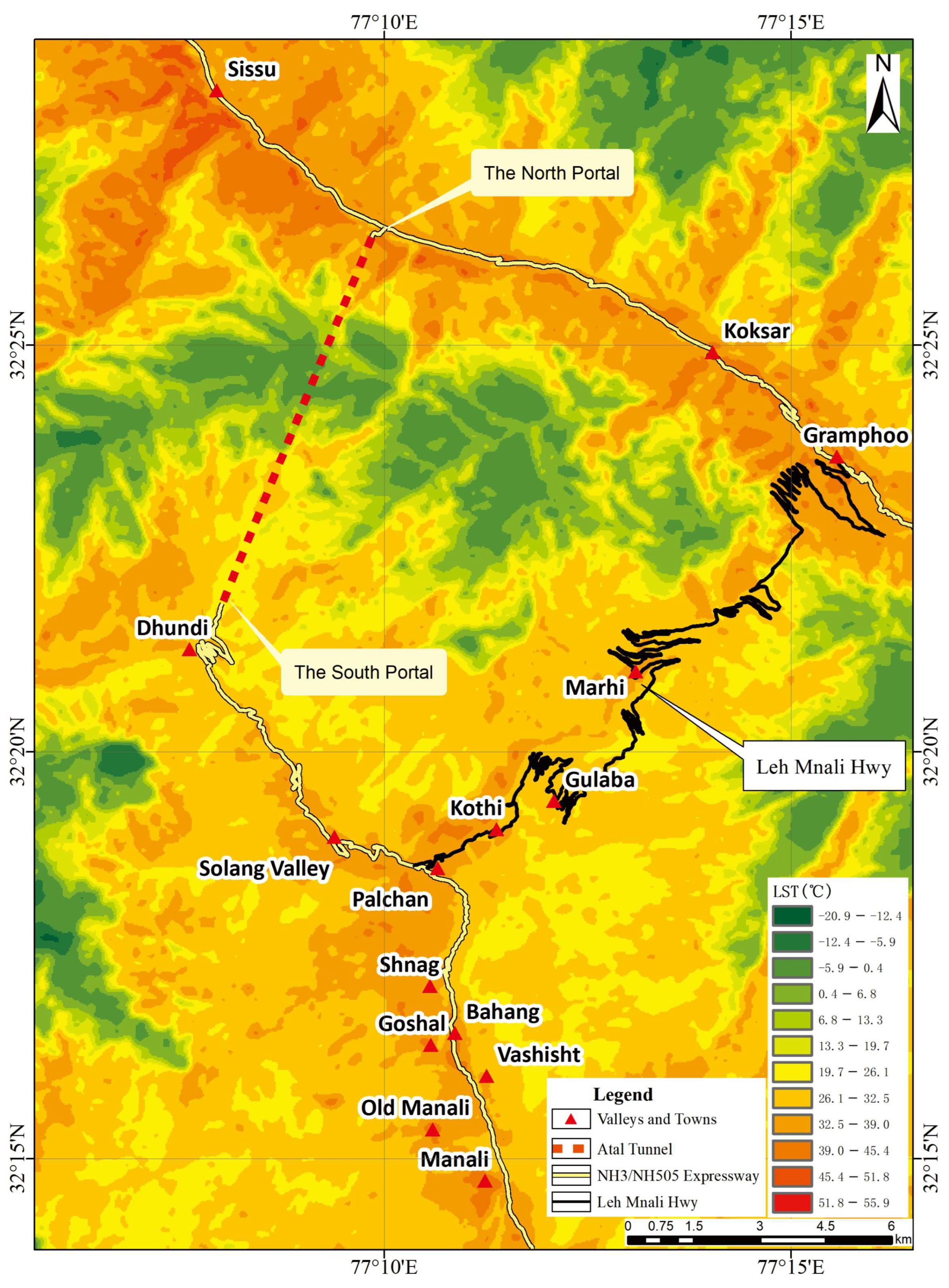
2.3.4. Land Surface Temperature

In the context of geological disaster sensitivity evaluation, the land surface temperature (LST) can be a valuable indicator due to its relationship with surface properties, vegetation cover, the moisture content, and soil conditions [62,63,64,65]. In order to obtain surface temperatures effectively, the single-window (SW) algorithm was employed to extract the surface temperature through Landsat-8 thermal infrared remote sensing (TIRS) data.

$${\mathrm{T}}_{\mathsf{\delta }}=\frac{\mathrm{a}\left(1-\mathrm{C}-\mathrm{D}\right)+\left(\mathrm{b}\left(1-\mathrm{C}-\mathrm{D}\right)+\mathrm{C}+\mathrm{D}\right){\mathrm{T}}_{\mathrm{a}}}{\mathrm{C}}$$

(5)

where a = −67.355351; b = 0.458606; C = ${\mathsf{\epsilon }}_{\delta }{\mathsf{\tau }}_{\delta }$; D = $($1 − ${\mathsf{\tau }}_{\delta }$)[1 + ${\mathsf{\tau }}_{\delta }$ (1 − ${\mathsf{\epsilon }}_{\delta }$)]; ${\mathsf{\epsilon }}_{\delta }$ is the emissivity of land surface; ${\mathsf{\tau }}_{\delta }$ is the atmospheric transmissivity; and T_a is the average action temperature. The SW algorithm formula applicable to the Landsat 8 thermal infrared band is as follows [66,67,68]:

$${\mathrm{T}}_{\mathrm{s}}=\mathsf{\gamma }[\frac{{\mathsf{\phi }}_1{\mathrm{L}}_{\mathrm{sen}}+{\mathsf{\phi }}_2}{\mathsf{\epsilon }}+{\mathsf{\phi }}_3]+\mathsf{\delta }$$

(6)

$$\mathsf{\gamma }\approx {\mathrm{T}}_{\mathrm{sen}}^2/{\mathrm{b}}_{\mathsf{\gamma }}{\mathrm{L}}_{\mathrm{sen}}$$

(7)

$$\mathsf{\delta }={\mathrm{T}}_{\mathrm{sen}} -{\mathrm{T}}_{\mathrm{sen}}^2/{\mathrm{b}}_{\mathsf{\gamma }}$$

(8)

where ε is the surface specific emissivity; γ is the parameter determined by Equation (7); δ is the parameter determined by Equation (8); for TIRS Band 10 and Band 11, b_γ is 1324 K and 1199 K, respectively; ${\mathrm{L}}_{\mathrm{sen}}$ is the spectral radiation value corresponding to the image element (W·m⁻²·sr⁻¹·μm⁻¹); ${\mathrm{T}}_{\mathrm{sen}}$ represents the brightness temperature value after conversion from the thermal infrared band; and ${\phi }_1$, ${\phi }_2$, ${\phi }_3$ are the atmospheric function parameters, respectively.

Jimenez-Mufloz et al. selected 4838 atmospheric profile data from the Global Reference Atmospheric Profile (GRAP) database and calculated the atmospheric water vapor content, atmospheric transmittance, atmospheric upward radiation, atmospheric downward radiation and other parameters by using the atmospheric radiation transmission software MODTRAN 4.0 [69,70]. The expression of the three atmospheric functions and atmospheric water vapor content for Landsat-8 was obtained by least square fitting, where ω is the atmospheric water vapor content, g/cm².

$$\left[\begin{array}{c}{\mathsf{\phi }}_1\\ {\mathsf{\phi }}_2\\ {\mathsf{\phi }}_3\end{array}\right]=\left[\begin{array}{ccc}0.04019& 0.02916& 1.01523\\ -0.38333& -1.50294& 0.20324\\ 0.00918& 1.36072& -0.27514\end{array}\right]·\left[\begin{array}{c}{\mathsf{\omega }}^2\\ \mathsf{\omega }\\ 1\end{array}\right]$$

(9)

The LST falls in between −20.9 and 55.9 °C, and we divided the results into 12 classes according to the 1/2 standard deviation. Different from the NDVI, most high values are located near the roads (Figure 7).

2.3.5. Buffer Distance

For the special case study of the Atal Tunnel, the buffer distance for roads is the distance to the central line of the tunnel. It can be considered as the factor related to human activity that is closely linked to the formation of a geological disaster [54,71]. The process of tunnel construction may destabilize the slopes on both sides of it and increase the fragmentation of rock. The roads data were converted into a grid format, and a buffer zone was divided into six classes at 200 m intervals from the central line of all roads within the study area (Figure 8a).

Rivers can cause significant erosion, especially in areas with loose soil or steep banks. A buffer distance allows for the identification of areas that might be prone to riverbank collapse or significant soil erosion, where the river’s natural course could change over time [72]. The study area encompasses two major rivers that serve as a source of water, contributing to the formation of sand. We divided the study area into six grades at intervals of 200 m from the central line of all waterways (Figure 8b).

2.4. Multicollinearity Diagnostics

In analyzing the susceptibility to geological disaster, the reliability of the predictive models is contingent upon the integrity of the underlying data. To diagnose multicollinearity within our model, we performed a multicollinearity diagnostic analysis, providing insight into the interdependencies among the predictor variables. According to the results, the maximum variance inflation factor (VIF) value of all factors is less than 10, and the minimum tolerance (Tol) value is greater than 0.1 (

Table 3. Conditioning factor categories.

Factor	TOL	VIF
slope	0.884	1.131
slope aspect	0.84	1.191
elevation	0.769	1.3
curvature	0.894	1.118
lithology	0.915	1.093
NDVI	0.921	1.086
land surface temperature (LST)	0.941	1.063
buffer distance to roads	0.785	1.275
buffer distance to rivers	0.884	1.132

), indicating that there are no severe multicollinearity issues. Therefore, these nine selected factors could be used for geological disaster susceptibility analysis.

2.5. Machine Learning Model

2.5.1. Weight of Evidence Method (WoE)

Since its initial application by Bonham-Carter in 1988 for mineral potential assessment, the WoE model has been widely adopted across various fields. Based on the statistical analysis, susceptibility mappings can be acquired as follows [73,74].

$${\mathrm{W}}_{\mathrm{i}}^{+}=\ln \frac{\mathrm{P}\left\{\mathrm{N}\right[X_i\left]\right|\mathrm{N}\left[\mathrm{L}\right]\}}{\mathrm{P}\left\{\mathrm{N}\right[X_i\left]\right|\mathrm{N}\left[\overline{\mathrm{L}}\right]\}}=\mathrm{l}\mathrm{n}\frac{\mathrm{N}(X_i\cap \mathrm{L})/\mathrm{N}\left(\mathrm{L}\right)}{\mathrm{N}(X_i\cap \overline{\mathrm{L}})/\mathrm{N}\left(\overline{\mathrm{L}}\right)},$$

(10)

$${\mathrm{W}}_{\mathrm{i}}^{-}=\ln \frac{\mathrm{P}\left\{\mathrm{N}\right[\overline{X_i}\left]\right|\mathrm{N}\left[\mathrm{L}\right]\}}{\mathrm{P}\left\{\mathrm{N}\right[\overline{X_i}\left]\right|\mathrm{N}\left[\overline{\mathrm{L}}\right]\}}=\mathrm{l}\mathrm{n}\frac{\mathrm{N}(\overline{X_i}\cap \mathrm{L})/\mathrm{N}\left(\mathrm{L}\right)}{\mathrm{N}(\overline{X_i}\cap \overline{\mathrm{L}})/\mathrm{N}\left(\overline{\mathrm{L}}\right)}.$$

(11)

In the above equation, the various stages of the distinct impact factors associated with geological disaster are identified as $X_i$, where N[$X_i$] is the number of grids contained in this stage; N[L] is the grid number with geological disaster points; N[$\overline{X_i}$] and N[$\overline{L}$] are no value, respectively; and N($X_i$∩L) is the number of grids that contain geological disasters of $X_i$.

Then, the contrasting weights can be derived through the following equation:

$${\mathrm{W}}^{+}={\mathrm{W}}_i^{+}+{\mathrm{W}}_i^{-},$$

(12)

Finally, the LSI is calculated by summing the effects, enabling the delineation of an LSZ map.

$$\mathrm{L}\mathrm{S}\mathrm{I}=\sum \mathrm{W}.$$

(13)

2.5.2. Frequency Ratio (FR)

The FR model was applied through the use of a linear combination approach, and it involves the systematic analysis of multiple parameters that influence the occurrence of geological disasters. Lee and Pradhan (2007) and Intarawichian and Dasananda (2011) successfully employed the FR model to produce a landslide susceptibility map [75,76]. The FR for each category across all data layers is calculated using the following equation:

$${\mathrm{F}\mathrm{r}}_{\mathrm{i}}=\frac{{\mathrm{N}}_{\mathrm{p}\mathrm{i}\mathrm{x}\left(\mathrm{S}\mathrm{i}\right)}/{\mathrm{N}}_{\mathrm{p}\mathrm{i}\mathrm{x}\left(\mathrm{N}\mathrm{i}\right)}}{\sum {\mathrm{N}}_{\mathrm{p}\mathrm{i}\mathrm{x}\left(\mathrm{S}\mathrm{i}\right)}/\sum {\mathrm{N}}_{\mathrm{p}\mathrm{i}\mathrm{x}\left(\mathrm{N}\mathrm{i}\right)}}$$

(14)

where ${\mathrm{N}}_{\mathrm{p}\mathrm{i}\mathrm{x}\left(\mathrm{S}\mathrm{i}\right)}$ represents the number of pixels containing a slide within each class (i); ${\mathrm{N}}_{\mathrm{p}\mathrm{i}\mathrm{x}\left(\mathrm{N}\mathrm{i}\right)}$ is the total number of pixels that fall under class (i) across the entire dataset; and $\sum {\mathrm{N}}_{\mathrm{p}\mathrm{i}\mathrm{x}\left(\mathrm{S}\mathrm{i}\right)}$ and $\sum {\mathrm{N}}_{\mathrm{p}\mathrm{i}\mathrm{x}\left(\mathrm{N}\mathrm{i}\right)}$ are both the total number.

An FR value exceeding 1 signifies a strong and positive correlation between the incidence of geological disasters within each class of the data layers and a heightened susceptibility. Conversely, a value below 1 indicates a weak and negative susceptibility.

2.5.3. Logistic Regression (LR)

The LR model is mainly employed to infer the relationship between a series of relatively independent geological environmental factors and the occurrence of geological disasters [77,78,79]. The probability of geological disasters is quantified on a scale ranging from 0 to 1, allowing for the calculation of this probability within the study area [80]. The model accommodates geological environmental factors of both a discrete and continuous nature, enabling the more precise depiction of landslide probabilities [81].

$$\mathrm{A}=\frac{\mathrm{e}\mathrm{x}\mathrm{p}\left(\mathrm{M}\right)}{1+\mathrm{e}\mathrm{x}\mathrm{p}\left(\mathrm{M}\right)}.$$

(15)

where A represents the probability of a landslide occurrence, which ranges from 0 to 1, while M refers to a linear combination.

$$\mathrm{A}=N_0+N_1{X}_1+N_2{X}_2+\cdots +N_{n}n.$$

(16)

where X₁, X₂, …, and X_n represent the variables. N₁, N₂, …, and N_n are the corresponding slope coefficients. N₀ refers to the intercept.

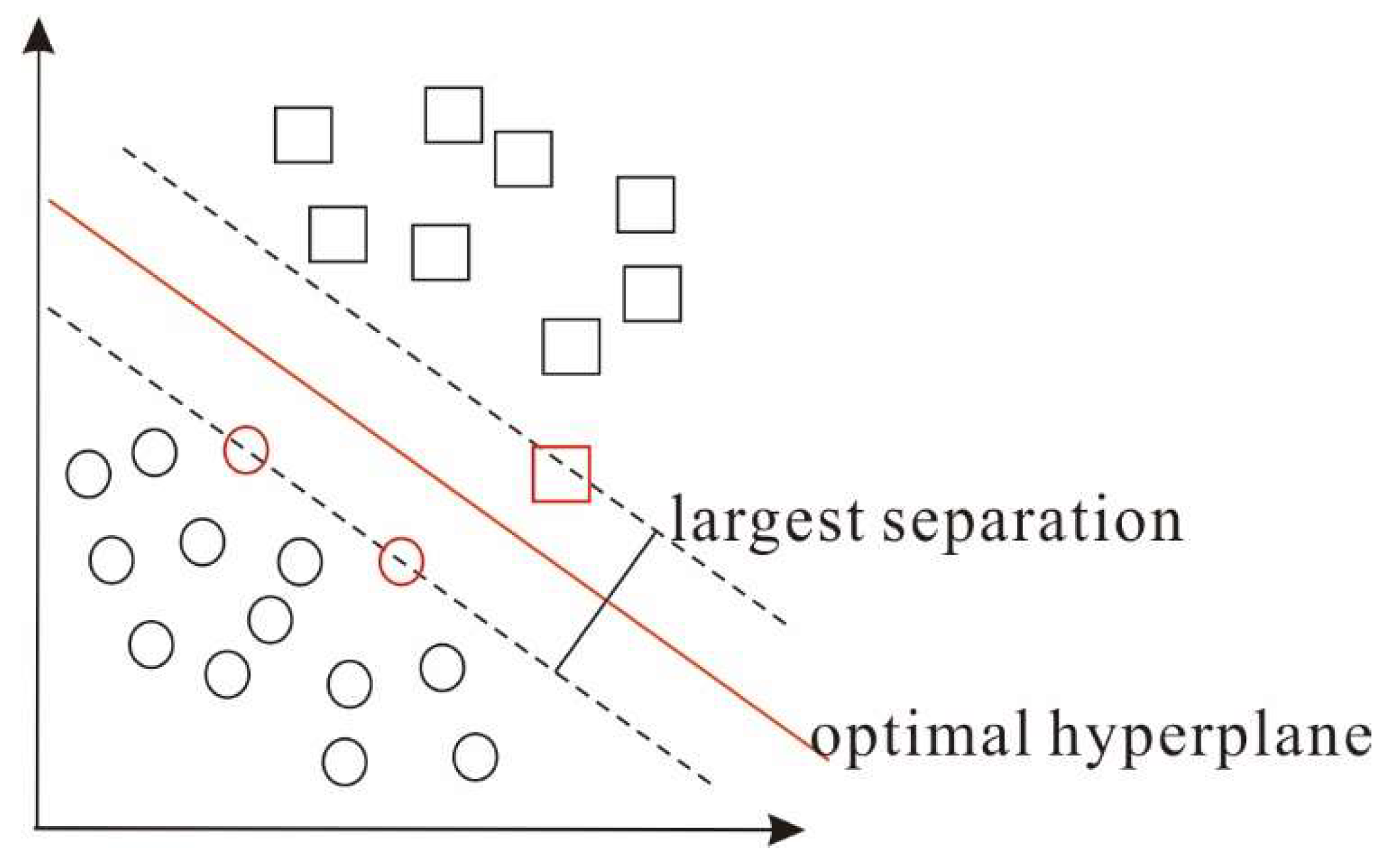
2.5.4. Support Vector Machine (SVM)

The Support Vector Machine (SVM) is a supervised machine learning algorithm that is applicable to both classification and regression tasks. The basic principle of SVM is to identify the optimal classification hyperplane within the sample space. The margin is defined as the distance between the hyperplane and the nearest data point. A larger margin equates to the greater generalization ability of the classifier, which typically results in lower error rates (Figure 9). In the field of geological disaster prediction, SVMs are useful in identifying patterns and classifying areas based on the potential for geological risk by constructing hyperplanes in a multidimensional space that separates different classes [82,83]. As a result, SVM has been extensively utilized in the analysis of geological disaster susceptibility, yielding robust outcomes.

3. Results

3.1. Analysis of Main Disaster Causing Factors

Based on the WoE and FR, the results obtained using the WoE show that the most sensitive interval of slope is 20–30°, following the slope aspect (south), elevation (2988.8–3377.4 m), curvature (<0), lithology (VII), NDVI (<0), land surface temperature (LST) (31.6–37.2), buffer distance to roads (0–200 m), and buffer distance to rivers (400–600 m). At the same time, the vast majority of results obtained by the FR are the same as those obtained by the WoE, except for the buffer distance to rivers (0–200 m) (

Table 4. Weight of factors for the WoE and FR.

Factors	Class	Class Pixel Counts	Landslide Pixel Counts	WoE	FR
Slope	0–10	105,510	2	−0.383	0.663
	10–20	259,265	2	−1.148	0.270
	20–30	447,783	22	0.087	1.717
	30–40	323,704	10	0.051	1.080
	40–50	138,219	2	−0.626	0.506
	50–60	44,438	0	0.000	0.000
	60–70	8682	0	0.000	0.000
	>70	511	0	0.000	0.000
Aspect	Flat	2687	0	0.000	0.000
	North	168,759	2	−0.800	0.414
	Northeast	147,475	2	−0.683	0.474
	East	104,053	0	0.000	0.000
	Southeast	169,348	7	0.301	1.445
	South	221,314	14	0.516	2.211
	Southwest	200,529	2	−0.944	0.349
	West	150,528	8	0.503	1.857
	Northwest	163,419	3	−0.395	0.642
Elevation	0.00%	2.63%	7.89%	15.79%	73.68%
	1673–1822.6	204	0	0.000	0.000
	1822.7–2211.3	20,482	0	0.000	0.000
	2211.4–2600	32,369	3	0.446	1.613
	2600.1–2988.7	57,668	4	0.168	1.207
	2988.8–3377.4	118,062	18	0.531	2.653
	3377.5–3766.1	120,855	11	0.320	1.584
	3766.2–4154.8	128,664	2	−1.145	0.271
	4154.9–4543.5	101,890	0	0.000	0.000
	4543.6–4932.2	54,583	0	0.000	0.000
	4932.3–5320.9	21,193	0	0.000	0.000
Curvature	−283,823,996,990–0	374,456	26	0.507	1.208
	0–237,168,001,000	286,848	12	−0.507	0.728
Lithology	Ⅰ	18,840	0	0.000	0.000
	Ⅱ	226,826	17	0.093	1.304
	Ⅲ	179,692	8	−0.174	0.775
	Ⅳ	38,801	0	0.000	0.000
	Ⅴ	5354	0	0.000	0.000
	Ⅵ	175,734	11	0.053	1.089
	Ⅶ	16,057	2	0.744	2.168
NDVI	−1–0	463,277	38	0.000	1.277
	0	98	0	0.000	0.000
	0–1	128,459	0	0.000	0.000
LST	−13.8–−12.5	226	0	0.000	0.000
	−7.0	5084	0	0.000	0.000
	−1.5	54,194	0	0.000	0.000
	4.0	41,690	0	0.000	0.000
	9.6	29,166	0	0.000	0.000
	15.1	30,398	0	0.000	0.000
	20.6	87,716	5	−0.126	0.860
	26.1	198,750	23	0.053	1.746
	31.6	99,627	6	−0.077	0.908
	37.2	23,298	4	0.882	2.590
	42.7	2984	0	0.000	0.000
	44.6	50	0	0.000	0.000
Buffer distance to roads	0–200	40,724	20	1.462	8.547
	200–400	32,672	6	1.041	3.196
	400–600	30,749	1	−0.548	0.566
	600–800	29,662	1	−0.514	0.587
	800–1000	28,721	3	0.560	1.818
	>1000	498,776	7	−0.210	0.244
Buffer distance to rivers	0–200	166,373	19	0.284	1.987
	200–400	132,260	6	−0.185	0.789
	400–600	101,909	10	0.397	1.708
	600–800	75,132	3	−0.326	0.695
	800–1000	54,903	0	0.000	0.000
	>1000	130,727	0	0.000	0.000

).

Through the LR and SVM, the factor with the largest coefficients, as determined by the LR with WoE, is the buffer distance to roads, following the LR with FR (buffer distance to roads), the SVM with WoE (buffer distance to roads) and the SVM with FR (buffer distance to roads). The results were consistent (

Table 5. The coefficient of factors, as determined by LR and SVM.

	Slope	Slope Aspect	Elevation	Curvature	Lithology	NDVI	LST	Buffer Distance to Roads	Buffer Distance to Rivers
WoE-LR	0.21	0.10	0.06	0.03	0.04	0.07	0.06	0.38	0.06
WoE-SVM	0.09	0.12	0.03	0.13	0.02	0.02	0.04	0.48	0.08
FR-LR	0.11	0.14	0.10	0.04	0.03	0.07	0.04	0.39	0.09
FR-SVM	0.28	0.04	0.19	0.04	0.04	0.02	0.04	0.31	0.04

).

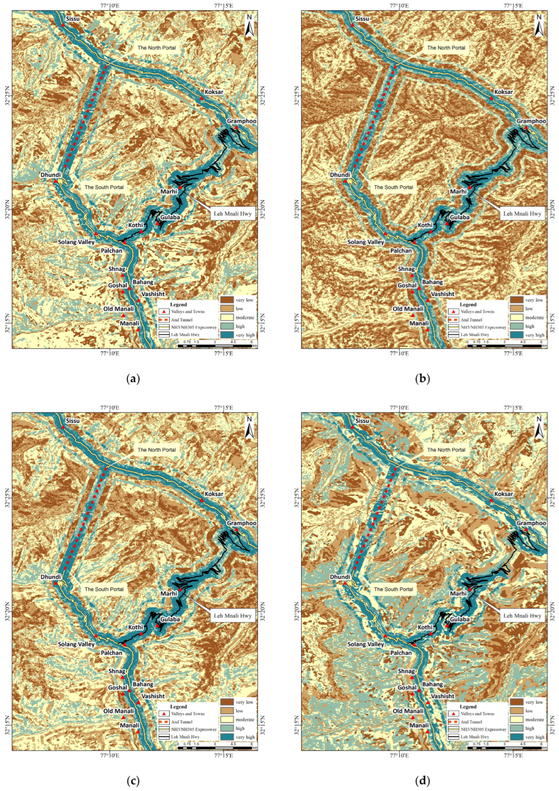
3.2. Geological Disaster Susceptibility Results

In this study, we extracted the data of eleven environmental and geological variables. The established models have been employed to predict the probability of geological disasters occurring within the study area. Pertaining to the results, the mapping outputs were categorized into five susceptibility levels: very low, low, medium, high, and very high (Figure 10,

Table 6. Comparison table of different models.

	Very Low	Low	Moderate	High	Very High
WoE-LR	0.00%	5.26%	7.89%	23.68%	63.16%
WoE-SVM	2.63%	5.26%	13.16%	18.42%	60.53%
FR-LR	0.00%	2.63%	7.89%	15.79%	73.68%
FR-SVM	2.63%	2.63%	7.89%	18.42%	68.42%

).

The result of the WoE-LR model shows that the LSI values ranged from 0 to 0.97. The proportions of disasters in each grade, from very low to very high, were 0.00%, 5.26%, 2.63%, 26.32% and 65.79%. The portions show a gradually increasing trend. And based on the WoE-SVM model, the LSI values ranged from 0 to 0.98. The proportions of disasters in each grade, from very low to very high, were 2.63%, 5.26%, 13.16%, 18.42% and 60.53%. The portions show a gradually increasing trend.

The result of the FR-LR model shows that the LSI values ranged from 0 to 0.98. The proportions of disasters in each grade, from very low to very high, were 0.00%, 2.63%, 7.89%, 15.79% and 73.68%. The portions show a gradually increasing trend. And through the FR-SVM model, it was found that the LSI values ranged from 0 to 0.97. The proportions of disasters in each grade, from very low to very high, were 2.63%, 2.63%, 7.89%, 18.42% and 68.42%. The portions show a gradually increasing trend.

3.3. ROC Curves

Geological disaster susceptibility analysis models are commonly assessed for accuracy using the receiver operating characteristic (ROC) curve and the area under the curve (AUC) metrics [84,85]. The evaluation accuracies of WoE-LR, WoE-SVM, FR-LR and FR-SVM are 90.7%, 88.2%, 90.2% and 88.2%, respectively. In the meantime, the AUC values are 0.907, 0.902, 0.882 and 0.882, respectively. The results reveal which method is more suitable for working in high-altitude areas. The accuracy rate obtained by the five calculation models exceeded 85%, and the WoE-LR model achieved the highest accuracy rate (Figure 11).

4. Discussion

Based on remote sensing images and the calculate models, this study evaluates geological disaster susceptibility for the Atal Tunnel region. When using the WoE and FR model, the results are consistent; 20–30° is the most sensitive interval of slope, because when the slope is under 20°, the rock and soil are stable. Conversely, when the slope is above 30°, the rock and soil are unable to attach. Similarly, the south of the aspect and the 2988.8–3377.4 m elevation accept strong weathering. A concave-shaped slope can accept more wind erosion, the more easily broken lithology is VII, and exposed areas have the weakest resistance to weathering. The high temperature catalyzes the process of weathering, and the presence of roads and rivers further causes rock fragmentation due to their power. When the environment combines all the above situations, landslides are extremely easy to generate.

In order to find the more accurate landslide susceptibility mapping, this paper chose FR and SVM to participate in hybrid model operations. After comparing the table of different models, all portions show a gradually increasing trend from very low to very high. The result shows that all hybrid models have good applicability. Among them, the WoE-LR is the most applicable for the study area, with a probability of 92.11 between high and very high. Through the results, despite utilizing the same dataset for disasters and environmental variables in each model, significant differences were observed in the evaluations of susceptibility. The four models used above each have advantages and disadvantages according to the different algorithm operations. The analysis of the ROC curve indicates that the accuracy of the four models exceeds 85%, and that WoE-LR is the best among them. In the susceptibility evaluation of the Atal Tunnel, the distance to roads was found to be the most important factor. According to the results of the four models, the areas with many geological disasters in the study area are mainly distributed along the roads. What is more, there are also some other disaster-causing factors, such as a higher LST.

With advancements in information technology, an increasing number of machine learning models are being employed to analyze geological disaster susceptibility. Many experts have invested in deep learning models such as the Artificial Neural Network (ANN), Convolutional Neural Network (CNN), and Recurrent Neural Network (RNN) for the study of land hazard vulnerability [86,87]. However, there are also some disadvantages, such as the requirement of an extensive number of parameters; unobservable learning processes; and difficulties interpreting the classification results in the models. Because of the complex and challenging terrain along the Atal Tunnel, it is very challenging to carry out conventional large-area ground surveys. The above analysis demonstrates that evaluating the susceptibility of the tunnel area to geological disasters is feasible. The multi-source remote sensing data obtained with high spatial and spectral resolutions have played important roles in the study area. Integrating the mechanism of spatial information acquisition and analysis, remote sensing technology can provide essential and basic information such as the spatial positioning of disaster-causing factors, which is fundamental to tunnel construction in challenging areas such as the Tibetan Plateau. Furthermore, a more objective differentiation among various models has been observed, facilitating the derivation of superior model combinations. Incorporating the logical regression model enables the calculation of coefficients for each contributing factor, thereby accentuating their distinct roles in the final computation of LSI, leading to more precise and robust evaluation outcomes. For areas prone to significant geological disasters, the selection of tunnel routes should prioritize disaster avoidance, followed by rapid transit through areas of low or no risk; this is achieved by a thorough analysis of the distribution patterns and environmental variables of geological disasters. Nevertheless, owing to the multitude of variables that can influence outcomes, there also exists a substantial potential for serious misguidance if any factors are not meticulously taken into account. What is more, on account of the special location, we did not perform a geological investigation, so the results cannot be verified; there is still some uncertainty in different models, which are perhaps not suitable for the cities and plains. In future research, we will focus on the full potential of multi-source data and delve into the intrinsic relationships among various factors. Additionally, we will be devoted to applying the most effective monitoring techniques to assess the stability of geological disasters using multi-source monitoring data, and this effort will significantly contribute to the site selection processes as well as guarantee the safety of tunnel constructions.

5. Conclusions

Our study utilized GIS-based machine learning analysis technology to assess the geological disaster susceptibility of the Atal Tunnel study area. Increasing numbers of tunnels similar to the Atal Tunnel will be constructed in this area in the future. The significance of internal and external dynamic geological processes cannot be overstated, given the multitude of complex geological conditions such as a large burial depth, active faults, and high altitudes. The method employed in this study markedly reduces the need for the financial and personnel investments typically required for geological investigations. By relying on quantifiable data and robust algorithms, these models minimize the influence of subjective human factors that may introduce bias or inconsistency into the evaluation process. At the same time, they enable the following key findings to be obtained:

(1)

It is feasible and effective to apply the hybrid model to evaluate the local areas of tunnels with strong human activity.

(2)

Many factors have contributed to the occurrence of landslides, so more factors should be considered in landslide susceptibility mapping. Among the factors chosen in this paper, the buffer distance to roads serves as the most critical factor in the evaluation of tunnel geological disaster susceptibility.

(3)

By comparing the efficacy of the four hybrid models, it is clear that the WOE-LR model is more suitable for the study area, achieving a superior performance, with a 92.11% identification rate for areas at high and very high risk. Meanwhile, the WOE-LR model is also proven to be particularly effective for geological risk assessment in the Atal Tunnel, with an AUC value of 0.907 and an accuracy rate of 90.7%.

The application of GIS-based machine learning analysis in this study not only sets a precedent for future geological assessments in similar regions, but also contributes to the broader field of sustainable infrastructure development. By providing a method that is both scientifically rigorous and economically feasible, this research paves the way for safer and more efficient infrastructure projects in geologically complex areas like the Tibetan Plateau. Moreover, the scalability of machine learning models means that as more data become available, these models can be refined and adapted to new challenges, increasing their accuracy and applicability. In the future, we will continue to integrate additional machine learning models to further refine the accuracy of our assessments. This initiative will help advance the field of geological disaster evaluation. This iterative process of learning and adaptation will further enhance our ability to predict and mitigate geological disasters, safeguarding both human lives and investments. Additionally, the integration of GIS-based machine learning analysis with other emerging technologies, such as satellite imagery analysis and drone surveillance, could provide a more comprehensive understanding of geological disasters. However, there are also some certain limitations in this paper. The factors chosen for research are not comprehensive enough, and detailed geological survey work was not carried out. These caused deviations between the results and the actual situation. Therefore, in future research, this article will collect more detailed relevant factors and workspace conditions in order to obtain more accurate geological disaster susceptibility mapping for tunnel safety protection.

References

1. Wu, F.; Jin, H.; Shang, Y. Underground pipeline deformation prediction around urban rail transit tunnel engineering. Chin. J. Rock Mech. Eng. 2013, 32, 3592–3601. [Google Scholar]
2. Xia, Y.-X.; Ye, F.; Zhao, F.; Wang, L.Z. Construction quality management of highway tunnel engineering. J. Chang. Univ. 2007, 27, 63–66. [Google Scholar]
3. Zhou, W.; Qin, H.; Qiu, J.; Fan, H.; Lai, J.; Wang, K.; Wang, L. Building information modelling review with potential applications in tunnel engineering of China. R. Soc. Open Sci. 2017, 4, 170174. [Google Scholar] [CrossRef] [PubMed]
4. Shan, C.X.; Shi, L.Z.; Jian, P.C. The Application of Fuzzy-Analytic Evaluation in Geological Disaster Assessment for Tunnel Construction. Chin. J. Undergr. Space Eng. 2013, 9, 946–953. [Google Scholar]
5. Xu, W.; Kang, Y.; Chen, L.; Wang, L.; Qin, C.; Zhang, L.; Liang, D.; Wu, C.; Zhang, W. Dynamic assessment of slope stability based on multi-source monitoring data and ensemble learning approaches: A case study of Jiuxianping landslide. Geol. J. 2023, 58, 2353–2371. [Google Scholar] [CrossRef]
6. Chen, Z.; Chang, R.; Guo, H.; Pei, X.; Zhao, W.; Yu, Z.; Zou, L. Prediction of potential geothermal disaster areas along the Yunnan–Tibet railway project. Remote Sens. 2022, 14, 3036. [Google Scholar] [CrossRef]
7. Agarwal, K.K.; Shah, R.A.; Achyuthan, H.; Singh, D.S.; Srivastava, S.; Khan, I. Neotectonic activity from Karewa Sediments, Kashmir Himalaya, India. Geotectonics 2018, 52, 88–99. [Google Scholar] [CrossRef]
8. Nazir, S.; Simnani, S.; Sahoo, B.K.; Mishra, R.; Sharma, T.; Masood, S. Monitoring geothermal springs and groundwater of Pir Panjal, Jammu and Kashmir, for radon contamination. J. Radioanal. Nucl. Chem. 2020, 326, 1915–1923. [Google Scholar] [CrossRef]
9. Ahmad, S.; Bhat, M.I. Tectonic geomorphology of the Rambiara basin SW Kashmir Valley reveals emergent out-of-sequence active fault system. Himal. Geol. 2012, 33, 162–172. [Google Scholar]
10. Akram, M.S.; Mirza, K.; Zeeshan, M.; Ali, I. Correlation of tectonics with geologic lineaments interpreted from remote sensing data for Kandiah Valley, Khyber-Pakhtunkhwa, Pakistan. J. Geol. Soc. India 2019, 93, 607–613. [Google Scholar] [CrossRef]
11. Van Westen, C.J.; Castellanos, E.; Kuriakose, S.L. Spatial data for landslide susceptibility, hazard, and vulnerability assessment: An overview. Eng. Geol. 2008, 102, 112–131. [Google Scholar] [CrossRef]
12. Karim, Z.; Hadji, R.; Hamed, Y. GIS-based approaches for the landslide susceptibility prediction in Setif Region (NE Algeria). Geotech. Geol. Eng. 2019, 37, 359–374. [Google Scholar]
13. Pradhan, B.; Lee, S. Delineation of landslide hazard areas on Penang Island, Malaysia, by using frequency ratio, logistic regression, and artificial neural network models. Environ. Earth Sci. 2010, 60, 1037–1054. [Google Scholar] [CrossRef]
14. Anis, Z.; Wissem, G.; Riheb, H.; Biswajeet, P.; Essghaier, G.M. Effects of clay properties in the landslides genesis in flysch massif: Case study of Aïn Draham, North Western Tunisia. J. Afr. Earth Sci. 2019, 151, 146–152. [Google Scholar] [CrossRef]
15. Hadji, R.; Raïs, K.; Gadri, L.; Chouabi, A.; Hamed, Y. Slope failures characteristics and slope movement susceptibility assessment using GIS in a medium scale: A case study from Ouled Driss and Machroha municipalities, Northeastern of Algeria. Arab. J. Sci. Eng. 2017, 42, 281–300. [Google Scholar] [CrossRef]
16. Dhakal, A.; Amada, T.; Aniya, M. Landslide hazard mapping and its evaluation using GIS: An investigation of sampling schemes for a grid-cell based quantitative method. Remote Sens. 2000, 66, 981–989. [Google Scholar]
17. Kahal, A.Y.; Abdelrahman, K.; Alfaifi, H.J.; Yahya, M.M. Landslide hazard assessment of the Neom promising city, Northwestern Saudi Arabia: An Integrated Approach. J. King Saud Univ. Sci. 2021, 33, 101279. [Google Scholar] [CrossRef]
18. Lee, C.F.; Li, J.; Xu, Z.W.; Dai, F.C. Assessment of landslide susceptibility on the natural terrain of Lantau Island. Hong Kong. Environ. Geol. 2001, 40, 381–391. [Google Scholar] [CrossRef]
19. Manchar, N.; Benabbas, C.; Hadji, R.; Bouaicha, F.; Grecu, F. Landslide Susceptibility Assessment in Constantine Region Algeria by Means of Statistical Models. Stud. Geotech. Mech. 2018, 40, 208–219. [Google Scholar] [CrossRef]
20. Chang, L.; Hanssen, R.F. Detection of permafrost sensitivity of the Qinghai–Tibet railway using satellite radar interferometry. Int. J. Remote Sens. 2015, 36, 691–700. [Google Scholar] [CrossRef]
21. Ma, X.; Yao, Y.; Zhang, B.; Yang, M.; Liu, H. Improving the accuracy and spatial resolution of precipitable water vapor dataset using a neural network-based downscaling method. Atmos. Environ. 2022, 269, 118850. [Google Scholar] [CrossRef]
22. Beselly, S.M.; van der Wegen, M.; Grueters, U.; Reyns, J.; Dijkstra, J.; Roelvink, D. Eleven years of Mangrove-Mudflat dynamics on the mud volcano-induced prograding delta in East Java, Indonesia: Integrating UAV and satellite imagery. Remote Sens. 2021, 13, 1084. [Google Scholar] [CrossRef]
23. Csajbók, J.; Buday-Bódi, E.; Nagy, A.; Fehér, Z.Z.; Tamás, A.; Virág, I.C.; Bojtor, C.; Forgács, F.; Vad, A.M.; Kutasy, E. Multispectral analysis of small plots based on field and remote sensing surveys-A comparative evaluation. Sustainability 2022, 14, 3339. [Google Scholar] [CrossRef]
24. Ni, J.; Wu, T.; Zhu, X.; Hu, G.; Zou, D.; Wu, X.; Li, R.; Xie, C.; Qiao, Y.; Pang, Q.; et al. Simulation of the present and future projection of permafrost on the Qinghai-Tibet Plateau with statistical and machine learning models. J. Geophys. Res. Atmos. 2024, 3, e2020JD033402. [Google Scholar] [CrossRef]
25. Ozdemir, A.; Altural, T. A comparative study of frequency ratio, weights of evidence and logistic regression methods for landslide susceptibility mapping: Sultan Mountains, SW Turkey. J. Asian Earth Sci. 2013, 64, 180–197. [Google Scholar] [CrossRef]
26. Bassam, B.F.A. GIS predictive model for producing hydrothermal gold potential map using Weights of Evidence approach in Gengma region, Sanjiang district, China. J. China Univ. Geosci. 2003, 14, 283–292. [Google Scholar]
27. Zhao, Z.; Liu, Z.Y.; Xu, C. Slope unit-based landslide susceptibility mapping using certainty factor (cf), support vector machine (svm), random forest (rf), cf-svm and cf-rf models. Front. Earth Sci. 2021, 9, 589–630. [Google Scholar] [CrossRef]
28. Gomes, R.A.T.; Guimarães, R.F.; Carvalho Júnior, O.A.D.; Fernandes, N.F.; Amaral Júnior, E.V.D. Combining spatial models for shallow landslides and debris-flows prediction. Remote Sens. 2013, 5, 2219–2237. [Google Scholar] [CrossRef]
29. Hong, H.; Chen, W.; Xu, C.; Youssef, A.M.; Pradhan, B.; Tien Bui, D. Rainfall-induced landslide susceptibility assessment at the Chongren area (China) using frequency ratio, certainty factor, and index of entropy. Geocarto Int. 2016, 32, 139–154. [Google Scholar] [CrossRef]
30. Meghanadh, D.; Maurya, V.K.; Tiwari, A.; Dwivedi, R. A multi-criteria landslide susceptibility mapping using deep multi-layer perceptron network: A case study of srinagar-rudraprayag region (India). Adv. Space Res. Off. J. Comm. Space Res. 2022, 69, 1883–1893. [Google Scholar] [CrossRef]
31. Zhang, L.; Yuan, S. Logistic Regression Analysis on the correlation between physical diseases and life events and depression in the Elderly. Med. Plant 2023, 14, 92–93. [Google Scholar]
32. Zhang, T.Y.; Fu, Q.; Li, C.; Liu, F.; Wang, H.; Han, L.; Quevedo, R.P.; Chen, T.; Lei, N. Modeling landslide susceptibility using data mining techniques of kernel logistic regression, fuzzy unordered rule induction algorithm, SysFor and random forest. Nat. Hazards 2022, 114, 3327–3358. [Google Scholar] [CrossRef]
33. Joachims, T. Making Large-Scale SVM Learning Practical. Tech. Rep. 1998, 8, 499–526. [Google Scholar]
34. Lee, Y.J.; Mangasarian, O.L. SSVM: A Smooth Support Vector Machine for Classification. Comput. Optim. Appl. 2001, 20, 5–22. [Google Scholar] [CrossRef]
35. Mao, Y.X.; Zheng, M.Z.; Wang, T.Q.; Duan, M. A new mooring failure detection approach based on hybrid LSTM-SVM model for semi-submersible platform. Ocean Eng. 2023, 275, 114–161. [Google Scholar] [CrossRef]
36. Wang, D.; Liu, S.; Zhang, C.; Xu, M.; Yang, J.; Yasir, M.; Wan, J. An improved semantic segmentation model based on SVM for marine oil spill detection using SAR image. Mar. Pollut. Bull. 2023, 6, 192. [Google Scholar] [CrossRef] [PubMed]
37. Lv, Z.Y. Study on Early Triassic Conodont Biostratigraphy in Enshi and Kashmir, Hubei Province. Ph.D. Thesis, China University of Geosciences, Wuhan, China, 2018. [Google Scholar]
38. Wakaru, S.N.; Dahl, B.L. Geology in and around Kashmiri Himalayan Kshtwa and Doda districts. Yunnan Geol. 1997, S1, 6–17. [Google Scholar]
39. Avouac, J.P.; Ayoub, F.; Leprince, S.; Konca, O.; Helmberger, D.V. The 2005, Mw 7.6 Kashmir earthquake: Sub-pixel correlation of ASTER images and seismic waveforms analysis. Earth Planet. Sci. Lett. 2006, 249, 514–528. [Google Scholar] [CrossRef]
40. Schiffman, C.; Bali, B.S.; Szeliga, W.; Bilham, R. Seismic slip deficit in the Kashmir Himalaya from GPS observations. Geophys. Res. Lett. 2013, 40, 5642–5645. [Google Scholar] [CrossRef]
41. Ali, S.A.; Ali, U. Litho-Structural mapping of sind catchment (Kashmir Basin), NW Himalaya, using remote sensing & GIS techniques. Int. J. Sci. Res. 2015, 4, 1325–1330. [Google Scholar]
42. Dar, G.H.; Malik, A.H.; Khuroo, A.A. A contribution to the flora of Rajouri and Poonch districts in the Pir Panjal Himalaya (Jammu & Kashmir), India. Check List 2014, 10, 317–328. [Google Scholar]
43. Ahmad, S.; Bhat, M.I.; Madden, C.; Bali, B.S. Geomorphic analysis reveals active tectonic deformation on the eastern flank of the Pir Panjal Range, Kashmir Valley, India. Arab. J. Geosci. 2014, 7, 2225–2235. [Google Scholar] [CrossRef]
44. Kaila, K.L.; Tripathi, K.M.; Dixit, M.M. Crustal structure along Wular Lake-Gulmarg-Naoshera profile across Pir Panjal Range of the Himalayas from deep seismic soundings. J. Geol. Soc. India 1984, 25, 706–719. [Google Scholar]
45. Bhat, M.S. Spring water quality and human health in foothill settlements of Pir Panjal Range in Anantnag and Kulgam Districts of Jammu and Kashmir. In Environmental Deterioration and Human Health: Natural and Anthropogenic Determinants; Rather, G.M., Rafiq, A., Hajam, M., Bhat, S., Kanth, T.A., Eds.; Springer: Berlin/Heidelberg, Germany, 2014. [Google Scholar]
46. Saxena, S.A. Atal Tunnel. Indian Railw. 2020, 9, 52–55. [Google Scholar]
47. Aakash, V. Excavation Method Implemented in Atal (Rohtang) Tunnel-a Case Study. Tech. Pap. 2021, 6, 1065–1068. [Google Scholar] [CrossRef]
48. Sharma, K.K. Study of roof collapse in Rohtang Tunnel during construction. J. Rock Mech. Tunn. Technol. 2016, 22, 11–20. [Google Scholar]
49. Kumar, A. Hydrological conditions of River Beas and its fish fauna in Kullu Valley. Himachal Pradesh, India. Environ. Conserv. J. 2010, 11, 7–10. [Google Scholar] [CrossRef]
50. Kumar, V.; Sharma, A.; Thukral, A.; Bhardwaj, R. Assessment of soil enzyme activities based on sediment samples from the Beas river bed, India using multivariate techniques. Malays. J. Soil Sci. 2016, 20, 135–145. [Google Scholar]
51. Sharma, L.P.; Patel, N.; Ghose, M.K.; Debnath, P. Development and application of Shannon’s entropy integrated information value model for landslide susceptibility assessment and zonation in Sikkim Himalayas in India. Nat. Hazards 2014, 75, 1555–1576. [Google Scholar] [CrossRef]
52. Zahri, F.; Boukelloul, M.; Hadji, R.; Talhi, K. Slope Stability Analysis in Open Pit Mines of Jebel Gustar Career, Ne Algeria—A Multi-Steps Approach. Min. Sci. 2016, 23, 137–146. [Google Scholar]
53. Basharat, M.; Shah, H.R.; Hameed, N. Landslide susceptibility mapping using GIS and weighted overlay method: A case study from NW Himalayas, Pakistan. Arab. J. Geosci. 2016, 9, 292. [Google Scholar] [CrossRef]
54. Chen, W.; Pourghasemi, H.R.; Zhao, Z. A gis-based comparative study of dempster-shafer, logistic regression and artificial neural network models for landslide susceptibility mapping. Geocarto Int. 2017, 32, 367–385. [Google Scholar] [CrossRef]
55. Tang, D.M.; Zeng, J.Q. Discussion on testing and interpretation for possion’s ratio. Chin. J. Rock Mech. Eng. 2001, S1, 1772–1775. [Google Scholar]
56. Li, Y.H.; Wu, Q.J.; An, Z.H.; Tian, X.B.; Zeng, R.S.; Zhang, R.Q.; Li, H.G. The passion ratio and crustal structure across the NE Tibetan Plateau determined from receiver functions. Chin. J. Geophys. 2006, 5, 1359–1368. [Google Scholar]
57. Xie, R.C.; Zhou, W.; Yang, Z.B.; Shan, Y.M.; Zhou, Q.M.; Zhang, S.J. Testing characteristics and log interpretation of rock’s poisson ratio under simulating formation condition. Well Logging Technol. 2011, 35, 218–223. [Google Scholar]
58. Fensholt, R.; Rasmussen, K.; Nielsen, T.T.; Mbow, C. Evaluation of earth observation based long term vegetation trends—Intercomparing NDVI time series trend analysis consistency of Sahel from AVHRR GIMMS, Terra MODIS and SPOT VGT data. Remote Sens. Environ. 2009, 113, 1886–1898. [Google Scholar] [CrossRef]
59. Guo, J.T.; Wang, K.B.; Wang, T.J.; Bai, N.; Zhang, H.; Cao, Y.; Liu, H. Spatiotemporal variation of vegetation NDVI and its climatic driving forces in Global Land Surface. Pol. J. Environ. Stud. 2022, 31, 3541–3549. [Google Scholar] [CrossRef]
60. Caruso, G.; Palai, G.; Tozzini, L.; D’Onofrio, C.; Gucci, R. The role of LAI and leaf chlorophyll on NDVI estimated by UAV in grapevine canopies. Sci. Hortic. 2023, 322, 112398. [Google Scholar] [CrossRef]
61. Davis, Z.; Nesbitt, L.; Guhn, M.; Bosch, M.v.D. Assessing changes in urban vegetation using Normalised Difference Vegetation Index (NDVI) for epidemiological studies. Urban For. Urban Green. 2023, 88, 128080. [Google Scholar] [CrossRef]
62. Harod, R.; Eswar, R.; Bhattacharya, B.K. Effect of surface emissivity and retrieval algorithms on the accuracy of Land Surface Temperature retrieved from Landsat data. Remote Sens. Lett. 2021, 12, 983–993. [Google Scholar] [CrossRef]
63. Harvey, M.C.; Rowland, J.V.; Luketina, K.M. Drone with thermal infrared camera provides high resolution georeferenced imagery of the Waikite geothermal area, New Zealand. J. Volcanol. Geotherm. Res. 2016, 325, 61–69. [Google Scholar] [CrossRef]
64. Bian, Y.; Yang, Y.P.; Li, M.; He, X.; Tang, H.; Sun, A.; Ju, X. Application of thermal infrared remote sensing techniques in geothermal resources surveying. China Min. Mag. 2021, 30, 5. [Google Scholar]
65. Fu, P.; Weng, Q. A time series analysis of urbanization induced land use and land cover change and its impact on land surface temperature with Landsat imagery. Remote Sens. Environ. 2016, 175, 205–214. [Google Scholar] [CrossRef]
66. Nishar, A.; Richards, S.; Breen, D.; Robertson, J.; Breen, B. Thermal infrared imaging of geothermal environments and by an unmanned aerial vehicle (UAV): A case study of the Wairakei–Tauhara geothermal field, Taupo, New Zealand. Renew. Energy 2016, 86, 1256–1264. [Google Scholar] [CrossRef]
67. Sobrino, J.A.; Jiménez-Muñoz, J.C. Minimum configuration of thermal infrared bands for land surface temperature and emissivity estimation in the context of potential future missions. Remote Sens. Environ. Interdiscip. J. 2014, 148, 158–167. [Google Scholar] [CrossRef]
68. Sobrino, J.A.; Jiménez-Muñoz, J.C.; Paolini, L. Land surface temperature retrieval from LANDSAT TM 5. Remote Sens. Environ. Interdiscip. J. 2014, 90, 434–440. [Google Scholar] [CrossRef]
69. Jiménez-Muñoz, J.C.; Sobrino, J.A.; Gillespie, A.R. Surface emissivity retrieval from airborne hyperspectral scanner data: Insights on atmospheric correction and noise removal. IEEE Geosci. Remote Sens. Lett. 2012, 9, 180–184. [Google Scholar] [CrossRef]
70. Chen, L.; Bai, Z.P.; Su, D.; You, Y.; Li, H.; Liu, Q. Application of land use regression to simulate ambient air PM10 and NO2 concentration in Tianjin City. China Environ. Ence 2009, 29, 685–691. [Google Scholar]
71. Usui, H.; Asami, Y. Method for determining buffer distance to judging adjacency of lots to roads. J. Archit. Plan. 2010, 75, 1175–1180. [Google Scholar] [CrossRef]
72. Marioti, J.; Bertol, I.; Ramos, J.C.; Werner, R.D.S.; Padilha, J.; Bandeira, D.H. Water erosion from no-tillage corn and soybean sown along and perpendicularly to the contour lines, compared with bare fallow soil. Rev. Bras. Ciência Solo 2013, 37, 1361–1371. [Google Scholar] [CrossRef]
73. Achour, Y.; Pourghasemi, H.R. How do machine learning techniques help in increasing accuracy of landslide susceptibility maps? Geosci. Front. 2019, 11, 871–883. [Google Scholar] [CrossRef]
74. Xiao, T.; Yin, K.; Yao, T.; Liu, S. Spatial prediction of landslide susceptibility using GIS-based statistical and machine learning models in Wanzhou County, Three Gorges Reservoir. China Acta Geochim. 2019, 38, 654–669. [Google Scholar] [CrossRef]
75. Lee, S.; Pradhan, B. Landslide hazard mapping at Selangor, Malaysia using frequency ratio and logistic regression models. Landslides 2007, 4, 33–41. [Google Scholar] [CrossRef]
76. Intarawichian, N.; Dasananda, S. Frequency ratio model based landslide susceptibility mapping in lower Mae Chaem watershed. N. Thail. Environ. Geol. 2011, 64, 2271–2285. [Google Scholar]
77. Wu, Z.; Wu, Y.; Yang, Y.; Chen, F.; Zhang, N.; Ke, Y.; Li, W. A comparative study on the landslide susceptibility mapping using logistic regression and statistical index models. Arab. J. Geosci. 2017, 10, 187. [Google Scholar] [CrossRef]
78. Lombardo, L.; Mai, P.M. Presenting logistic regression-based landslide susceptibility results. Eng. Geol. 2018, 244, 14–24. [Google Scholar] [CrossRef]
79. Yang, J.; Song, C.; Yang, Y.; Xu, C.; Guo, F.; Xie, L. New method for landslide susceptibility mapping supported by spatial logistic regression and GeoDetector: A case study of Duwen Highway Basin, Sichuan Province, China. Geomorphology 2019, 324, 62–71. [Google Scholar] [CrossRef]
80. Mahdadi, F.; Boumezbeur, A.; Hadji, R.; Kanungo, D.P.; Zahri, F. GIS-based landslide susceptibility assessment using statistical models: A case study from Souk Ahras province, NE Algeria. Arab. J. Geosci. 2018, 11, 476. [Google Scholar] [CrossRef]
81. Daya, S.B.; Cheng, Q.; Agterberg, F. Handbook of Mathematical Geosciences; Springer International Publishing: Cham, Switzerland, 2018. [Google Scholar]
82. Tien Bui, D.; Tuan, T.A.; Klempe, H.; Pradhan, B.; Revhaug, I. Spatial prediction models for shallow landslide hazards: A comparative assessment of the efficacy of support vector machines, artificial neural networks, kernel logistic regression, and logistic model tree. Landslides 2016, 13, 361–378. [Google Scholar] [CrossRef]
83. Hong, H.; Liu, J.; Zhu, A.-X.; Shahabi, H.; Pham, B.T.; Chen, W.; Pradhan, B.; Bui, D.T. A novel hybrid integration model using support vector machines and random subspace for weather-triggered landslide susceptibility assessment in the Wuning area (China). Environ. Earth Sci. 2017, 76, 652. [Google Scholar] [CrossRef]
84. Robin, X.; Turck, N.; Hainard, A.; Tiberti, N.; Lisacek, F.; Sanchez, J.-C.; Müller, M. pROC: An open-source package for R and S+ to analyze and compare ROC curves. BMC Bioinform. 2011, 12, 77. [Google Scholar] [CrossRef] [PubMed]
85. Lobo, J.M.; Jiménez-Valverde, A.; Real, R. AUC: A misleading measure of the performance of predictive distribution models. Glob. Ecol. Biogeogr. 2010, 17, 145–151. [Google Scholar] [CrossRef]
86. Wang, J.; Yang, Y.; Mao, J.H.; Huang, Z.; Huang, C.; Xu, W. CNN-RNN: A Unified Framework for Multi-label Image Classification. In Proceedings of the IEEE Conference on Computer Vision and Pattern Recognition, Las Vegas, NV, USA, 27–30 June 2016; pp. 2285–2294. [Google Scholar]
87. Purnamasari, P.D.; Taqiyuddin, M.; Ratna, A.A.P. Performance comparison of text-based sentiment analysis using recurrent neural network and convolutional neural network. In Proceedings of the 3rd International Conference on Communication and Information Processing, Tokyo, Japan, 24–27 November 2017. [Google Scholar]
Figure 1. Location of the Atal Tunnel (Landsat 8 image).
Sustainability 16 04604 g001
Figure 2. Stratigraphic division of the Atal Tunnel.
Sustainability 16 04604 g002
Figure 3. Geological disaster distribution.
Sustainability 16 04604 g003
Figure 4. Calculation according to DEM: (a) Slope; (b) Aspect; (c) Elevation; (d) Curvature.
Sustainability 16 04604 g004aSustainability 16 04604 g004b
Figure 5. Hardness classification.
Sustainability 16 04604 g005
Figure 6. NDVI of the study area.
Sustainability 16 04604 g006
Figure 7. LST of the study area.
Sustainability 16 04604 g007
Figure 8. Distance to selected variables: (a) Distance to the roads; (b) Distance to the rivers.
Sustainability 16 04604 g008
Figure 9. Principle diagram of SVM. (The squares and circles represent two types of samples respectively, and the red ones mean the point on the optimal hyperplane).
Sustainability 16 04604 g009
Figure 10. Susceptibility mapping by the models: (a) WoE-LR; (b) WoE-SVM; (c) FR-LR; (d) FR-SVM.
Sustainability 16 04604 g010
Figure 11. ROC curves.
Sustainability 16 04604 g011