Abstract
The further promotion of cycling is a key component for each city to reach its sustainability goals. To make decisions to improve comfort or safety for cyclists, the amount of motorized traffic should be taken into account. Therefore, traffic data play a crucial role not only in the construction of roads but also in cycling planning. This data source provides insights essential for road infrastructure development and optimizing various modes of transportation, such as bike paths. However, processing municipal traffic data becomes a challenge when stationary traffic-counting stations lack geo-referencing in relational databases. In this case, the locations of traffic counters are solely displayed on a PDF-based site map without inherent geo-referencing, and the geo-coordinates are not stored in any relational database. The absence of geo-references poses a significant hurdle for traffic-planning experts in decision-making processes. Hence, this study aims to address this issue by finding a suitable approach to extract the geo-coordinates from the site maps. Several potential solutions are discussed and compared in terms of time dimension, usability, extensibility, error treatment and the accuracy of results. Leveraging the open-source tool QGIS, geo-coordinates may be successfully extracted from the PDF-based site maps, resulting in the creation of a GeoTIFF file incorporating coordinates and the rotated site map. Geo-coordinates can then be derived from the GeoTIFF files using x and y coordinates, computed through the rotation matrix formula. Over 1400 measurement locations may be extracted based on the preferred approach, facilitating more informed decision-making in traffic planning.
1. Introduction
Cycling promotion is a key component to improve sustainability in cities. Many municipalities are facing challenges in observing air quality regulatory limits. The road transport sector is the most relevant factor in transport emissions, and road transport emissions have strongly increased in the past few decades [1]. Therefore, there is a strong demand to restructure and even rebuild transport infrastructure. The promotion of cycling does not only contribute to a better air quality level but also contributes to saving space [2] and health costs [3]. Effective cycling promotion requires that privileges and space for cars be reduced. One of the most well-known examples that describes the transformation to a cycling city is the City of Copenhagen (DK). Traditionally, the taxation of cars in Denmark is very high. Budgets may be used to invest in sustainable mobility options, especially bike infrastructure. In the 2000s, funds for road investments were reduced. Already beginning from the late 1960s, car parking in the city center was limited and the first car-free areas were established [4]. Further measures to reduce the amount of car traffic are the implementation of bicycle boulevards, the limitation of road usage for cars for one-way streets, the calming of the traffic situation or the spatial separation of cyclists and cars on the road [5]. Reducing traffic volume and density in cities is also crucial to improve the safety situation for vulnerable road users. As an example, bicycle boulevards are very safe because of low speed levels and a low amount of vehicles [6]. Increasing the volume of motorized traffic may increase the number of conflicts that lead to an accident and the risk of a cyclist getting injured or even killed in an accident is rising [7]. For this reason, many studies refer to the accident rate, which not only considers the number of accidents but also the daily traffic volume (DTV) [8,9].
Data sources about the road usage of cars and other means of motorized transport are part of each cycling promotion concept. To make a decision about the most suitable alignment of the bike path, the relation of traffic volume and maximum speed level are taken into account to form congestion classes. If the traffic volumes are very low (<800 vehicles per day) and the allowed car speed is around 30 km/h, cars and bikes can share the available space on the road. If the speed level is 50 km/h or if the traffic volume is more than 1000 vehicles per day, further protection measures are needed (e.g., protection stripes with dashed line, cyclists may be allowed to cycle on the sidewalk). At roads with a traffic amount of more than 2000 vehicles, cyclists and cars are often spatially separated [10].
Traffic data are not only an integral component of each cycling planning concept but also serve as a cornerstone of smart traffic management systems within the context of smart cities [11]. They encompass various details regarding the utilization of road infrastructure by different modes of transportation. Information such as the volume of vehicles, bicycles, trams or heavy vehicles offers insights into route preferences and potential congestion points within the traffic system. Identification of congested areas or regions with high traffic speeds aids in strategic decision-making for traffic signal optimization during peak hours, ultimately enhancing traffic flow [12]. Furthermore, data on traffic volume and flow contribute to improve traffic safety through digital traffic warnings and dynamic navigation systems [13].
However, processing traffic data becomes intricate when available databases are incomplete or challenging to access. Lack of information regarding the location of traffic counters or the absence of a geo-reference presents significant hurdles. If geo-coordinates are available and connected to the measured traffic volumes, visualizations such as heat maps to highlight areas of high traffic density are facilitated. Without precise location data, comparisons of traffic volume across different city locations become impractical, limiting the meaning of traffic volume measurements.
Analysis of traffic volume is a fundamental aspect of data-driven research projects like INFRASense. The research project tries to find solutions to assess the quality of bike paths to inform cycling planning decisions [14]. Various data sources are leveraged to evaluate the suitability of bike paths for cycling. As we already described above, the volume of motorized traffic must be understood to make decisions about the cycling infrastructure and guide decisions regarding optimal bike path alignments [15]. In general, the presence of high traffic volume or excessive speed levels necessitates the separation of cyclists from motorized traffic [16]. Roads experiencing high loads of heavy traffic pose safety concerns for all road users. Cyclists are impacted in their overall biking experience due to factors such as traffic noise and air pollution [17]. Their route choices are influenced by factors like the availability of appropriate infrastructure and traffic safety [18]. Preference is often given to traffic-calmed residential areas with lower traffic volumes and reduced speed levels [19].
The examples underscore the significance of motorized traffic volume in the domain of cycling planning and emphasize the need for comprehensive consideration in infrastructure development and urban planning processes.
2. Problem Definition
As already described, traffic volume data play an important role in assessing the quality of biking infrastructure and the overall traffic system. However, data availability regarding motorized traffic volume far exceeds that of other modes of transport, particularly bicycles [10]. In certain city administrations, the lack of geo-referenced locations for traffic measurement stations may be a challenge because it makes it impossible to establish a connection between traffic measurements and their respective locations. This paper proposes a potential solution to address this challenge.
The initial hurdle lies in extracting geo-coordinates from PDF-based location site maps. Once this task is accomplished, these extracted locations can be linked with traffic-measurement values.
The city of Oldenburg in Lower Saxony, Germany, which is well known for its longstanding cycling tradition since the 1880s [20], has outfitted over 150 intersections with various surveillance systems including induction loops, thermal image cameras and video cameras for bicycle detection. These systems facilitate the classification of different types of traffic participants. The traffic volume is measured in 90 s intervals. Additionally, the occupation rate, indicating the duration of a traffic participant’s presence at a measurement location, is also recorded. The collected traffic volume data, accessible via an API, are stored in a CSV file. However, crucial information regarding the geolocations of measurement stations is not available in the provided database. Consequently, it is not possible to connect traffic measurements with their respective locations, as these are solely available in static PDF files. The locations are visually displayed on the site maps.
Each PDF file contains an image of the location at the respective intersection and displays location information alongside other components of the detection infrastructure. The aggregation of measurement data with locations is contingent upon identical naming conventions for both the PDF and CSV files. However, extracting numerical geo-coordinates from the PDF proves challenging, as these are visually integrated into the map with markers. In addition, intersection locations can only be identified by road names.
To tackle this issue, the objective of this research is to identify and implement suitable approaches for extracting geo-coordinates from PDF files. As part of this contribution, various approaches will be evaluated based on their accuracy and practicality. Three distinct approaches will be presented and compared to determine the most viable solution for implementation.
3. Data Source
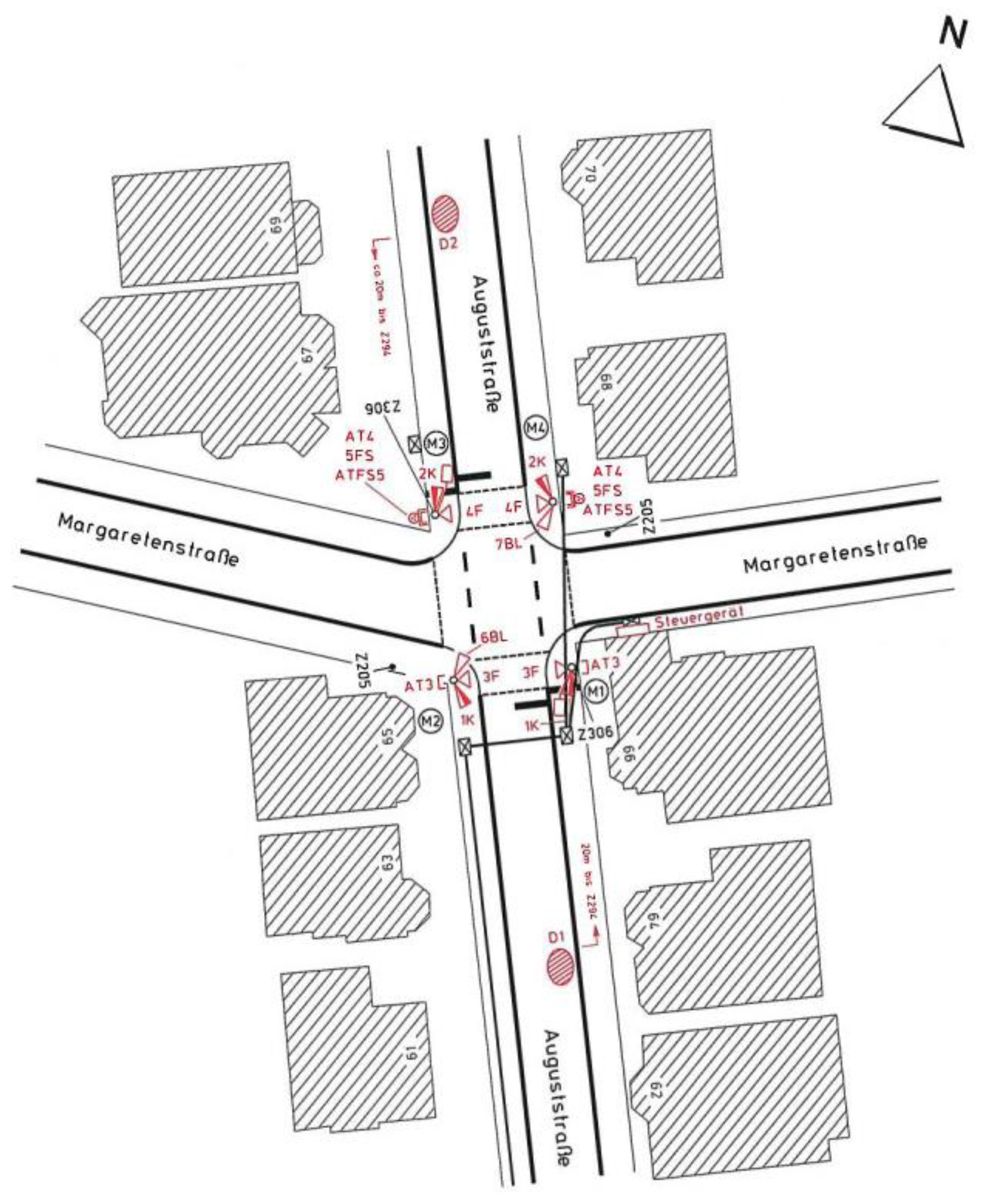
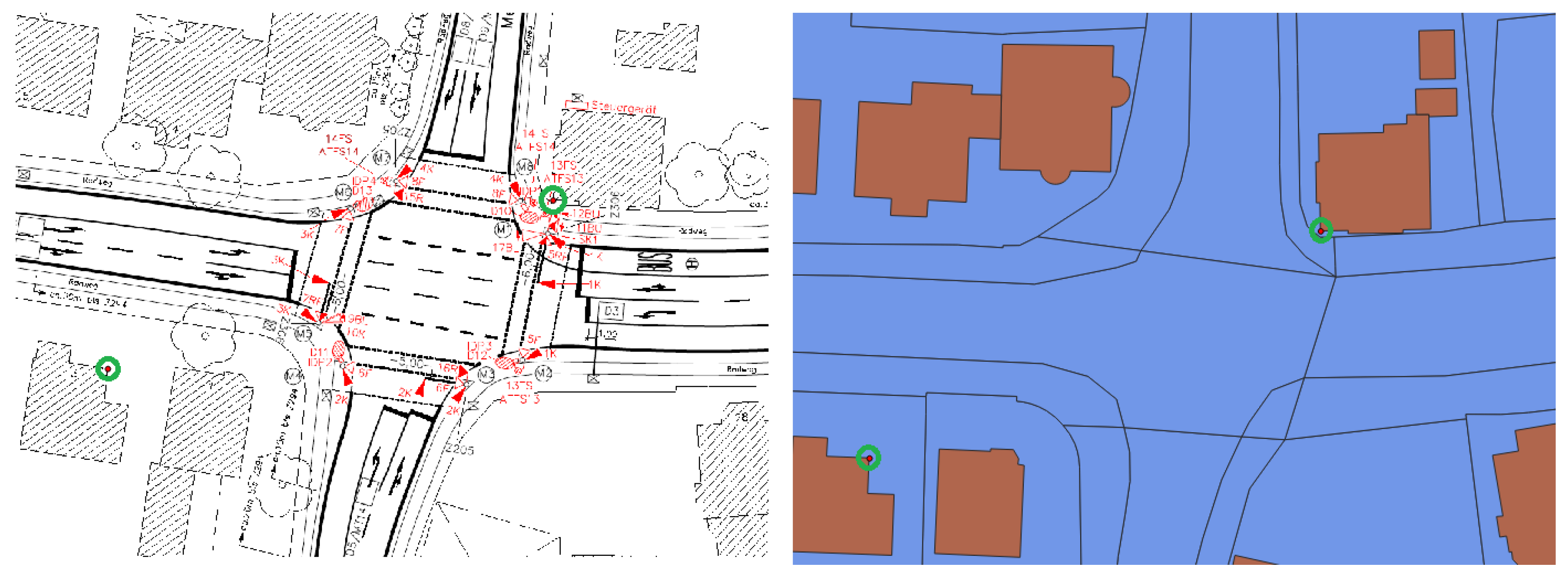
This chapter further describes the data source utilized in this study. The PDF-based site maps depict intersections within the city of Oldenburg in Lower Saxony, Germany. Approximately 153 files featuring intersections with traffic measurements were accessed. These site maps contain digital annotations outlining buildings, roads and traffic measurement locations. The measurement locations are dispersed across various spots within the intersections. In the exemplary map (see Figure 1), measurement points D1–D13 are indicated. Additional markings and shapes serve as internal notations, indicating whether a measurement location corresponds to thermal imaging cameras, radar detection, etc. The arrow positioned at the upper right denotes the northern direction.

Figure 1.
Exemplary map of an intersection with traffic measurement locations in Oldenburg, Germany.
However, several challenges are associated with the PDF files. In some instances, location information is not available as text. Moreover, if the site map is older than 20 years, the legend may lack textual elements. The site map only comprises images in this case. Consequently, all text present on the map is rendered as an image. The site maps that include measurement points are presented solely as images. There is not any technical relationship between the naming conventions of the measurement points and the points themselves. The names can only be visually discerned on the map.
4. Potential Approaches for Geo-Referencing
Geo-referencing can be divided into three central aspects. Rotation represents the turning to a certain degree. Translation allows it to move the origin of the coordinate. Scaling defines the degree of the scale. In this specific use case, a similarity transformation will be applied to change a rectangular into another rectangular coordinate system [21]. This procedure can be applied if there is no bias.
Geo-coordinates of a shape file of the city of Oldenburg that was supplied by the municipal department of geo information and statistics were used. The shape file contains geometric information and coordinates of the buildings and roads with geo-coordinates in the city of Oldenburg. The shape file can be opened via geo information software. The size and position of buildings and roads that are very important for the orientation and the accurate positioning of reference points were calculated by the land surveying office. It can be assumed that the values of the shape file are very accurate as it was gathered by official authorities. As an alternative, OpenStreetMap OSM data could be applied. A huge advantage is that data are for free and openly available. Nonetheless, OSM is based on contributions of the general public. Therefore, the data quality is uncertain. Because everyone who is interested may participate, some inconsistencies may be expected [22]. It can be assumed that the data provided by municipal or government agencies are more reliable regarding the positions of roads and buildings. The corners of the buildings will be used as reference points in the following procedures.
In this specific use case, three potential approaches that are suitable to solve the described problem will be described and compared in the following sub-chapters.
4.1. Geo-Referencing with One Reference Point
The first approach to achieve geo-referencing and similarity transformation involves placing one reference point within the site map. This point is crucial for determining geo-coordinates and ensuring location accuracy. With one reference point, surrounding geolocations can be calculated based on the angle and distance to surrounding points [23]. A single reference point is represented on the map as a pixel and a corresponding geo-coordinate. The reference is typically provided as a commentary within the PDF file. The extraction of its position and content is necessary.
The scale of the map is applied to calculate distances within the map, while rotation can be determined by an arrow indicating the northern direction. Based on the reference point, rotation and scale, coordinate calculations can be performed. However, further examination of available site maps revealed inconsistencies in the accuracy of the arrow that directs to the northern direction. It seems to be that it is often manually placed on the map without proper calibration, leading to inaccuracies in coordinate calculations. The accurate arrow direction is essential for precise results, rendering this method inapplicable if the northern arrow is inaccurate.
4.2. Geo-Referencing with Two Reference Points
Another potential approach involves applying two reference points to calculate rotation and scaling. This method is very similar compared to the geo-referencing process with one reference point, with the addition of an extra reference point included as a PDF commentary to serve as a control point for calculating measurement locations.
To calculate the rotation of the site map, the angular difference between the geo-coordinates and pixel coordinates of both reference points is determined. This difference yields the rotation angle necessary to orient the site map in a northern direction. The atan2 function can be applied to calculate this angle [24]:
Subsequently, the geographic angle between both reference points can be deter-mined based on their respective geographic coordinates. In Formula (2), λ and δ denote the latitude and longitude of the reference points in radians.
The rotation is determined by calculating the difference between the two angles as described in Equation (3). The resulting value represents the degree of rotation required to orient the site map towards the north.
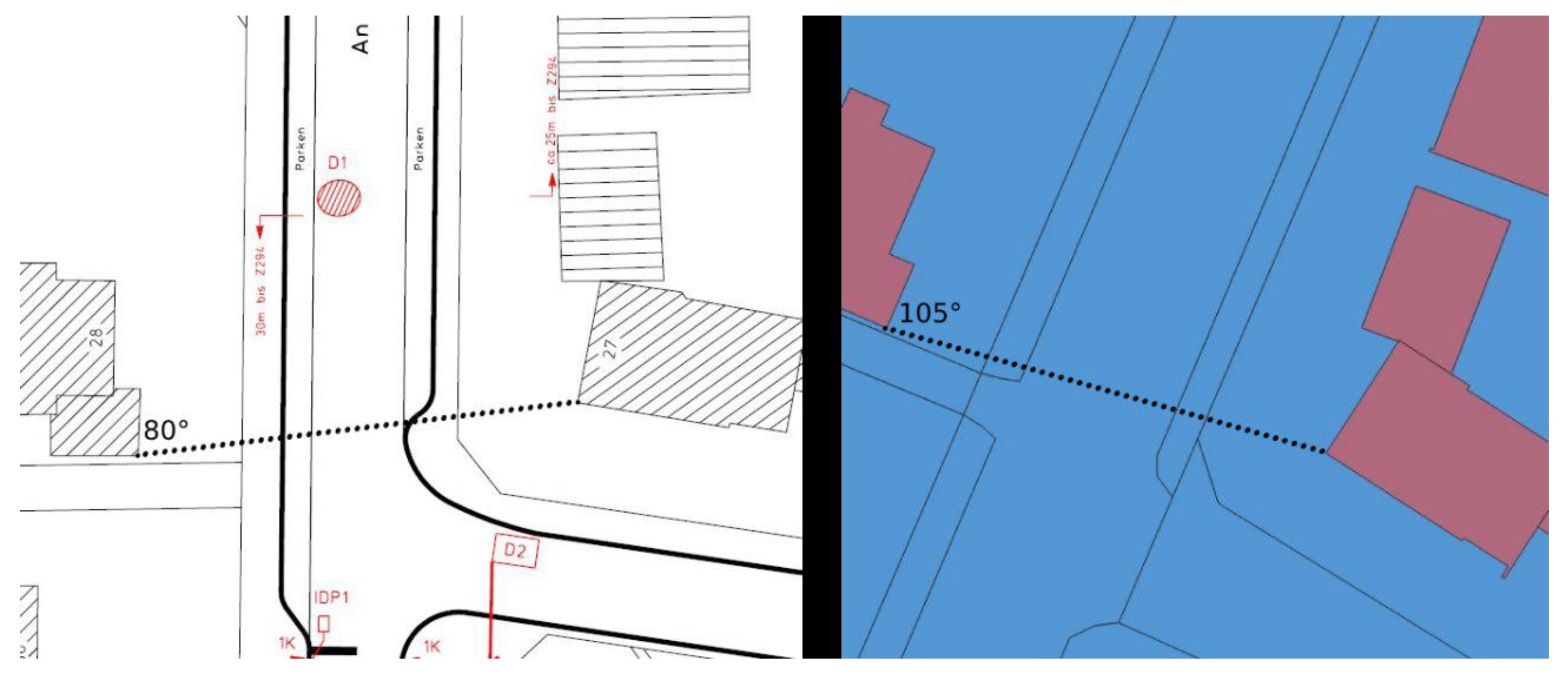
For example, if the angle between two reference points on the site map is 80 degrees, and on the geographical map it is 105 degrees, the site map needs to be rotated by 25 degrees to achieve a northern orientation. The described example is displayed in Figure 2.
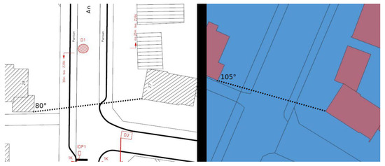
Figure 2.
Different angles of two reference points on the site map (left) and the geographic shape file (right).
To determine the scaling of the site map, the scale factor must be identified. Initially, the distance between the pixel coordinates of the reference points needs to be computed. The Euclidean distance serves as a suitable method for calculating the distance between two points in a two-dimensional coordinate system [25]. The pixel coordinates of the first (x1, y1) and second reference point (x2, y2) are provided in Formula (4):
To compute the geographic distance between the two reference points, the Haversine formula can be utilized [26]. In Equation (5), λ and δ denote the latitude and longitude of the reference points. The symbol R represents the radius of the Earth (6378 km) [27].
The relationship between the geographic distance and the distance on the site map yields the scale. This pixel distance is then transformed into centimeters, considering the pixels per inch (PPI) [28]. Subsequently, the distance is recalculated in meters, and the geographical distance is divided by the pixel distance in meters to obtain the scale of the site map:
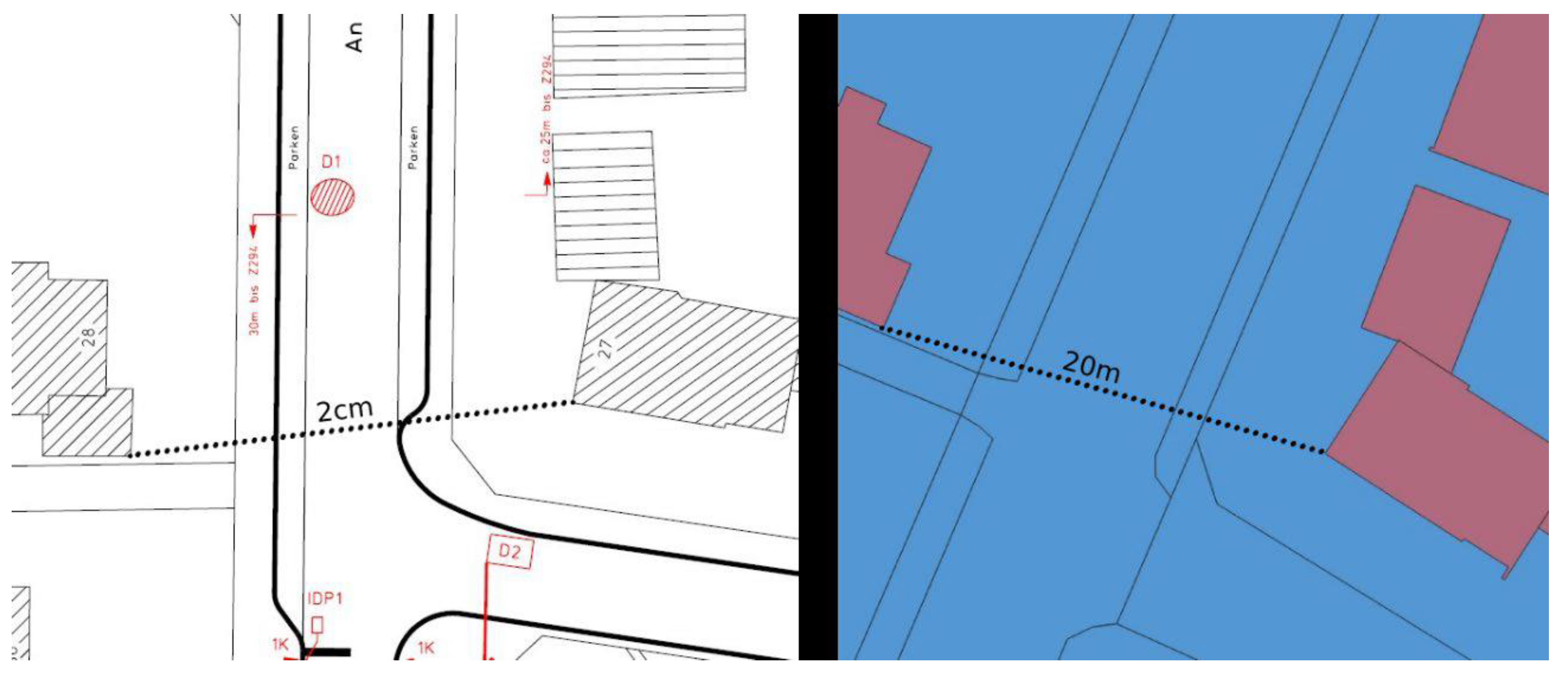
For instance, if the distance between two reference points on the site map is two centimeters and the geographic distance is 20 m, the resulting scale is 1:1000. This example is displayed on the map in Figure 3.
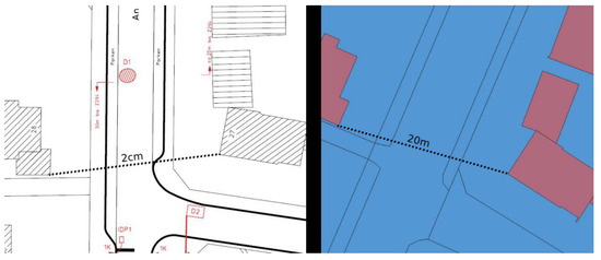
Figure 3.
Distance of two reference points on the site map (left) and in reality (right).
4.3. Geo-Referencing with QGIS
Geo-referencing using the open-source tool QGIS offers another method for extracting geo-references. Spatial data can be aligned with geographical locations [29]. Upon importing the location map into QGIS, the rotation and scaling process can be implemented. This involves setting two Ground Control Points (GCPs) as reference points on the shape file [29]. QGIS displays these control points as red points on the map (as indicated by the green markers in Figure 4).
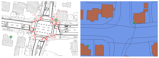
Figure 4.
Exemplary control points at site map (left) and shape file (right).
After setting the control points, the transformation settings must be defined. The Helmert transformation is employed to convert coordinate values into another coordinate reference system, allowing for scaling and rotation based on two control points. This facilitates the transformation to a different coordinate system. The Nearest Neighbor method is utilized as the resampling method to preserve the pixel values unchanged [30]. Before commencing the geo-referencing process, both the geographic and pixel coordinates of the control points are recorded. QGIS generates a Tagged Image File Format file (TIFF, .tif) with the geo-reference. With this step, the geo-referencing process is completed.
The TIFF format, originally developed by Aldus and subsequently extended by Microsoft and Adobe, features a flexible architecture enabling the creation of new information through the definition of new tags [31]. The Geographic Tagged Image File Format (GeoTIFF) is an extension of TIFF designed to store geo-reference information such as details about the reference system or coordinates [32]. Geo-coordinates can be extracted from the GeoTIFF file using the pixel positions (x1, y1) and the coordinates of the measurement locations (t1–t6) according to Formulas (7) and (8) [33].
Lat = t1 + x1 × t2 + y1 × t3
Lon = t4 + x1 × t5 + y1 × t6
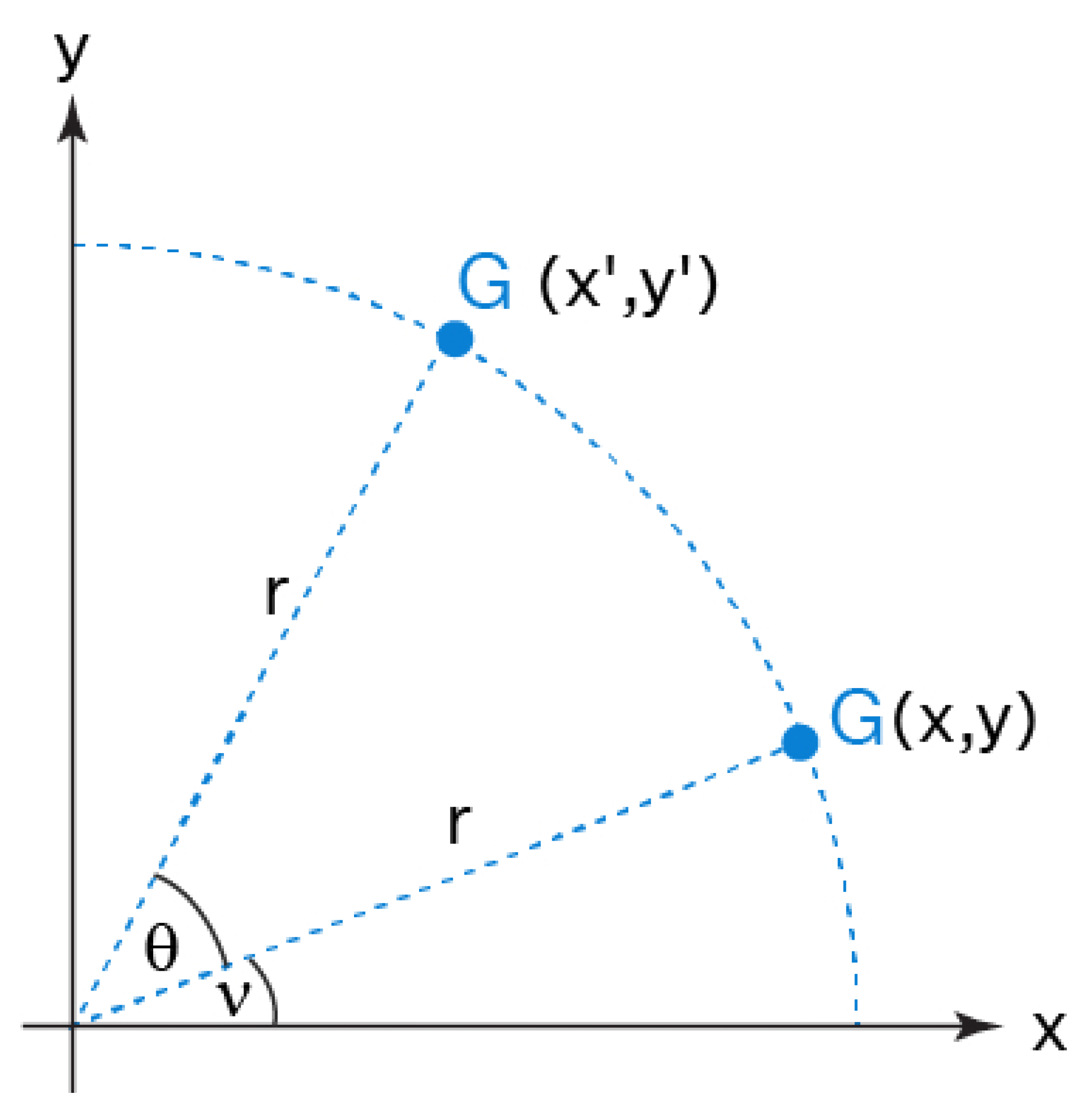
The pixel coordinates of locations in the PDF file need to be adjusted relative to the rotation of the location map in the GeoTIFF file as the site map in the geo-referenced GeoTIFF file is oriented towards the northern direction. A rotation matrix, also known as turning matrix, can be employed to obtain the pixel coordinates. By rotating to a specified degree, the new coordinates (x′, y′) may be determined within the original coordinate system (x, y) [34]. Figure 5 illustrates the visual rotation to the new point in the coordinate system.
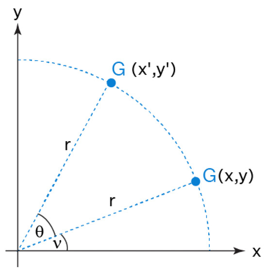
Figure 5.
Visual rotation of a point in a coordinate system from (x, y) to (x′, y′) [34].
In the subsequent rotation matrix Formula (9), α represents the degree of rotation.
The new coordinates are calculated relative to the rotation point, which is the center point of the location map in the GeoTIFF file. The map rotates around this center point, which is located at (0, 0). Therefore, (x, y) must be calculated with respect to this rotation point. The difference between the center point and the coordinate is computed. To obtain the pixel coordinates on the rotated map (x′, y′), the calculated coordinates are added to the center point. Since the size of the new site map has changed due to rotation, the addition is applied with the center point of the image. The center point can be determined by dividing the height and width by 2. In the adjusted Formula (10), (x1, y1) represent the center of the original image, while (x2, y2) denote the center of the rotated location map in the GeoTIFF file [35]. (x′, y′) denote the coordinates in the rotated GeoTIFF file that have been calculated. These can be utilized to extract the geo-coordinates from the GeoTIFF file.
Although various methods are available to obtain the geo-coordinates, utilizing the QGIS tool offers numerous advantages. The method is highly time-efficient because the reference points can be set with a single click on both the site map and the shape file. The pixel coordinates of the site map are then linked with the geo-coordinates from the shape file in a Ground Control Point (GPC) table. QGIS also provides a user-friendly interface. The geo-referencing process may be started with a simple click on the pixel coordinates of the site map and the corresponding geo-coordinate in the shape file. Furthermore, errors can be easily identified and rectified after the geo-referencing process, as QGIS transparently visualizes the site maps alongside the shape file. This enables easy verification of features such as buildings or road alignments. Moreover, the approach is scalable, which allows the geo-referencing of new site maps if a suitable shape file is available. The resulting GeoTIFF file can be utilized for locating traffic measurement locations or other purposes.
5. Assessment and Selection of Geo-Referencing Methods
This chapter aims to compare the presented approaches for geo-referencing in the context of PDF-based site maps to identify the most appropriate solution. The method that relies on one reference point is excluded from this evaluation due to the unreliable alignment of the arrow indicating the Northern direction (see Section 4.1). Therefore, the geo-referencing methods (1) based on two reference points and (2) the QGIS tool are considered. These methods are evaluated based on the time dimension, usability, extensibility, error treatment and accuracy of results.
The time dimension is a crucial aspect for assessing applicability. If the extraction of geo-coordinates is time-consuming, it can lead to increased workload and costs. The assessment is based on a test scenario with ten exemplary site maps. The approach using two reference points took 21 min and 45 s, with an average of two minutes and ten seconds per site map. This method involves manually copying geo-coordinates from the municipality’s shape file and placing them in the site map’s commentary. Conversely, the QGIS solution proved to be more time-efficient. It only required nine minutes and 24 s (approximately 56 s per site map). The primary advantage of the software tool is its streamlined process, where a single click suffices to place reference points on both the site map and the shape file. The pixel coordinates of the site map and the geo-coordinates from the shape file are automatically linked in a Ground Control Point (GCP) table.
Usability is another critical aspect to consider. A method that is easy to apply and understand minimizes the risk of incorrect usage. The availability of a user interface is advantageous in this regard. With the approach using two reference points on the one hand, the manual placement of geo-coordinates into the site map is required. However, there is no user interface to provide feedback on whether the geo-referencing process was applied correctly. Therefore, the correctness of the calculated geo-coordinates must be verified manually. On the other hand, QGIS offers a user-friendly interface. As mentioned previously, the geo-referencing process in QGIS begins with a simple click on the pixel coordinate of the site map and the corresponding geo-coordinate in the shape file. Errors can be detected and corrected after the geo-referencing process as QGIS allows the site map to be displayed transparently in front of the shape file.
Extensibility is a crucial aspect to consider in the decision-making process. If the city administration equips new intersections with measurement technology, the number of site maps may increase. A certain degree of flexibility is needed. In the geo-referencing process with two reference points, new geo-coordinates must be manually placed in the commentary field of the PDF-based site map. As soon as this step is completed, the reference points can be used for geo-referencing new site maps to calculate coordinates for the localization of measurement points. The QGIS method allows the integration of new site maps if a suitable shape file from the municipality or another local authority is available. The resulting GeoTIFF file can then be utilized for the localization of measurement locations. Both methods demonstrate suitability for potential extensions.
After completing the geo-referencing process, it becomes necessary to verify the correctness of the results. Potential corrections of inaccuracies or errors must be feasible, and the monitoring process should be efficient and timesaving. With the two-reference-point approach, manual inspection of the reference coordinates is required. Conversely, the QGIS interface allows the efficient detection of errors, as the site map can be visualized transparently in front of the shape file. This enables easy verification of the position of buildings or roads.
In assessing the accuracy of the geo-referencing processes, the resulting coordinates from the available approaches need to be evaluated. If the same reference points are utilized, it can be expected that, given identical accuracy, the geo-coordinates should correspond to the same location. The accuracy of the extracted coordinates was tested using one site map. The results are displayed in Table 1.

Table 1.
Coordinate deviations of the two reference points and QGIS approaches for geolocation.
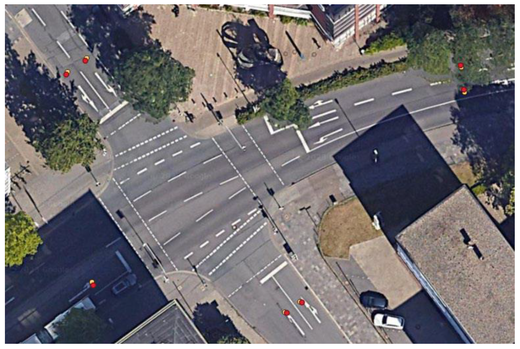
The average deviation of the latitude is approximately 35 cm, while the deviation of the longitude is around 22 cm. Notably, the resulting coordinates accurately align with the correct lane of the road. In Figure 6, the yellow points represent the approach based on two reference points. The red points indicate the results obtained using the QGIS method.

Figure 6.
Extracted geo-coordinates of the two-reference-point (yellow) and QGIS methods (red).
It can be concluded that both methods exhibit similar extraction quality and extensibility. However, the extraction of geo-coordinates from site maps can be achieved more efficiently with the QGIS solution. The QGIS interface enhances improved usability for the user and checking the correctness of results is less time-consuming. Therefore, the QGIS approach should be prioritized in the selection process for further implementation.
6. Limitations, Conclusions and Outlook
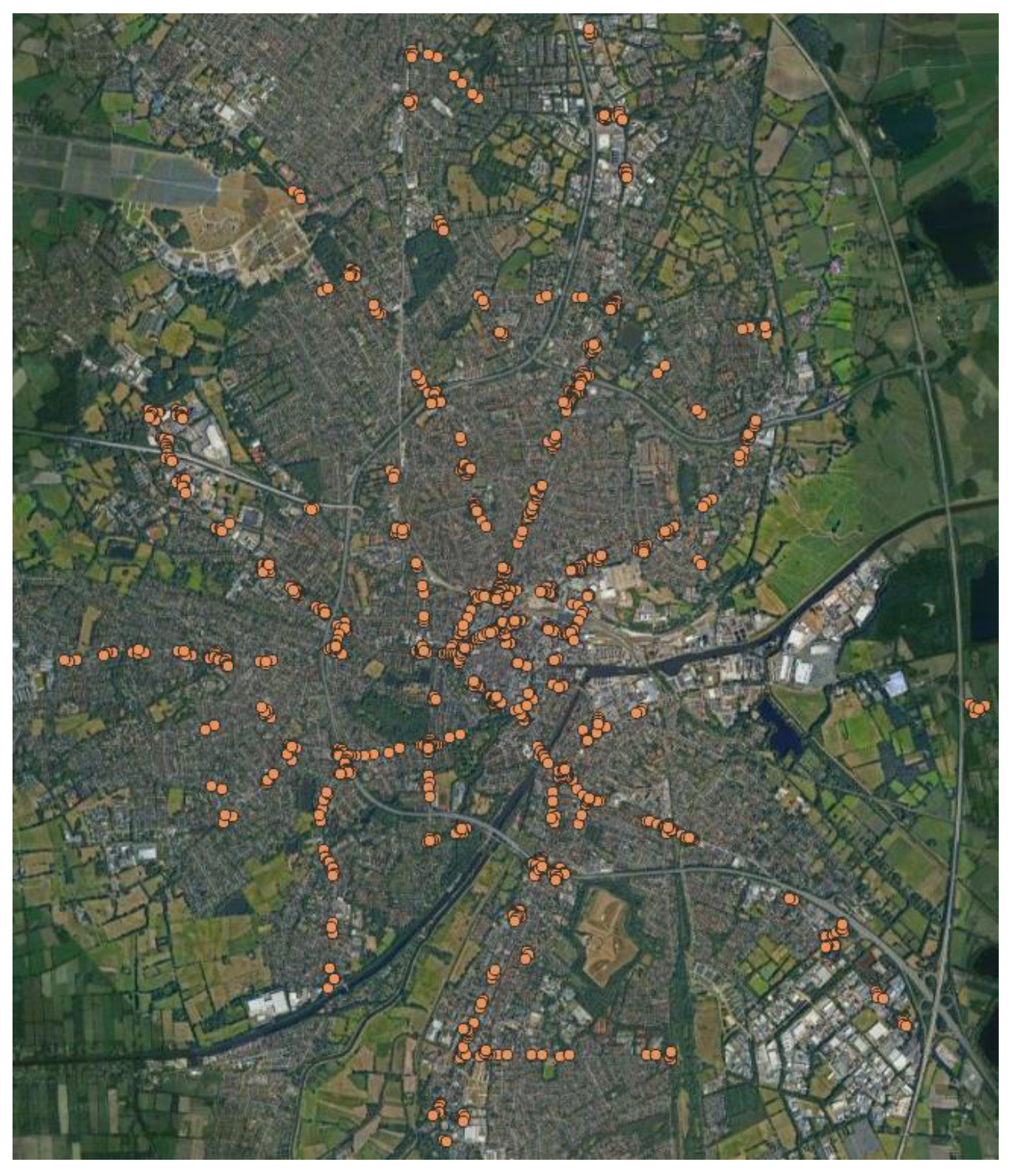
Reliable traffic volume is required not only for the (re-)construction of roads but also to strengthen options of sustainable mobility. Traffic volume data are applied in the decision process to define what is the most suitable alignment of a bike path or the assessment of cycling safety. As delineated, the isolation of geo-coordinates from traffic measurements complicates the utilization of traffic volume for subsequent data-analysis purposes. The absence of stored locations of traffic counters in any database necessitates their extraction from PDF-based site maps. These lack numerical coordinate formats. Thus, the primary aim of this work is to find a suitable and efficient approach to extract the coordinates from the PDF-based site maps. It is crucial to combine traffic volume and locations for stakeholders’ use. For instance, cycling planning experts require traffic volume insights to determine suitable bike path alignments. Geo-coordinates from authoritative shape files should be prioritized compared to OSM data. These may be applied as reference points for the geo-referencing process including translation, rotation and scaling. The successful extraction of geo-coordinates from GeoTIFF files is achieved via QGIS, which is useful with its user-friendly interface and error-handling capabilities. The geo-coordinates are extracted based on the x and y coordinates and can be computed using the rotation matrix formula. A target database structure connecting traffic volume and locations is defined, consisting of two tables linked by a unique station_id. Figure 7 depicts the visualization of over 1400 extracted measurement locations across approximately 150 intersections in the Oldenburg area.
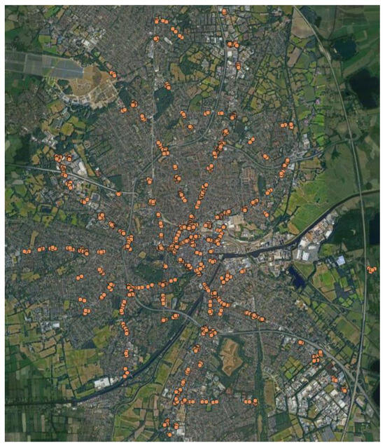
Figure 7.
Visualization of the extracted geolocations in Oldenburg, Germany.
Although the chosen approach is successful in various aspects, there are limitations and areas for potential improvements in future research. Though locations were effectively extracted for different driving lanes, the database lacks information on driving directions for related traffic lanes. Exploring AI methods for automating the extraction process of geo-coordinates could enhance efficiency. Additionally, digital applications linked to the data source, such as the Bike Path Radar (Radweg Radar), offer dynamic, stakeholder-oriented dashboards for cycling planning experts that include key performance indicators related to cycling routes. The established database about traffic volume in Oldenburg is ready for future applications.
In a broader context, the prioritized approach demonstrates significant potential for transferability across various domains. Specifically, within the traffic-planning domain, this methodology can be extended to enhance data accessibility and analysis capabilities. For example, it could be utilized to acquire location data for measurement systems monitoring heavy vehicles, bicycles or pedestrians. By employing similar methodologies, geo-coordinates for such measurement systems could be extracted and integrated into familiar databases.
The selected QGIS solution offers a robust capability to extract geo-coordinates even for objects lacking initial geo-references, presenting a valuable advantage in cases where such coordinates are missing in existing databases. However, successful implementation relies on the presence of reference objects, such as buildings and roads, within the site map. In alternative scenarios, the identification of different objects with geo-coordinates would be necessary.
Another critical requirement is the accessibility to a reliable data source containing the necessary reference objects. In the traffic-related use case that was presented in this contribution, the shape file was provided by the municipal administration. However, in other instances, open-access data sources like OSM may be applied although their reliability is uncertain due to contributions from multiple individuals. Official authorities should be preferred where feasible, ensuring the availability of reliable data sources for research purposes.
Author Contributions
Conceptualization, J.S. and P.S.; methodology, J.S.; software, P.S.; validation, P.S.; formal analysis, J.S.; investigation, P.S.; resources, J.S. and P.S.; data curation, J.S. and P.S.; writing—original draft preparation, J.S.; writing—review and editing, J.S. and P.S.; visualization, P.S.; supervision, J.S., P.S. and J.M.G.; project administration, J.S.; funding acquisition, J.S. All authors have read and agreed to the published version of the manuscript.
Funding
This research was funded by [the Bundesministerium für Digitales und Verkehr (BMDV, German Federal Ministry of Digital and Transport) as part of the mFUND program] grant number [19F2186E] and the APC was funded by [German Federal Ministry of Digital and Transport].
Institutional Review Board Statement
Not applicable.
Informed Consent Statement
Not applicable.
Data Availability Statement
Data are contained within the article.
Acknowledgments
INFRASense is funded by the Bundesministerium für Digitales und Verkehr (BMDV, German Federal Ministry of Digital and Transport) as part of the mFUND program (project number 19F2186E) with a funding amount of around 1.2 Mio. Euro. As part of mFUND the BMDV supports research development projects in the field of databased and digital mobility in-novations. Part of the project funding is the promotion of networking between the stakeholders in politics, business, administration, and research as well as the publication of open data on the Mo-bilithek portal. The data source that was processed in this study was provided by the Department of Traffic and Road Construction, City of Oldenburg, Germany. If there are further queries about the traffic volume data source, please contact Stefan Brandt (stefan.brandt@stadt-oldenburg.de).
Conflicts of Interest
The authors declare no conflict of interest.
References
- Stanley, J.K. Road transport and climate change: Stepping off the greenhouse gas. Transp. Research. Part A Policy Pract. 2011, 45, 1020–1030. [Google Scholar] [CrossRef]
- Hossein Sabbaghian, M.; Llopis-Castelló, D.; García, A. A Safe Infrastructure for Micromobility: The Current State of Knowledge. Sustainability 2023, 15, 10140. [Google Scholar] [CrossRef]
- Gössling, S.; Nicolosi, J.; Litman, T. The Health Cost of Transport in Cities. Curr. Environ. Health Rep. 2021, 8, 196–201. [Google Scholar] [CrossRef] [PubMed]
- Henderson, J.; Gulsrud, M. Street Fights in Copenhagen—Bicycle and Car Politics in a Green Mobility City; Routledge: New York, NY, USA, 2019. [Google Scholar]
- Gössling, S. Urban transport transitions: Copenhagen, City of Cyclists. J. Transp. Geogr. 2023, 33, 196–206. [Google Scholar] [CrossRef]
- DiGioia, J.; Watkins, K.E.; Xu, Y.; Rodgers, M.; Guensler, R. Safety impacts of bicycle infrastructure: A critical review. J. Saf. Res. 2017, 61, 105–119. [Google Scholar] [CrossRef] [PubMed]
- Jaber, A.; Csonka, B. Towards a Sustainable and Safe Future: Mapping Bike Accidents in Urbanized Context. Safety 2023, 9, 60. [Google Scholar] [CrossRef]
- Kapariasa, I.; Liu, P.; Tsakarestos, A.; Edend, N.; Schmitz, P.; Hoadley, S.; Hauptmann, S. Predictive road safety impact assessment of traffic management policies and measures. Case Stud. Transp. Policy 2020, 8, 508–516. [Google Scholar] [CrossRef]
- Guirao, B.; Gálvez-Pérez, D.; Casado-Sanz, N. The impact of the cyclist infrastructure type on bike accidents: The experience of Madrid. Transp. Res. Procedia 2023, 71, 403–410. [Google Scholar] [CrossRef]
- FGSV—Forschungsgesellschaft für Straßen- und Verkehrswesen. Arbeitsgruppe Straßenentwurf Empfehlungen für Radverkehrsanlagen ERA, Ausgabe 2010; FGSV Verlag: Cologne, Germany, 2010; ISBN 978-3-941790-63-6. [Google Scholar]
- Rizwan, P.; Suresh, K.; Babu, M.R. Real-Time Smart Traffic Management System for Smart Cities by Using Internet of Things and Big Data. In Proceedings of the 2016 International Conference on Emerging Technological Trends (ICETT), Kollam, India, 21–22 October 2016; pp. 1–7. [Google Scholar] [CrossRef]
- Wagner, J.M.S.; Scholz, S.; Gennat, M. Verarbeitung, Visualisierung und Kalibrierung von Verkehrsdaten. In Neue Dimensionen der Mobilität—Technische und betriebswirtschaftliche Aspekte; Proff, H., Ed.; Springer Fachmedien: Wiesbaden, Germany, 2020; pp. 477–487. [Google Scholar]
- Verkehrserfassung—Erprobung Von Systemen. Available online: https://www.bast.de/DE/Verkehrstechnik/Fachthemen/v5-verkehrserfassung/verkehrserfassung.html (accessed on 22 February 2024).
- Entwicklung Einer Softwareanwendung zur Qualitätsbestimmung Kommunaler Radverkehrsanlagen auf Basis von Crowdsourcing-Daten—INFRASense. Available online: https://bmdv.bund.de/SharedDocs/DE/Artikel/DG/mfund-projekte/infrasense.html (accessed on 28 February 2024).
- Schering, J.; Säfken, P.; Marx Gómez, J.; Krienke, K.; Gwiasda, P. Data Management of Heterogeneous Bicycle Infrastructure Data. In Proceedings of the EnviroInfo Conference 2023, Munich, Germany, 11–13 October 2023. (in publication process). [Google Scholar]
- FGSV—Forschungsgesellschaft für Straßen- und Verkehrswesen, Arbeitsgruppe Straßenentwurf. H EBRA—Hinweise zur Einheitlichen Bewertung von Radverkehrsanlagen; FGSV Verlag: Cologne, Germany, 2021; ISBN 978-3-86446-296-2. [Google Scholar]
- Pedroso, F.; Angriman, F.; Bellows, A.L.; Taylor, K. Bicycle Use and Cyclist Safety Following Boston’s Bicycle Infrastructure Expansion, 2009–2012. Am. J. Public Health 2016, 106, 2171–2177. [Google Scholar] [CrossRef] [PubMed]
- Buehler, R.; Dill, J. Bikeway Networks: A Review of Effects on Cycling. Transp. Rev. 2016, 36, 9–27. [Google Scholar] [CrossRef]
- Fahrradstadt Oldenburg? Szenarien aus Vergangenheit und Zukunft. Available online: https://www.oldenburg.de/metanavigation/presse/pressemitteilung/news/fahrradstadt-oldenburg-szenarien-aus-vergangenheit-und-zukunft.html (accessed on 29 February 2024).
- De Lange, N. Räumliche Objekte und Bezugssysteme. In Geoinformatik in Theorie und Praxis; Springer Spektrum: Berlin, Germany, 2020; pp. 141–142. [Google Scholar] [CrossRef]
- Kessler, C. OpenStreetMap. In Encyclopedia of GIS, 2nd ed.; Shekhar, S., Xiong, H., Zhou, X., Eds.; Springer: Cham, Switzerland, 2015; pp. 2–4. [Google Scholar] [CrossRef]
- Yao, K.; Du, H.; Ye, Q.; Xu, W. A Power-Efficient Scheme for Outdoor Localization. In Proceedings of the Wireless Algorithms, Systems, and Applications—12th International Conference WASA 2017, Guilin, China, 19–21 June 2017; Ma, L., Khreishah, A., Zhang, Y., Yan, M., Eds.; Springer: Cham, Switzerland, 2017; pp. 534–545. [Google Scholar]
- Kyosev, Y. Topology-Based Modeling of Textile Structures and Their Joint Assemblies: Principles, Algorithms and Limitations; Springer: Cham, Switzerland, 2018. [Google Scholar]
- Jethani, S.; Jain, E.; Thomas, I.S.; Pechetti, H.; Pareek, B.; Gupta, P.; Veeramsetty, V.; Singal, G. Surveillance System for Monitoring Social Distance. In Advanced Computing, 10th International Conference, IACC 2020, Panaji, Goa, India, 5–6 December 2020; Revised Selected Papers, Part I; Garg, D., Wong, K., Sarangapani, J., Gupta, S.K., Eds.; Springer: Singapore, 2021; pp. 100–112. [Google Scholar] [CrossRef]
- Prasetya, D.A.; Nguyen, P.T.; Faizullin, R.; Iswanto, I.; Armay, E.F. Resolving the Shortest Path Problem using the Haversine Algorithm. J. Crit. Rev. 2020, 7, 62–64. [Google Scholar]
- Backhaus, U. Die Größe der Erde und die Entfernung des Mondes: Ein Projekt im Rahmen des Internationalen Jahres der Astronomie 2009 (IYA2009). In Astronomische Phänomene—Beobachtung, Interpretation und Messung; Springer: Berlin, Germany, 2022; pp. 89–111. [Google Scholar]
- Khan, T.; Johanan, J.; Zea, R. Web Developer’s Reference Guide; Packt Publishing: Birmingham, UK, 2016. [Google Scholar]
- Islam, S.; Miles, S.; Menke, K. Mastering Geospatial Development with QGIS 3.x: An In-Depth Guide to Becoming Proficient in Spatial Data Analysis Using QGIS 3.4 and 3.6 with Python, 3rd ed.; Packt Publishing: Birmingham, UK, 2019. [Google Scholar]
- Menke, K.; Pirelli, L.; Smith, R., Jr.; Van Hoesen, J. Mastering QGIS.; Packt Publishing: Birmingham, UK, 2016. [Google Scholar]
- Burger, W.; Burge, M.J. Digital Images. In Digital Image Processing: An Algorithmic Introduction, 3rd ed.; Texts in Computer Science; Springer: Cham, Switzerland, 2022; pp. 14–15. [Google Scholar] [CrossRef]
- Jordan, D.S. Applied Geospatial Data Science with Python: Leverage Geospatial Data Analysis and Modeling to Find Unique Solutions to Environmental Problems; Packt Publishing: Birmingham, UK, 2023. [Google Scholar]
- Warmerdam, F. The Geospatial Data Abstraction Library. In Open Source Approaches in Spatial Data Handling; Hall, B., Leahy, M.G., Eds.; Springer: Berlin, Germany, 2008; pp. 87–104. [Google Scholar]
- Lang, C.B.; Pucker, N. Vektoren und Matrizen. In Mathematische Methoden in der Physik; Springer Spektrum: Berlin, Germany, 2016; pp. 87–153. [Google Scholar] [CrossRef]
- Elias, R. Transformations in 2D Space. In Digital Media; Springer: Cham, Switzerland, 2014; pp. 65–112. [Google Scholar] [CrossRef]
- Birke, M.; Dyck, F.; Kamashidze, M.; Kuhlmann, M.; Schott, M.; Schulte, R.; Tesch, A.; Schering, J.; Säfken, P.; Marx Gómez, J.; et al. Bike Path Radar: New data driven opportunities for bicycle infrastructure planning and improved citizen engagement. In Book of Abstracts of the 7th Annual Meeting of the Cycling Research Board Conference, Wuppertal, Germany, 25–27 October 2023; Bergische Universität Wuppertal: Wuppertal, Germany, 2023; pp. 194–197. Available online: https://radverkehr.uni-wuppertal.de/fileadmin/bauing/radverkehr/Events/CRBAM23/CRBAM23_BookOfAbstracts.pdf (accessed on 29 February 2024).
Disclaimer/Publisher’s Note: The statements, opinions and data contained in all publications are solely those of the individual author(s) and contributor(s) and not of MDPI and/or the editor(s). MDPI and/or the editor(s) disclaim responsibility for any injury to people or property resulting from any ideas, methods, instructions or products referred to in the content. |
© 2024 by the authors. Licensee MDPI, Basel, Switzerland. This article is an open access article distributed under the terms and conditions of the Creative Commons Attribution (CC BY) license (https://creativecommons.org/licenses/by/4.0/).