Abstract
Rock strength is an essential parameter in the design of any underground excavation, and it has become even more relevant as the focus increasingly shifts to sustainable excavations. The heterogeneous nature of rock material makes characterising the strength of rocks a difficult and challenging task. The research results presented in this article compare the impact on the strength when the classic stress paths in laboratory experiments are applied versus when in situ stress paths would be applied. In most laboratory experiments, the rock specimens are free of stress at the beginning of the tests, and the load is increased systematically until failure occurs. Opposite paths occur around an underground excavation; that is, the rock is in equilibrium under a triaxial stress state and at least one stress component decreases while another component may increase. Based on discrete element simulations, the research shows that different stress paths result in different failure envelopes. The impact of this finding is evaluated in the application of wellbore stability (e.g., the minimum or maximum mud weight), whereby it is concluded that failure envelopes, based on stress paths closer to the in situ stress paths, result in a more accurate design. Although the most critical location along the circumference is not different, the required density of the mud is significantly different if the rock strength criteria are based on the more realistic in situ stress paths. This means that a change in the way the strength of rocks is characterised improves the sustainable design of all underground excavations.
1. Introduction
Due to the specific nature of rock material, the characterisation of its strength is a difficult and challenging task. Even so, the strength of rocks is an essential parameter in the design of any underground excavation, and it has become even more relevant as the focus shifts increasingly to sustainable excavations. Among other things, this means that failure or poor design must be eliminated at all costs. This applies to all excavations, including those aimed at creating a sustainable infrastructure for underground storage, transport, and clean energy. However, it also applies to the more traditional mine excavations as well as gas and oil wells. For example, the environmental consequences of the failure of rocks around a gas or oil well are extremely serious, and they can have long-term disastrous consequences.
The strength of rocks is a non-intrinsic parameter of the material. Apart from the characteristics of the material, e.g., its composition, heterogeneities, flaws, and pore distribution, the strength of a rock specimen is influenced by numerous other parameters, i.e., the geometry of the specimens (e.g., their volumes, shapes, and orientations), environmental conditions (e.g., humidity and temperature), the loading rate (e.g., conventional loading rates, dynamic loading, and creep), and the test set-up. The consequence of this is that one should always know all the conditions of the tests that are conducted when determining the strength of rocks. This is the reason tests should be conducted following the suggested methods by the International Society of Rock Mechanics (e.g., [1]) or standard methods by various institutes (e.g., [2,3]) that describe the test conditions. When these recommendations are not followed, this should be clearly stated, including the motivation for the deviation. In this paper, the question is raised concerning whether the stress paths presented in the suggested or standard methods are the most appropriate to quantify rock strength and therefore should be used in the design of in situ excavations.
A recent paper [4] presented the results of a study of the relevance of different stress paths concerning the rock strength and the corresponding failure envelopes. In the paper, it was shown that different stress paths had significant impacts on the strengths that were observed. This means that this parameter also is one of the many parameters that make strength a non-intrinsic parameter. In [4], an overview is given of the research results for stress paths that are different from the ones applied in basic laboratory experiments, i.e., following the suggested methods and standards. In most of these cases, multiple loading–unloading cycles are studied (e.g., [5,6,7]), but the effect on the entire failure envelope is not quantified. In a recent published paper [8], a set of laboratory experiments on diorite specimens was presented with loading and unloading stress paths. These paths were similar to the ones studied using numerical simulations in [4], but they were not identical. (Further, the results of their experiments are discussed in more detail, and they are compared to the results of the simulations in this article).
In most laboratory experiments, specimens are free of stress before the tests start, and the load is increased systematically until failure occurs. Around an underground excavation, e.g., a tunnel or borehole, the opposite path occurs. Before the excavation, the rock is in equilibrium under a triaxial stress state. Following the excavation, at least one stress component decreases, and another component may increase. As a result, the stress paths in classic laboratory experiments are different from the in situ stress paths. The impact of various stress paths on the failure envelopes was studied in [4]. A distinct element model was applied, allowing the simulation of the micro-fracturing of the rock. A small representative volume element (RVE) was considered, and three basic types of stress paths were applied to this RVE, i.e., (1) the conventional loading, (2) the unloading of the minor principal stress, and (3) the simultaneous loading and unloading of the major and minor principal stresses, respectively. The latter stress path is what occurs around a borehole. (See further for a more detailed discussion). The applied loading and unloading rates in the simulations are considered to be similar as in classic laboratory experiments and conventional excavations. So, no dynamic loading or unloading is studied, as observed, for example, during rock bursts or hydraulic fracturing. Very slow stress variations, as occurring during geological processes, are also not part of the study. The details of the two-dimensional RVE are provided in [4], including a schematic diagram of the RVE. The choice of the characteristics of the model was based on the calibrations of our own laboratory experiments [9,10]. The merits of the RVE model were established by simulating published laboratory experiments that were undergoing a complex stress path from another research group [11].
The aim of the current research is to analyse the practical consequences of the earlier findings and to determine whether there is reason to change the engineering practice. The application of these three different stress paths showed a clear effect. The main reason for this is that the micro-fracturing that occurs when loading a rock (from zero or a low stress state) until failure is different from the micro-fracturing that occurs when unloading rocks (from the in situ stress state) till failure. Thus, the failure envelopes are different because of this difference in the weakening processes, i.e., the conventional loading results in the largest strength and uniaxial unloading results in the smallest strength.
The paper focuses on the need to apply more realistic stress paths in the rock characterisation process when studying wellbore stability and, in fact, when designing any excavation where there is a risk of rock fracturing. First, the effect of the three basic stress paths on the failure criteria are presented and discussed, including a more detailed presentation of the RVE model. Second, the wellbore stability for an initial isotropic stress state is discussed, and the effect of considering a stress path closer to the in situ stress path on the design parameters, i.e., the estimation of the maximum and minimum drilling mud pressure. Third, an initial anisotropic stress state is considered and implemented in the design of the borehole.
2. Effect of the Three Basic Stress Paths on Failure Envelopes and Micro-Fracturing Process
Three different loading paths are investigated. All three start from an isotropic stress state, including a zero-stress state. The first type is characterised by an increase in the successive steps of the major principal stress until failure (for a constant minor principal stress). This type of stress path is abbreviated as S1(loa),S3(=). For the second type, the minor principal stress is decreased and the major principal stress remains constant, i.e., S1(=),S3(unl). For the third type, the major principal stress is increased, and the minor principal stress is decreased with the same stress increments, i.e., S1(loa),S3(unl). In comparison to the previous two types, the change in deviatoric stress is larger for the third type.
The set-up of the research project is to repeat a large number of simulations, starting from the same model, i.e., a relatively small RVE. This is impossible to apply in real laboratory conditions since each specimen is different, at least slightly. The focus of the research is on one single parameter, i.e., the impact of different stress paths on the strength. The RVE model should be considered to represent a black box rock. Before applying a stress path, one does not know the strength of the RVE model for a specific stress path. The various input parameters for the RVE model are based on past simulations, whereby the calibration was conducted based on both the observed fracture patterns and measured stress–strain curves [9,10]. Crucial for a correct modelling of the behaviour of rock specimens is that the initiation and growth of fractures are possible in the model. Therefore, the two-dimensional Universal Distinct Element Code (UDEC) is used [12]. The original main application of this code was the simulation of rock blocks and their deformation and relative movements, and that is still the case. However, an intact rock can be approximated by an assembly of individual blocks, whereby these blocks initially are glued together along all contact lines. These contact lines are possible future fracture paths. A contact line (i.e., between two adjacent blocks) does not represent a physical crack as long as it is not activated or has passed the pre-defined failure criterion. The sub-division of the model by contact lines has the advantage that future fractures are composed of relatively straight lines. Thus, the contact lines or elements are given strength properties, and hence, they can fail in shear and/or tension, simulating the occurrence of (micro-)fractures. After activation, the contact elements can deform, slide, and open. The blocks also can deform, e.g., in a linear elastic way. Both the individual blocks and the contact elements within a single model can have different property values. More details on the set-up of the black box RVE model are given in [4], including a schematic diagram of the RVE, and details on the calibration of the input parameters are available in [9,10].
The black box rock in this study has the same geometry, the same stiffness values, and the same values for the properties of the individual blocks as in [4]. Only the characteristics of the contact strength have been changed. In this study, the contacts are characterised by a Mohr–Coulomb criterium with a cohesion of 14 MPa, a friction angle of 30°, and a tensile strength of 7 MPa. In the previous publication, the cohesion was 20 MPa, and the tensile strength was 10 MPa. These values are for the contacts, and they should not be confused with the macro-behaviour of an entire rock specimen. As mentioned above, the failure envelope is unknown prior to the simulations. The contact lines are orientated in such a way that their orientations are distributed equally over individual classes at 30° intervals. Therefore, at a macro-scale, the black box rock behaves as an isotropic rock. So far, the simulations are limited to 2D, and the RVE is a square. The external stresses are applied directly on the model, without any interaction of platens. The reason for this is that the focus is on the behaviour of the rock and not on the simulations of laboratory experiments. No stress–strain curves are recorded. It is assumed that a specimen has failed when 50% of all contact elements have been activated. This percentage seems to be the most reliable. During the variation in the external stress, it is recorded if a contact element fails in tensile, shear, or mixed mode.
Figure 1 presents the results of these simulations. First, a stress path corresponding to loading the RVE in one direction (S1(loa),S3(=)) is presented, starting from an isotropic stress state, i.e., from 0, 5, 10, and 15 MPa (Figure 1: vertical stress paths). The failure load is determined for each simulation. Figure 1 presents the failure envelope in a major vs. minor principal stress diagram. The failure envelope of the uniaxial loading is the one that corresponds the closest to the classic failure envelope of the laboratory experiments. However, there are differences, e.g., there are no platens in the model, and stress is applied instead of displacements. The second set of simulations starts from an isotropic stress state, which is equal to the failed stress (i.e., the major principal stress) simulated in the first set of simulations. In the second set (horizontal stress paths in Figure 1), the minor principal stress is decreased until failure occurs, and the major principal stress remains constant (S1(=),S3(unl)). If there is no effect of the stress path, the failure loads in the second set of simulations should correspond to the confining stresses applied in the first set. The third set of simulations, i.e., S1(loa),S3(unl), also aims to reach the failure loads in the first set of simulations (stress paths under an angle of 45° in Figure 1).

Figure 1.
Failure envelopes for the three basic types of stress paths (i.e., uniaxial loading (S1(loa),S3(=)), uniaxial unloading (S1(=),S3(unl)) and simultaneous loading and unloading (S1(loa),S3(unl))). Start of each stress path (i.e., an isotropic stress state) and failed stress states are indicated by crosses. Each set of three basic types of stress paths is presented by a different colour (four sets in total).
The three failure envelopes are clearly separated (Figure 1). The one that corresponds to the uniaxial loading (S1(loa),S3(=)) results in the strongest strength; e.g., for a zero-confining pressure, the failure load is 55 MPa (Table 1a). The failure envelope of the simultaneous loading and unloading stress paths (S1(loa),S3(unl)) is situated between the uniaxial loading (S1(loa),S3(=)) and uniaxial unloading (S1(=),S3(unl)) envelopes. The strength reduction along the stress path, when comparing the failure load of the uniaxial unloading stress path with the uniaxial loading stress path, is situated between 41% and 43% (Table 1b). A comparison between the simultaneous loading and unloading stress paths and the uniaxial loading shows a strength reduction between 28% and 34% (Table 1c). (Further, these differences are compared to the experimental results published in [8]).

Table 1.
Strength values for the three types of stress paths. (a) Uniaxial loading (S1(loa),S3(=)), i.e., reference for other stress paths; (b) uniaxial unloading (S1(=),S3(unl)) and reduction along stress path in comparison to uniaxial loading; (c) simultaneous loading and unloading (S1(loa),S3(unl)) and reduction along stress path in comparison to uniaxial loading.
When the stress state in a rock changes, micro-fracturing may occur. This is clearly illustrated when acoustic emissions are recorded [7,8,13,14,15,16,17]. The type and amount of micro-fracturing is influenced by the stress level and by the amount of the change in the stress. It is the accumulation of all the micro-fracturing that leads to the ultimate macro-failure of rocks, and this occurs both in laboratory experiments and in situ. The difference between the two applications is that, in most experiments, the test is continued until failure occurs (and sometimes even beyond failure, i.e., further than the maximum stress level), while in situ, the stress redistribution does not necessarily lead to failure. Different micro-fracturing is induced in different stress paths. Hence, micro-fracturing plays an important role when loading or unloading rock specimens. The difference in micro-fracturing results in a difference in the final macro-strength and macro-fracture pattern. The type of contact activation or failure is recorded by the Universal Distinct Element Code (UDEC) [12,18]. There are three modes of contact failure, i.e., in tension, in shear, or in a combination of both. For example, a contact can open (tensile failure), followed, in a later calculation step, by a closure and/or by a shear displacement. The latter two situations are labelled as (1) tensile failure in the past and (2) tensile failure in the past combined with shear failure. The latter is an example of a mixed failure or activation mode. Figure 2 presents the variation in the contact failure modes as a function of the stress path. The three simulations that are directly and indirectly linked to a confining pressure of 15 MPa are presented, i.e., the three stress paths indicated by the light blue colour in Figure 1. In Figure 2, the horizontal axis presents a relative scale between 0% and 100% from the initial load till the failure load. For the first (S1(loa),S3(=)) and third (S1(loa),S3(unl)) types of stress paths, the major principal stress is increased systematically until failure occurs. For the second type (S1(=),S3(unl)), the minor principal stress is decreased systematically until failure occurs. At the top of each graph, the starting and final stresses are indicated as absolute values. (Also, see Table 1). As can be observed, different load intervals are needed to reach 50% of the failed or activated contact elements.
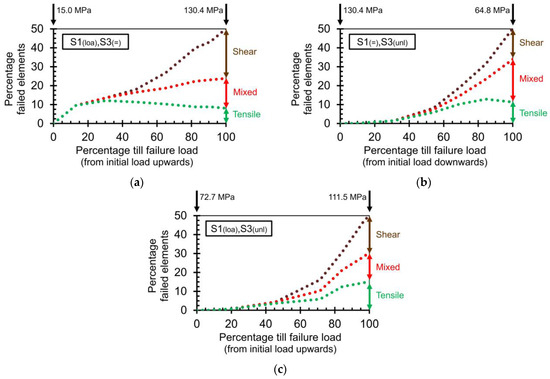
Figure 2.
Variation in the contact failure modes (i.e., tensile-only, shear-only, and mixed modes) as a function of the stress path, i.e., from the initial isotropic stress state till the load level of failure, corresponding to 50% failed contacts. The three types of stress paths are presented for the case, with a confining pressure of 15 MPa during the uniaxial loading (i.e., the three stress paths indicated by the light-blue colour in Figure 1). The initial and final failure loads in absolute values are presented at the top of each graph. (a) Uniaxial loading, S1(loa),S3(=), major principal stress levels are presented; (b) uniaxial unloading, S1(=),S3(unl), minor principal stress levels are presented; (c) simultaneous loading and unloading, S1(loa),S3(unl), major principal stress levels are presented.
For all uniaxial loading simulations, i.e., S1(loa),S3(=), it is typical that the fracturing starts in tension only, and this occurs at an early stage of the increase in the major principal stress (Figure 2a). At around 20% of the failure load (relative to the initial isotropic stress state of 15 MPa), the first contact element also undergoes a shear displacement (mixed mode). At the end of the simulation, i.e., when 50% of all contacts have been activated, about 52% of these activated contacts have failed in shear only and 16% in tension only. The mixed mode represents 32% of the activated contacts. In comparison to the previous stress path, the unloading of the minor principal stress, i.e., S1(=),S3(unl) shows that the first activation of contacts occurs later, i.e., at 20 to 30% of the entire unloading interval (Figure 2b). Again, the first activations are in tension only. When the RVE is assumed to have failed fully, the largest mode of failure type is the mixed mode with about 45% of all activated contacts. The other two modes are 32% for the shear-only mode and 23% for the tension only mode. For the third type of stress path, i.e., S1(loa),S3(unl), characteristics of the stress paths of uniaxial loading and of uniaxial unloading are observed. The first activation takes place at about 20% of the entire stress path, again in the tension-only mode (Figure 2c). At failure, the three modes are relatively similar, i.e., 30%, 32%, and 38% for tension only, mixed mode, and shear only, respectively. All of these observations are similar to the observations for the black box rock RVE, published in [4].
As mentioned above, laboratory experiments on diorite specimens were published recently by Li et al. [8] with loading and unloading stress paths, similar, but not identical, to the ones studied using numerical simulations here and in [4]. A criticism of the numerical simulations of the black box rock RVE could be that it is not supported directly by experimental work. However, the choice of the model characteristics is based on calibrations of our own laboratory experiments [9,10], and the merits of the RVE model were established by simulating published laboratory experiments undergoing a complex stress path from another research group [11]. Also, one should not forget that the whole set-up of the RVE is just to eliminate certain shortcomings of experimental work, e.g., problems linked to repeatability, the effect of size, and the impact of platens. All this does not mean that a comparison with experimental work is not important. The experiments on the diorite specimens [8] consider three stress paths like the three types of stress paths applied above. All experiments are on cylindrical specimens, and the starting point is an isotropic stress state. A first set is the classic triaxial compression loading, whereby the confining stress is kept constant. So, this set follows uniaxial loading simulations, i.e., S1(loa),S3(=). For the two other sets of stress paths, the axial stress is first increased up to 80% of its maximum strength for the corresponding confining stress, i.e., the strength determined in the first set of experiments. For the second set of stress paths, the confining stress is decreased, while the axial stress is kept constant at the 80% level. The third set applies both a loading of the axial stress from the 80% level and an unloading of the confining stress. The unloading rate is twice the loading rate. Even though the starting point of the uniaxial unloading and that of the simultaneous loading and unloading are much closer to the failure envelope of the first set of stress paths, a significant difference is noted between the failure envelope of the classic experiments and the ones of the two other sets. The latter result in a significantly lower strength. The impact between the second and third set is not clear. For example, when analysing the data for the uniaxial unloading, a strength reduction of 42 to 52% is observed when the same calculation is applied as is applied for the RVE results. For the latter, this reduction is situated between 41% and 43% (Table 1b). The larger strength reduction in the published experiments [8] is logical since, during the experiments, the axial load first is increased from the isotropic stress state until it reaches 80% of its strength. During this interval, micro-fractures occur, and the specimen is weakened. This is clearly illustrated in Figure 2a. At the 80% level, about 75% of the activated contacts at failure already have been activated.
3. Effect of the Stress Path on a Wellbore Stability Analysis
The design of a wellbore is very complex, and numerous aspects play significant roles [19,20,21,22,23,24]. The aim of the paper is not to summarize and discuss all of these aspects. The focus is on a single aspect of such a design, i.e., the geo-mechanical determination of the mud weight interval [19,22,23,24], so that no new fractures are induced around the borehole wall. The aim of the paper is to evaluate what the impact would be on the mud weight if the rock strength or the failure envelope were to be determined differently from how it is currently carried out, i.e., by applying stress paths that are closer to the in situ stress paths than the typical stress paths applied in laboratory experiments. Note that the presented results are a first evaluation and are not yet a practical engineering design. Some assumptions are made for this first evaluation. At a later stage, more complex models and approaches could be considered. First, a 2D approach is applied, assuming that the critical plane is perpendicular to the borehole axis. This assumption is realistic if the axial stress is the intermediate principal stress component. If this is not the case, a 3D approach is needed or another 2D section should be considered (e.g., situated along the axial and a radial orientation). Second, it is assumed that all stresses are positive (i.e., compressive stresses at the macro-scale), i.e., only the risk of shear macro-fracturing is integrated in the model (and thus not tensile failure at the macro-scale). Tensile activation may occur at the scale of a contact element, as is illustrated in Figure 2. In situ, tensile failure at the macro-scale may occur around a borehole, but this aspect is not integrated in the current model. Third, it is assumed that the pore pressure is equal to zero. Although for a real and full design, these three assumptions are relevant, they do not prevent the crucial question from being explored, i.e., should one start to characterise the rock strength or the failure envelope differently?
First, an initial isotropic stress state is studied, which results in a relatively easy stress redistribution around a circular opening, i.e., the stress state at all points of the borehole wall is the same. Second, the initial stress state is anisotropic, whereby the axial direction corresponds to the intermediate principal stress component.
3.1. Initial Isotropic Stress State
The evaluation of the redistribution of the stress is relatively easy if the initial state of the stress is isotropic. Before drilling the hole, all directions are principal stress directions, and the circles of Mohr, which represent the stress state, are points. In a major–minor principal stress diagram, the stress state is situated along the 45° line. After drilling the hole and away from the bottom of the hole, the stress redistribution along radial lines (i.e., through the centre of the hole) is the same for all orientations of the radial line, at least if the rock is homogeneous, continuous, and isotropic. The radial and tangential directions are the principal stress directions, and the most critical point is situated on the wall of the borehole. All points along the circumference have the same criticality. Again, this is the case for a rock that is homogeneous, continuous, and isotropic. If, on the other hand, there was a spot along the circumference that is a weak spot, the first fracture would occur at this spot, and the original easy stress redistribution would not necessarily be valid anymore.
As mentioned above, the central question of the research is whether the current practices of determining the rock strength or the failure envelopes are the right procedures or if it would be more appropriate to apply a stress path closer to the in situ stress path. To address this question, some calculations of minimum mud weights are conducted for different values of the initial isotropic stress state.
Three initial stress values are studied, i.e., 25, 50, and 75 MPa. One could assume that these values correspond to an approximate depth of 1, 2, and 3 km, respectively. These three depths cover the range of typical borehole depths well. The pore pressure is assumed to be zero. In the hypothetical case in which there is no well pressure, the stress state along the circumference is in a 2D approach a radial (principal) stress of 0 MPa and a tangential (principal) stress of 50, 100, and 150 MPa, respectively (i.e., two times the initial isotropic stress level). These values are calculated based on the linear elastic theory and the basic formulas [19,22,23,24]. The in situ stress path can be assumed to correspond with the third basic type of stress paths, i.e., the simultaneous loading and unloading with the same increments (the 45° lines in Figure 1). The axial stress remains constant, i.e., the value of the initial isotropic stress.
Based on the results of the black box rock RVE, the conclusion is that for a depth of 1 km, no shear macro-fracture is induced if the strength is determined by a stress path of uniaxial loading. The calculated final tangential stress of 50 MPa (radial stress is equal to zero) is less than the intersection of 55 MPa for the type 1 failure envelope (S1(loa),S3(=); black line in Figure 3, Table 1a). However, the intersection of the failure envelope with the major principal stress axis for the third type of stress path (S1(loa),S3(unl); blue line in Figure 3), i.e., 30 MPa, is less than the calculated tangential stress of 50 MPa. Hence, the rock would fail. For the other two depths, the tangential stress is sufficiently large, so for these two failure envelopes, shear macro-fracturing occurs. Of course, if the depth is 500 m, the tangential stress is only 25 MPa, i.e., lower than both failure envelopes. Only the first and third stress paths are discussed here. The first is discussed because it corresponds to the loading in the classic characterisation. The third is discussed because it corresponds to the stress variation occurring in situ, i.e., the radial stress is decreased, and the tangential stress is increased with the same stress increments.
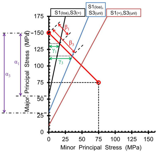
Figure 3.
Failure envelopes for the three basic types of stress paths (see also Figure 1) and illustration of various ways to define the criticality (α, β, γ). Case of an initial isotropic stress state of 75 MPa. Red line corresponds to stress path for a linear elastic calculation.
The variation in the contact failure modes as a function of the stress path for the three cases is similar to the variation presented in Figure 2c. At failure, the three modes of micro-fracturing are distributed nearly equally (i.e., tension only, mixed mode, and shear only). For example, at the moment of failure for the initial isotropic stress state of 75 MPa, the percentages of failed contacts are 28%, 38%, and 34% for the tension-only mode, the mixed mode, and the shear-only mode, respectively. The first activation takes place at about 20% of the entire stress path and is in the tension-only mode.
The conclusion of this first set of calculations is that, for certain stress levels, the chosen stress path for the characterisation of rock strength can make the difference between predicting failure correctly and non-failure incorrectly. The degree of criticality or of safety is different for all stress levels. There are various ways to define this criticality, i.e., the amount above the failure envelopes. The simplest one is just looking at the difference between the tangential stress calculated by the linear elastic theory and the intersection of the failure envelope with the vertical axis (intervals α in Figure 3). For the three depths, these differences for S1(loa),S3(=) are −5 MPa (no failure), 45 MPa, and 95 MPa, respectively (Table 2). For S1(loa),S3(unl), these differences are larger, i.e., 20 MPa, 70 MPa, and 120 MPa, respectively. A second way is to look at the interval between the stress state calculated in the linear elastic domain and the failure envelope along the stress path, i.e., the 45° line (intervals β in Figure 3). These values also can be expressed as a percentage of the total interval of possible stress change, i.e., for a linear elastic calculation (Table 2). The intervals for the stress paths (S1(loa),S3(unl)) are about two to three times larger than the intervals for the stress paths (S1(loa),S3(=)). For example, for an initial isotropic stress state of 50 MPa, the values β1 and β3 are equal to 11.2 MPa and 29.7 MPa, respectively. So, this means that macro-failure occurs about 8.5 MPa earlier when the stress path is equal to the in situ stress path in comparison to the conventional strength characterisation. The third way applied is the most visual and easily interpretable method, i.e., by calculating the minimum wellbore pressure needed to eliminate the risk of a shear macro-fracture being induced. By applying this pressure, the radial stress on the circumference is increased by its value and the tangential stress is decreased by it. This is indicated by the intervals γ in Figure 3 and Table 2. By using the depths indicated above, this minimum wellbore pressure is translated into a minimum mud weight. Looking blindly at the figures, it means that the mud density when characterising a rock by the third type of stress path (S1(loa),S3(unl)) should be two to three times larger than the density when the rock is characterised by the first type of stress path (S1(loa),S3(=)). For example, for the deepest section (i.e., 3000 m), the minimum density is 0.546 kg/dm3 and 1.171 kg/dm3, respectively. From a practical perspective and for this particular black box rock, one must point out that there is no risk of shear macro-failure in four of the six combinations if the density is 1 kg/dm3. For a weaker material, the latter is not necessarily still true. However, the conclusion remains that the impact of rock characterisation by one of the two stress paths is significant.
Table 2.
Stress redistribution for an initial isotropic stress state and parameters describing the criticality of failure at the borehole wall (see Figure 3), including the minimum mud weight.
3.2. Initial Anisotropic Stress State
Even for the relatively simple case of a circular excavation, the stress state in each location along the circumference is different if the initial stress state is anisotropic (Figure 4). As one of the conclusions of the previous study was that failure envelopes are different for each different stress path, it means that the study of a circular excavation becomes very complex. Here, the focus is on the quantification of this complexity. So far, the simulations of an RVE have shown that the various stress paths result in failure envelopes that are situated between the one whereby the major principal stress is increased (type 1, S1(loa),S3(=), or a stress path comparable to the loading in classic laboratory experiments) and the one whereby the minor principal stress is decreased (type 2, S1(=),S3(unl)). Hence, by conducting experiments for these two types of stress paths, one gets a relatively good idea about the possible effect of a stress path on the failure envelope. If the second type of stress path (S1(=),S3(unl)) is applied, but starting from an anisotropic stress state, the failure envelope for a larger anisotropy moves closer to the one of the conventional loading paths. This is studied for the case in which the initial minor principal stress is decreased.
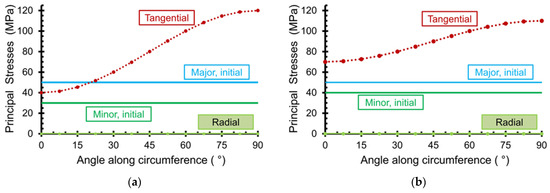
Figure 4.
Stress redistribution along borehole wall for the initial anisotropic stress state. (a) 50 and 30 MPa; (b) 50 and 40 MPa. 0° corresponds to orientation of initial major principal stress (Figure 5).
In comparison to an initial isotropic stress state, the stress redistribution around a borehole for the initial anisotropic stress state is more complex. The tangential stress is different in each point of the circumference (Figure 4) (to be precise, per quarter of the circumference). The two extreme values are reached on the two radial lines that correspond to the orientation of the initial major and minor principal stresses, i.e., for the angles of 0° and 90°, respectively. For these two angles, the orientation of the principal stresses does not change, i.e., it is always in the radial and tangential direction in comparison to the borehole (Figure 5). Along any other radial line, the principal stress orientations before drilling are different from the principal stress orientations on the circumference of the borehole wall. The latter are always radial and tangential. For the radial line that corresponds to the orientation of the minor principal stresses (i.e., 90° in Figure 4 and Figure 5), this orientation (i.e., radial orientation) remains the orientation of the minor principal stress. However, for the radial line that corresponds to the orientation of the major principal stresses (i.e., 0°), this orientation (i.e., the radial orientation) evolves from the major to the minor principal stress orientation. All of these aspects should be considered when analysing the RVE behaviour.

Figure 5.
Conceptual drawing of orientation of principal stresses (each in a different colour) along borehole wall. (a) Before drilling; (b) after drilling.
In earlier studies, we specifically analysed the effect of the principal stress orientations. Although the aim of the research and the experimental set-up were different from the current research, the importance of the change in stress orientation was illustrated clearly. Some experiments focused on cyclic Brazilian tensile tests, whereby the disks were rotated before reaching the final macro-failure [25]. These tests aimed to evaluate the sensitivity of the Kaiser effect towards the principal stress orientation. The experiments and the discrete simulations showed that the effect gradually became less pronounced as the rotation angle increased. In another study, the damage around a circular opening was studied [14] and two configurations were investigated. In the first set of experiments, the damage was induced mainly by shear stresses (only macro-compressive stresses were present). In the second set, the tangential stresses were tensile stresses at the macro-scale. For specimens first damaged by a tensile macro-stress, followed by macro-compressive stresses, more damage was observed than in the other sequence.
3.2.1. No Change in the Orientation of the Principal Stresses
The two points situated at the angles of 0° and 90° along the circumference are discussed first. As illustrated in Figure 5, the radial and tangential orientations are principal stress orientations before and after drilling the borehole. Elastic calculations clearly show that the point at 90° is more critical than the point at 0°, i.e., for shear failure at a macroscopic scale. An unknown factor for all analyses presented in this paper is how the stress state exactly evolves from before drilling the hole until after the hole has been drilled. For all simulations, it is assumed that the stress paths follow linear variations in the major-minor principal stress diagrams. This assumption seems to be realistic, at least if one considers a 2D approach. For a 3D model and taking the stress variation around the bottom of the hole into account, the real stress paths are most likely more complex [21,23,24,26].
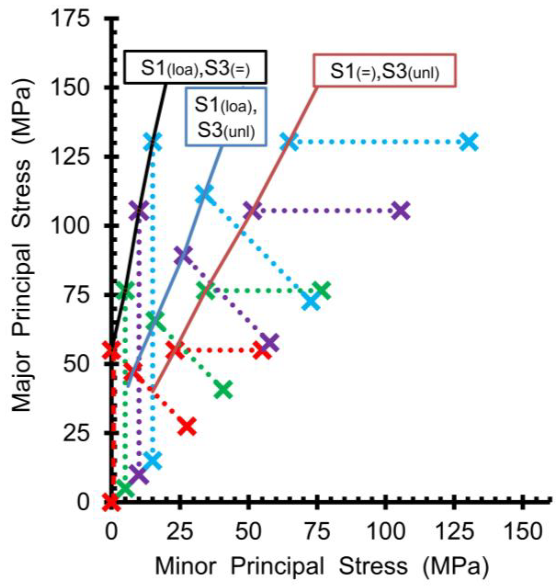
For the point at 90°, the situation is comparable to the results presented earlier. The tangential and radial orientations correspond to the major and minor principal stress orientations over the entire stress path, respectively. Four different initial anisotropic stress states are studied, i.e., (30, 50), (40, 50), (45, 75), and (60, 75) MPa (Figure 6 and Table 3). The same method used above is applied here. For each initial stress state, the final stress state is calculated for the borehole wall, based on a linear elastic calculation. The RVE model is loaded in the vertical direction (i.e., corresponding to the tangential orientation) and unloaded in the horizontal direction (i.e., corresponding to the radial orientation) aiming at the final linear elastic stress state (Figure 6a). However, the latter is, in most cases, never reached because failure occurs somewhere along the stress path. In other words, the maximum strength is calculated for each stress path (Figure 6a; Table 3a). These four strength values correspond to four different failure envelopes, i.e., for each of the four stress paths. The four simulated strength values are situated between the failure envelopes of uniaxial loading (type 1; black line in Figure 6a) and of the simultaneous loading and unloading with the same increments (type 3; blue line). The larger the initial anisotropy, the closer the strength for the in situ stress paths is situated to the failure envelopes of uniaxial loading. Most likely, the behaviour for the various stress paths is a combination of the mentioned basic types of stress paths (black and blue lines). For a larger anisotropy, the in situ stress path is oriented more vertically and thus more towards the type of uniaxial loading (and farther away from the type of stress path under an angle of 45°).
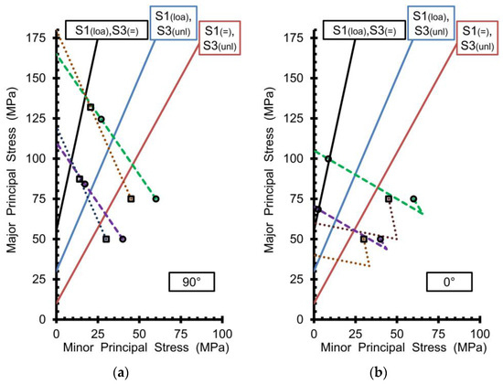
Figure 6.
Stress paths between the initial anisotropic stress state and the linear elastic calculation of the stress state on the borehole wall. The starting points and the stress states at failure are indicated by squares and circles. All information is superimposed on the failure envelopes for the three basic types of stress paths (see Figure 1). Four different anisotropic stress states are studied (each with a different colour), i.e., (30, 50), (40, 50), (45, 75), and (60, 75) MPa. (a) 90° angle (see Figure 5); (b) 0° angle.
Table 3.
Stress redistribution for the initial anisotropic stress state and parameters describing the criticality of failure at the borehole wall (see Figure 3), including the minimum mud weight. (a) For point corresponding to 90° along the circumference; (b) for point corresponding to 0° along the circumference.
It is important to stress again that, in the approach put forward in this study, the strength values in Table 3a are considered to be the “correct” ones (indicated by the label “real”; see also the squares and circles in Figure 6a). In comparison with these values, the values determined by stress path type 1 (S1(loa),S3(=)) are an overestimation of the “real” strength, and the ones for the type 3 stress path (S1(loa),S3(unl)) are an underestimation of the “real” strength. The type 2 stress path ((S1(=),S3(unl), brown line) results in a larger underestimation and is not integrated in Table 3. In Table 3a, the values for the various parameters of criticality are presented for the type 1 stress path, the in situ or real stress path, and the type 3 stress path. For detailed values, the reader is referred to Table 3a, but the conclusion is that the values for the in situ (or real) stress paths are significantly different from the two basic types of stress paths.
This conclusion also is valid for the calculated mud weight (Table 3a). The mud weight only can be calculated if a depth is known. Here, it is assumed that the major principal stress corresponds to the depth. So, the value of 50 MPa corresponds to an approximate depth of 2000 m, and the value of 75 MPa corresponds to 3000 m. So, the lay-out could be a horizontal borehole at these depths or a vertical borehole whereby the major horizontal principal stress is equal to the vertical (axial) stress. For example, for an initial stress state of (60, 75) MPa, the minimum mud weight for the real stress path is 1.009 kg/dm3. When one determines the strength by applying stress paths similar to the conventional testing (type 1), the minimum mud weight is only 0.632 kg/dm3. This is a significant difference, and it cannot be neglected. When comparing the various values of the minimum mud weights (Table 3a), there is a peculiar observation. For both basic types of stress paths, the minimum mud weight is greater when the initial anisotropy is larger (i.e., comparing the first column to the second column and comparing the third column to the fourth column). It is just the opposite for the in situ or real stress paths. The reason for this is that, in the case of the real stress paths, both the linear elastic calculated stress values and the strength values are different as a function of the initial anisotropy. For the cases with an initial major principal stress of 75 MPa, the linear elastic calculated stress values are 180 MPa (third column) and 165 MPa (fourth column) for the large and small initial anisotropy, respectively. As can be seen in Figure 6a, the two real stress paths cross. This means that, the value of 180 MPa is farther away from the basic types of failure envelopes than the value of 165 MPa. So, a larger minimum mud weight is needed. When considering the real stress path, the linear elastic value of 180 MPa is situated closer to the corresponding calculated strength than it is to the value of 165 MPa and its corresponding strength value. Note that the entire four failure envelopes that correspond to the four real or in situ stress paths are not drawn in Figure 6a; only one point of each failure envelope is represented. In conclusion, the calculations of the critical mud weights illustrate well the importance of applying a stress path close to the in situ stress path when testing rocks. The calculations also highlight the complexity of the problem.
As pointed out in Figure 4 above, the point that corresponds to an angle of 90° along the circumference is more critical than the 0° point when studying macroscopic shear fracturing. In Figure 6b and Table 3b, the same exercise is repeated for an angle of 0°. A significant difference between the two points is that for 0°, the orientation of the major and minor principal stresses switches along the stress path (Figure 5). Initially, the radial stress component is the major principal stress. Along the stress path, this component decreases, and at a certain moment, it becomes equal to the tangential stress, which increases systematically starting from the initial minor principal stress (Figure 6b). Afterwards, the tangential stress increases further and the radial stress decreases. Table 3b gives the stress value for which both components are equal. The result of switching between the principal stress orientations is that the global stress state first evolves away from the failure envelopes (Figure 6b). At the moment of this switch, the circle of Mohr is represented by a point. During that part of the entire stress variation, no micro-fracturing is induced (Figure 7b). For the two cases with the largest anisotropy, no failure occurs (Figure 6b). For the other two cases, the strength following the real stress path is similar to the strength that corresponds to the type 1 stress path (S1(loa),S3(=)).
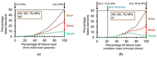
Figure 7.
Variation in the contact failure modes (i.e., tensile-only, shear-only, and mixed modes) as a function of the stress path, i.e., from the initial stress state of (60, 75) MPa till the load level of failure, corresponding to 50% failed contacts. (a) 90° angle (see Figure 5); (b) 0° angle.
In Figure 7, the variation in the three contact failure modes is presented as a function of the full in situ stress path for the case of an initial stress state of (60, 75) MPa and for an angle of 90° and 0°. As mentioned earlier, during the stress relaxation for an angle of 0°, no contacts are activated (Figure 7b). At the moment of failure (i.e., 50% of all contacts have been activated), the main activation mode is shear (55% of all activated contacts in the shear-only mode and 35% in the mixed mode). The activation in the tensile-only mode is small (10% of all activated contacts). The overall shape of the curves for a 0° angle is comparable to the type 1 stress path (Figure 2a and Figure 7b), although the decrease in the tensile-only mode is more pronounced in Figure 7b. Part of the explanation could be that the strength following the real stress path is situated close to the type 1 failure envelope (S1(loa),S3(=)). For an angle of 90° (Figure 7a), the activation in shear only is less dominant than for 0° (Figure 7b). For 90°, the percentages of all activated contacts are 20% tensile-only mode, 37% mixed mode and 43% shear-only mode. The situation at failure is similar to the type 1 stress path (Figure 2a).
3.2.2. Change in the Orientation of the Principal Stresses
Apart from the two points discussed above, the orientation of the principal stresses for the other points is different between the initial stress state and the final stress state along the borehole wall. This means that both the sizes and the orientations of the principal stresses change. For these variations, it is assumed that the size of the principal stresses follows a linear variation in successive steps and that the orientation changes simultaneously. This is illustrated in Figure 8 for the point on the circumference at an angle of 45°. For this angle, the final normal stresses on the planes of 0° and 90° (i.e., the original principal stress orientations) are equal. (See the red triangle for the final (i.e., largest) Mohr circle). Note that only a limited number of successive steps are presented in Figure 8. Along the entire stress path, first, the normal stress increases, and this is followed by a decrease for one of these two planes (illustrated by the right set of triangles). For the other plane, first, there is a decrease in the normal stress, and this is followed by an increase (the left set of triangles). Along the entire stress path, there is a systematic increase in the shear stresses on these planes of 0° and 90°. For the orientations closer to 0° than 45°, the principal stress paths also cross, similar to the case of 0° (Figure 6b).
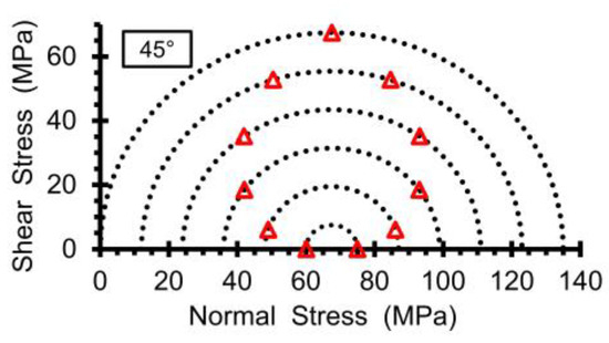
Figure 8.
Evolution of the stress state starting from the initial anisotropic stress of (60, 75) MPa till the stress state of (0, 135) MPa, based on linear elastic calculations. Red triangles represent the combination of normal and shear stresses for the successive Mohr circles, acting on the planes with an orientation of 0° and 90°.
For the initial four principal stress combinations, the strength values following the real stress paths for the point at an angle of 45° along the circumference are situated relatively close to the type 1 failure envelope (S1(loa),S3(=); Figure 9). Note that the point of 45° along the circumference in most cases is situated outside the danger zone for a macroscopic shear fracture [20]. The stress path applied here, i.e., with a systematic change in principal stress orientation, is globally an unknown territory in rock characterisation, and the translation of it in laboratory experiments is far from evident. In the experiments by Lavrov et al. [25], a systematic change in principal stress orientations was applied, but it was for Brazilian tensile tests and for cyclic testing, which is different from the stress variation studied here. The black box RVE simulation indicates that the amount of the tensile-only mode of activation is very limited over the entire stress path (Figure 10). When 50% of all contacts are activated, the percentage for the three activation modes of all activated contacts are 5% tensile-only, 38% mixed, and 57% shear-only, respectively. The first contact that is activated is in shear (at about 35% of the entire stress path). For all of the previous stress paths that were studied, the first contact activation was in tension.
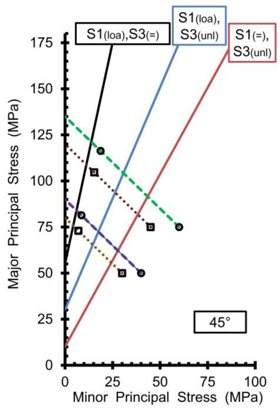
Figure 9.
Stress paths between the initial anisotropic stress state and the linear elastic calculation of the stress state on the borehole wall for an angle of 45°. The starting points and the stress states at failure are indicated by squares and circles. All information is superimposed on the failure envelopes for the three basic types of stress paths (see Figure 1). Four different anisotropic stress states are studied (each with a different colour), i.e., (30, 50), (40, 50), (45, 75), and (60, 75) MPa.
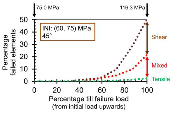
Figure 10.
Variation in the contact failure modes (i.e., tensile-only, shear-only, and mixed modes) as a function of the stress path, i.e., from the initial stress state of (60, 75) MPa till the load level of failure, corresponding to 50% failed contacts. Information is for an angle of 45°.
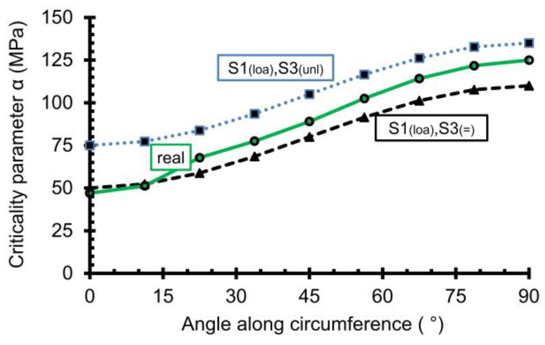
For the initial anisotropic stress state of (60, 75) MPa, the exercise is repeated for all angles along the circumference at 11.25° intervals (Figure 11 and Table 4). The three angles that already have been presented (i.e., 0°, 45°, and 90°) also are included. The stress path for each angle is different because the linear elastic stresses at the circumference are different. This means that the real strength in the approach taken in this study is presented by different points in the major–minor principal stress diagram. Figure 11b presents the stress ranges of interest. In this diagram, the failure envelopes also are drawn for each individual angle. The stress paths starting from the initial anisotropic stress state are not drawn because doing so would overload the graph. For the interval between 45° and 90°, i.e., the most critical zone, the real failure envelopes move away from the type 1 failure envelope (S1(loa),S3(=)) and move towards the type 3 failure envelope (S1(loa),S3(unl)). For an angle of 90°, the “real” strength is closest to the latter for all angles between 0° and 90°. The strength for the angles of 0° and 11.25° are situated close to the type 1 failure envelope. For practical reasons, in the further analysis, it is assumed that the failure envelopes of these two angles are the same as the type 1 failure envelope. In Figure 12, criticality parameter α (Figure 3) is presented as a function of the angle along the circumference. The parameter is presented for the three types of failure envelopes (i.e., type 1, type 3, and the series of the real envelope for each angle). Figure 12 confirms the observations formulated for Figure 11. The curve that corresponds to the real stress paths is closer to the failure envelope of the type 3 stress path for larger angles and further away for smaller angles (and the opposite is true when referring to the type 1 stress path).
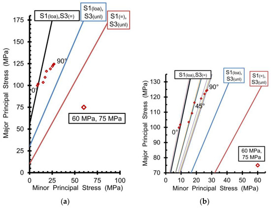
Figure 11.
Strength values following the real stress paths starting from an anisotropic stress state of (60, 75) MPa for all angles along the circumference between 0° and 90° with 11.25° intervals. All information is superimposed on the failure envelopes for the three basic types of stress paths (see Figure 1). (a) Full view; (b) zoomed-in view and all individual failure envelopes added (each with a different colour).
Table 4.
Stress redistribution for the initial anisotropic stress state and parameters describing the criticality of failure along the circumference of the borehole wall, including the minimum mud weight.
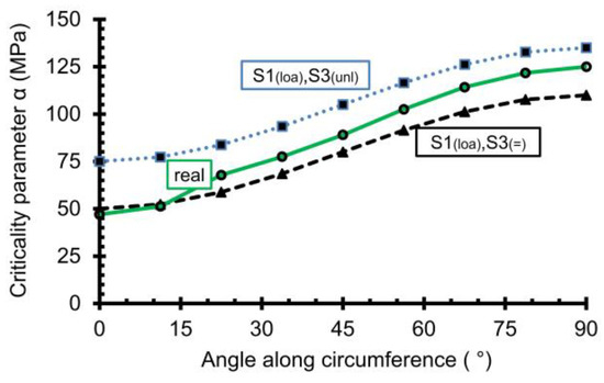
Figure 12.
Variation in criticality parameter α (Figure 3) along circumference of borehole wall for three different stress paths starting from the initial anisotropic stress state of (60, 75) MPa: the real stress path (green), the type 1 stress path (S1(loa),S3(=); black), and the type 3 stress path (S1(loa),S3(unl); blue).
In Table 4, the minimum mud weight is calculated as a function of the angle. Two cases are considered for the initial stress state of (60, 75) MPa. The first case is the case in which the initial major principal stress of 75 MPa corresponds to an approximate depth of 3000 m (Figure 13a). As explained above, this could be a horizontal borehole or a vertical borehole at that depth, whereby the major horizontal principal stress is equal to the vertical (axial) stress. Second is the case in which the initial minor principal stress of 60 MPa corresponds to an approximate depth of 2400 m (Figure 13b). The main reason to consider both depth values is to obtain a good idea about the impact on the critical mud weight.
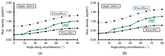
Figure 13.
Variation in the minimum mud density along circumference of borehole wall for three different stress paths starting from the initial anisotropic stress state of (60, 75) MPa: the real stress path (green), the type 1 stress path (S1(loa),S3(=); black) and the type 3 stress path (S1(loa),S3(unl); blue). (a) For a depth of 3000 m; (b) for a depth of 2400 m.
The first observation is that the largest minimum mud weight is needed for the point along the circumference at an angle of 90°. The second observation is that the mud weight for all angles, taking into account the real or in situ stress paths, is situated between the values if one applies the type 1 loading or the type 3 loading and unloading of both principal stresses. The third observation is a confirmation that the difference in mud weights for small angles is small between the real stress paths and the type 1 loading. The fourth observation is linked to the ratio between the minimum mud weight for an angle of 90° and the one for an angle of 0°. For the type 1 loading, this ratio is equal to 2.2 for both depths. However, for the real stress paths, this ratio is about 3 (i.e., 2.9 for an assumed depth of 3000 m and 3.5 for 2400 m). The latter value is equal to 1.261 kg/dm3 divided by 0.333 kg/dm3 (Table 4). Although one could say that the only relevant value is the overall largest minimum weight of mud, which is applied along the entire circumference, the variation in the individual calculated values along the circumference gives a good idea about the critical arc. This leads to the fifth observation, when, for example, for a depth of 2400 m, one looks at the arc where a minimum mud weight of 1 kg/dm3 is needed. For the real stress path, this arc corresponds to angles between about 56° and 90°. However, if the rock is characterised by classic laboratory experiments, all values are below a minimum mud weight of 1 kg/dm3.
4. Discussion and Conclusions
Since halfway through the 20th century, the rock mechanical community has been testing intact rock specimens by starting from a zero-stress state and systematically increasing the load. On the one hand, the main goals of these experiments are the determination of the strength of rocks and possibly the entire failure envelope. On the other hand, there is the goal to obtain a better understanding of the fracturing process that leads to the failure of the specimens. However, it is important to admit that we still do not fully understand either the entire process of rock failure at the lab scale or the link with the in situ behaviour of a rock mass. This statement clearly is supported by the numerous research projects that are still being conducted that focus on the basic type of loading applied in laboratory experiments. These projects often focus on a specific aspect, for example, the impact of heterogeneities (e.g., [10,27,28]), the orientations of flaws or weak planes (e.g., [21,29,30,31]), and the characterisation of the (micro-)fracturing process by the analysis of acoustic emission signals (e.g., [15,16,17,32,33]). These are only a few of the many examples that use classic testing procedures. The correct characterisation of the rock strength and a good understanding of the failure process are essential for all types of design, but their importance even has increased because, more and more, the design should integrate the concepts of long-term behaviour and sustainability.
Some researchers have looked at alternative loading, e.g., dynamic loading (e.g., [6,34,35,36,37]), cyclic loading (e.g., [5,6,7]), or even more complex loading paths (e.g., [8,11]), but the focus of these projects is on developing a better understanding of the phenomenon rather than on characterising the strength of a rock and the failure envelope. In this paper, as was the case in the previous publication, the question is whether one would benefit from having a more accurate and more reliable design when the testing procedure of the specimens are changed significantly. As mentioned above, the current laboratory practice starts from a zero-stress state, and this is followed by the loading of the specimen. In situ, the starting point is the in situ stress state and, due to the excavation, this is followed by an unloading or a combination of unloading one stress component and the loading of another. The paper addresses two questions, i.e., (1) has the application of different stress paths during rock characterisation a significant impact on rock strength and the failure envelope; (2) if so, is the impact on the design parameters relevant? In this paper, the latter is the minimum mud weight that is needed to eliminate the fracturing of the rock around a circular borehole.
The answer to the first question clearly is positive, and it also was the conclusion of an earlier publication [4]. The main advantage of numerical simulations and working with the same black box rock RVE is that one can test the same model as often as needed. This is clearly not the case when testing real specimens. Apart from the fact that the amount of available rock material is almost always limited, rock material still is heterogeneous to a certain degree, which means that no two specimens are exactly the same. Also, there is the restrictions of time and cost when conducting experiments. The simulations show that large reductions in the strength of a rock can occur. For example, the reduction in the strength for the uniaxial unloading stress path in comparison to the uniaxial loading stress path is about 40 to 45%. A comparison between the simultaneous loading and unloading stress paths and the uniaxial loading shows a strength reduction of about 30%. These values are obtained when the initial stress state is isotropic. The reduction in the strength is less when the initial stress state is anisotropic.
The answer to the second question also is positive. For an initial isotropic stress state, the minimum density of the mud when characterising the rock by stress paths that are close to the in situ stress variation can be two to three times larger than when the rock is characterised by stress paths that are close to the classic experimental procedures. For the initial anisotropic stress state, the answer remains positive, but the analysis becomes very complex because each point along the circumference undergoes a different stress path. The impact is discussed in detail above, but the main conclusions are as follows: (i) the most critical point along the circumference remains the point with the largest tangential stress; (ii) depending on the input parameters, the minimum mud weight can be up to 60% larger when the stress path is close to the in situ stress path instead of the one close to the classic experiments; (iii) and the arc along the circumference where a minimum mud weight of 1 kg/dm3, for example, is required is larger when the in situ stress path is considered.
The overall conclusion of the analysis presented in this paper is that the impact of different stress paths needs further attention. The characterisation of the strength or the characterisation of the entire failure envelope based on a stress path closer to the in situ stress paths leads to more correct values than if one characterises the rock by loading rock specimens in the classic experiments. Such a significant change in the procedure of rock characterisation will not be realised from one day to the next. It also is logical that further research is needed, e.g., a 3D analysis, a more detailed RVE model, typical in situ stress paths for other applications, and a verification by laboratory experiments. It is only at that moment that one can start thinking about implementing it in the engineering design. However, some of the more complex stress paths, i.e., with a change in principal stress orientations, cannot be implemented easily in a laboratory. After learning more about the impact of different stress paths, one must probably make some choices, one of which is whether such implementations will be possible or whether they would be impractical. However, the combination of laboratory experiments and the simulation of RVE models could become a worthwhile combination. The analysis also highlighted again that discrete models really are needed to study the behaviour of rock material, as the micro-fracturing during nearly the entire variation in the stress state plays an important role. A good next step in the discrete modelling of rock material is to calibrate the models by also using experiments whereby in situ stress paths are applied.
Funding
This research received no external funding.
Institutional Review Board Statement
Not applicable.
Informed Consent Statement
Not applicable.
Data Availability Statement
Data are contained within the article.
Conflicts of Interest
The author declares no conflicts of interest.
References
- Bieniawski, Z.T.; Bernede, M.J. Suggested Methods for Determining the Uniaxial Compressive Strength and Deformability of Rock Materials. Int. J. Rock Mech. Min. Sci. 1979, 16, 138–140. [Google Scholar] [CrossRef]
- European Standard EN1997-2. Eurocode 7, Geotechnical design, Part 2, Ground Investigation and Testing, Chapter 5.14, Strength Testing of Rock Material. 2010. Available online: https://eurocodes.jrc.ec.europa.eu/EN-Eurocodes/eurocode-7-geotechnical-design (accessed on 21 April 2024).
- ASTM D7012-14e1. Standard Test Methods for Compressive Strength and Elastic Moduli of Intact Rock Core Specimens under Varying States of Stress and Temperatures. 2023. Available online: https://www.astm.org/d7012-14e01.html (accessed on 21 April 2024).
- Vervoort, A. Different Stress Paths Lead to Different Failure Envelopes: Impact on Rock Characterisation and Design. Appl. Sci. 2023, 13, 11301. [Google Scholar] [CrossRef]
- Ding, Z.W.; Jia, J.D.; Tang, Q.B.; Li, X.F. Mechanical Properties and Energy Damage Evolution Characteristics of Coal Under Cyclic Loading and Unloading. Rock Mech. Rock Eng. 2022, 55, 4765–4781. [Google Scholar] [CrossRef]
- Ning, Z.; Xue, Y.; Li, Z.; Su, M.; Kong, F.; Bai, C. Damage Characteristics of Granite Under Hydraulic and Cyclic Loading–Unloading Coupling Condition. Rock Mech. Rock Eng. 2022, 55, 1393–1410. [Google Scholar] [CrossRef]
- Zhang, A.; Xie, H.; Zhang, R.; Gao, M.; Xie, J.; Jia, Z.; Ren, L.; Zhang, Z. Mechanical properties and energy characteristics of coal at different depths under cyclic triaxial loading and unloading. Int. J. Rock Mech. Min. Sci. 2023, 161, 105271. [Google Scholar] [CrossRef]
- Li, Y.; Fu, J.; Hao, N.; Song, W.; Yu, L. Experimental study on unloading failure characteristics and damage evolution rules of deep diorite based on triaxial acoustic emission tests. Geosci. J. 2023, 27, 629–646. [Google Scholar] [CrossRef]
- Debecker, B.; Vervoort, A. Two-dimensional discrete element simulations of the fracture behavior of slate. Int. J. Rock Mech. Min. Sci. 2013, 61, 161–170. [Google Scholar] [CrossRef]
- Van Lysebetten, G.; Vervoort, A.; Maertens, J.; Huybrechts, N. Discrete element modeling for the study of the effect of soft inclusions on the behavior of soil mix material. Comput. Geotech. 2014, 55, 342–351. [Google Scholar] [CrossRef]
- Song, Z.; Zhang, J.; Wang, S.; Dong, X.; Zhang, Y. Energy Evolution Characteristics and Weak Structure—“Energy Flow” Impact Damaged Mechanism of Deep-Bedded Sandstone. Rock Mech. Rock Eng. 2023, 56, 2017–2047. [Google Scholar] [CrossRef]
- Itasca, 2004. UDEC v4.0 manual. Itasca Consulting Group, Inc. 2004. Available online: https://www.itascacg.com/software/udec (accessed on 21 April 2024).
- Dong, L.J.; Chen, Y.C.; Sun, D.Y.; Zhang, Y.H.; Deng, S.J. Implications for identification of principal stress directions from acoustic emission characteristics of granite under biaxial compression experiments. J. Rock Mech. Geotech. Eng. 2023, 15, 852–863. [Google Scholar] [CrossRef]
- Ganne, P.; Vervoort, A.; Wevers, M. Quantification of pre-peak brittle damage: Correlation between acoustic emission and observed micro-fracturing. Int. J. Rock Mech. Min. Sci. 2007, 44, 720–729. [Google Scholar] [CrossRef]
- Chang, S.H.; Lee, C.I. Estimation of cracking and damage mechanisms in rock under triaxial compression by moment tensor analysis of acoustic emission. Int. J. Rock Mech. Min. Sci. 2004, 41, 1069–1086. [Google Scholar] [CrossRef]
- Du, K.; Li, X.; Tao, M.; Wang, S. Experimental study on acoustic emission (AE) characteristics and crack classification during rock fracture in several basic lab tests. Int. J. Rock Mech. Min. Sci. 2020, 133, 104411. [Google Scholar] [CrossRef]
- Liu, X.; Zhang, H.; Wang, X.; Zhang, C.; Xie, H.; Yang, S.; Lu, W. Acoustic Emission Characteristics of Graded Loading Intact and Holey Rock Samples during the Damage and Failure Process. Appl. Sci. 2019, 9, 1595. [Google Scholar] [CrossRef]
- Cundall, P.A. A computer model for simulating progressive large-scale movements in block rock systems. In Proceedings of the ISRM Symposium, Nancy, France, 4–6 September 1971. Paper II-8. [Google Scholar]
- Fjær, E.; Holt, R.M.; Horsrud, P.; Raaen, A.M.; Risnes, R. (Eds.) Petroleum Related Rock Mechanics. In Developments in Petroleum Science, 2nd ed.; Elsevier: Amsterdam, The Netherlands, 2008; Volume 53, 491p, ISBN 978-0-444-50260-5. [Google Scholar] [CrossRef]
- Xiang, Z.; Moon, T.; Oh, J.; Si, G.; Canbulat, I. Analytical investigations of in situ stress inversion from borehole breakout geometries. J. Rock Mech. Geotech. Eng. 2023; in press. [Google Scholar] [CrossRef]
- Zhang, Y.; Long, A.; Zhao, Y.; Zang, A.; Wang, C. Mutual impact of true triaxial stress, borehole orientation and bedding inclination on laboratory hydraulic fracturing of Lushan shale. J. Rock Mech. Geotech. Eng. 2023, 15, 3131–3147. [Google Scholar] [CrossRef]
- Wang, S.; Liao, G.; Zhang, Z.; Wang, X. Study on Wellbore Stability Evaluation Method of New Drilled Well in Old Reservoir. Processes 2022, 10, 1334. [Google Scholar] [CrossRef]
- Deangeli, C.; Omwanghe, O.O. Prediction of Mud Pressures for the Stability of Wellbores Drilled in Transversely Isotropic Rocks. Energies 2018, 11, 1944. [Google Scholar] [CrossRef]
- Shi, Y.; Ma, T.; Zhang, D.; Chen, Y.; Liu, Y.; Deng, C. Analytical model of wellbore stability analysis of inclined well based on the advantageous synergy among the five strength criteria. Geofluids 2023, 2023, 2201870. [Google Scholar] [CrossRef]
- Lavrov, A.; Vervoort, A.; Wevers, M.; Napier, J.A.L. Experimental and numerical study of the Kaiser effect in cyclic Brazilian tests with disk rotation. Int. J. Rock Mech. Min. Sci. 2002, 39, 287–302. [Google Scholar] [CrossRef]
- Eberhardt, E. Numerical Modelling of Three-Dimension Stress Rotation Ahead of an Advancing Tunnel Face. Int. J. Rock Mech. Min. Sci. 2001, 38, 499–518. [Google Scholar] [CrossRef]
- Malan, D.F.; Napier, J.A.L. Computer modelling of granular material microfracturing. Tectonophysics 1995, 248, 21–37. [Google Scholar] [CrossRef]
- Van de Steen, B.; Vervoort, A.; Sahin, K. Influence of internal structure of crinoidal limestone on fracture paths. Int. J. Eng. Geol. 2002, 67, 109–125. [Google Scholar] [CrossRef]
- Wang, T.; Ye, W.; Liu, L.; Li, A.; Jiang, N.; Zhang, L.; Zhu, S. Impact of Crack Inclination Angle on the Splitting Failure and Energy Analysis of Fine-Grained Sandstone. Appl. Sci. 2023, 13, 7834. [Google Scholar] [CrossRef]
- Chang, X.; Zhang, X.; Dang, F.; Zhang, B.; Chang, F. Failure Behavior of Sandstone Specimens Containing a Single Flaw Under True Triaxial Compression. Rock Mech. Rock Eng. 2022, 55, 2111–2127. [Google Scholar] [CrossRef]
- Van de Steen, B.; Vervoort, A.; Napier, J.A.L.; Durrheim, R.J. Implementation of a flaw model to the fracturing around a vertical shaft. Rock Mech. Rock Eng. 2003, 36, 143–161. [Google Scholar] [CrossRef]
- Dong, L.; Zhang, Y.; Bi, S.; Ma, J.; Yan, Y.; Cao, H. Uncertainty investigation for the classification of rock micro-fracture types using acoustic emission parameters. Int. J. Rock Mech. Min. Sci. 2023, 162, 105292. [Google Scholar] [CrossRef]
- Xie, N.; Tang, H.M.; Yang, J.B.; Jiang, Q.H. Damage Evolution in Dry and Saturated Brittle Sandstone Revealed by Acoustic Characterisation Under Uniaxial Compression. Rock Mech. Rock Eng. 2022, 55, 1303–1324. [Google Scholar] [CrossRef]
- Hu, L.; Yu, L.; Ju, M.; Li, X.; Tang, C. Effects of intermediate stress on deep rock strainbursts under true triaxial stresses. J. Rock Mech. Geotech. Eng. 2023, 15, 659–682. [Google Scholar] [CrossRef]
- Du, K.; Tao, M.; Li, X.B.; Zhou, J. Experimental study of slabbing and rockburst induced by true-triaxial unloading and local dynamic disturbance. Rock Mech. Rock Eng. 2016, 49, 3437–3453. [Google Scholar] [CrossRef]
- Gong, F.Q.; Wu, C.; Luo, S.; Yan, J.Y. Load–unload response ratio characteristics of rock materials and their application in prediction of rockburst proneness. Bull. Eng. Geol. Environ. 2019, 78, 5445–5466. [Google Scholar] [CrossRef]
- Liu, D.; Sun, J.; Li, R.; He, M.; Cao, B.; Zhang, C.; Meng, W. Experimental study on the effect of unloading rate on gneiss rockburst. J. Rock Mech. Geotech. Eng. 2023; in press. [Google Scholar] [CrossRef]


Disclaimer/Publisher’s Note: The statements, opinions and data contained in all publications are solely those of the individual author(s) and contributor(s) and not of MDPI and/or the editor(s). MDPI and/or the editor(s) disclaim responsibility for any injury to people or property resulting from any ideas, methods, instructions or products referred to in the content. |
© 2024 by the author. Licensee MDPI, Basel, Switzerland. This article is an open access article distributed under the terms and conditions of the Creative Commons Attribution (CC BY) license (https://creativecommons.org/licenses/by/4.0/).