Abstract
Research on evaluating sustainable transport policies is predominantly focused on their urban effects, often overlooking similar challenges in suburban and rural mobility. Therefore, the development of regionally integrated sustainable transport strategies becomes essential to comprehensively address these concerns. This study aims to bridge this gap by introducing a GIS-supported methodology that combines multiple linear regressions with hazard ratio models to quantify and map the impacts of environmentally driven regional transport policies on air pollution and human health. The main findings of an illustrative case study highlighted the importance of stronger efforts to promote the transition to shared and active transport and address the articulation between urban and rural mobility. This study offers a novel contribution to transport researchers and policymakers by proposing a methodology that (1) forecasts the impacts of regional transport policies using open data and software, ensuring its applicability for diverse regional settings, (2) provides the results in quantitative and visual formats, facilitating output analysis and visualisation and, consequently, decision-making and public consultation on proposed sustainable transport policies, and (3) sets the groundwork for including future transport-related dimensions.
1. Introduction
Transport-sourced pollutants, such as nitrogen oxides (NOx) and particulate matter (PM2.5 and PM10), are continually released into the atmosphere [1] and epidemiological cohort studies have found associations between long-term exposure to these outdoor air pollutants and mortality [2,3]. Even though concentrations have decreased in the past decade, research suggests that the health effects may persist at the current lowered levels, indicating there may be benefits in further reducing exposure to these pollutants [4,5].
Therefore, it is just as important to track the impacts of transport-sourced variations in NOx and PM emissions on human health as the emissions that lead to global climate change [6]. These may be linked to changes in vehicle technology [7] or in the implementation of transport systems, encouraging the use of less-polluting modes of travel [8].
Reducing the use of private motorised vehicles in conjunction with promoting the use of active and public transportation is essential to meet emission targets and improve public health [9]. These forms of transportation can have additional impacts, which should be considered when estimating the overall impacts of transport on human health, such as the exercise benefits of active travel [10] and the reduction in traffic collisions [11].
Previous studies investigating the links between transport policy changes and health outcomes [8,12,13] focused on urban transport since these areas hold higher population densities and, therefore, increased potential for large-scale emission reductions and health improvements [14]. However, this broadens an existing research gap by excluding suburban and rural areas, where people are often left with no choice other than to rely on privately owned vehicles, due to the lack of adequate sustainable transport alternatives [15].
Quantum Geographic Information Systems (QGIS) is an open-access mapping software commonly used for viewing, manipulating, and complex spatial analysis across different geographic levels [16]. This multifaceted software has been applied in different areas, including transportation [17,18] and health [19] studies. Furthermore, it has also been acknowledged as a powerful resource for supporting the impact analysis and forecasting of transportation projects [20,21].
Therefore, with an understanding of the value of developing regionally integrated transport strategies [22], this research aims to understand how to facilitate the analysis and optimisation of their environmental and health impacts. This will be fulfilled with the introduction of a location-independent methodology, supported by the following steps:
- Use of open-access data sources and software to ensure diverse regional applications and future updates.
- Development of transport-sourced air pollution and human health analytical models using established modelling and statistical principles.
- Application of geospatial methods in QGIS to generate mapped distributions of those impacts across a region.
- Testing an illustrative regional case study to understand the required data inputs and potential outcomes of the methodology.
This research provides a novel contribution to the transportation research and policymaking fields with the proposal of a methodology that can be replicated for multiple regional case studies and allows for future updates. Additionally, providing the outputs in quantitative and mapping formats facilitates data analysis, visualisation, decision-making, and public consultation processes concerning proposed sustainable transport policies.
2. Materials and Methods
This study was conducted using publicly available data and software so that the approach could be easily replicated for other regions. The data sources (Table 1) and methodology are described in this section, as well as the sensitivity analysis conducted to account for the existing variability in the data. Where possible, existing modelling techniques were used, with a preference towards approaches and data from official government or leading international organisations, such as the World Health Organisation (WHO).

Table 1.
Input data required to map regionally distributed emissions and human health.
2.1. Transport Scenarios
To demonstrate the outcomes of this methodology, three transport scenarios (Table 2) were simulated. These were adapted from the future transport policies devised by the West of England Combined Authority (WECA) [34] and the integrated local authorities of Bath and North East Somerset (BANES) [35], Bristol [36], and South Gloucestershire [37].
Table 2.
Simulated scenarios based on WECA’s future transport strategies.
The initial two scenarios in Table 2 matched the objectives outlined in the gathered transport strategies. The modal-shift scenario seeks to reduce the number of passenger cars by 15%, while simultaneously increasing cycling and bus use by 8% and 6%, respectively. The electrification scenario demonstrates the intention of electrifying 66% of passenger cars and buses. The combined policies scenario aims to merge the previous two scenarios, considering the population distribution between urban and rural areas in the region.
The scenarios in Table 2 were initially simulated with the support of QGIS by applying the following changes to the baseline scenario:
- Multiply the initial number of vehicles in each Average Annual Daily Flow (AADF) georeferenced count point by the corresponding change (%) in the number of vehicle trips.
- Multiply the modal shifts (%) by the associated baseline regional distance travelled per transport mode.
- Multiply the baseline number of cycling trips in the region by the respective change (%).
- Calculate exhaust emissions for petrol and diesel vehicles, by multiplying the initial number of vehicles by the complementary percentage of the one assigned to electrification for both NOx and PM2.5.
- When simulating an electrification scenario, specific emissions factors are adopted for PM2.5 sourced from tyre and brake wear and road abrasion [27], due to electric vehicles being heavier than their petrol and diesel counterparts [38].
2.2. Emissions
To avoid the effects of COVID-19 and mitigate any inaccurate conclusions that might arise from the changes in travel patterns, an illustrative case study was simulated using information from the year 2019.
The calculation of traffic-related emissions was supported by the principles established by the European Environment Agency [39] and widely utilised in the literature [40,41,42,43]. This methodology estimates emissions (E) from:
- Vehicles in grammes per kilometre driven, in this case using the geographically distributed vehicle count points for the AADF.
- Emission factors (EF) in grammes per kilometre.
- The distribution of each propulsion technology and vehicle type (passenger cars, bicycles, motorcycles, buses, light-goods vehicles, and heavy-goods vehicles) in the overall vehicle fleet (FW), as demonstrated in (1):
Secondly, following a similar principle to that in [44], the average annual concentrations for NOx and PM2.5 in µgm−3 across the WECA region were estimated through multiple linear regression models, with the modelled background pollution data for both pollutants (Table 1) used as the dependent variable and the traffic-related emissions and population density as independent variables. The models resulting from this process (Equations (2) and (3)) are functions of the calculated emissions (E) and population density (Pop.Dens) in residents per hectare:
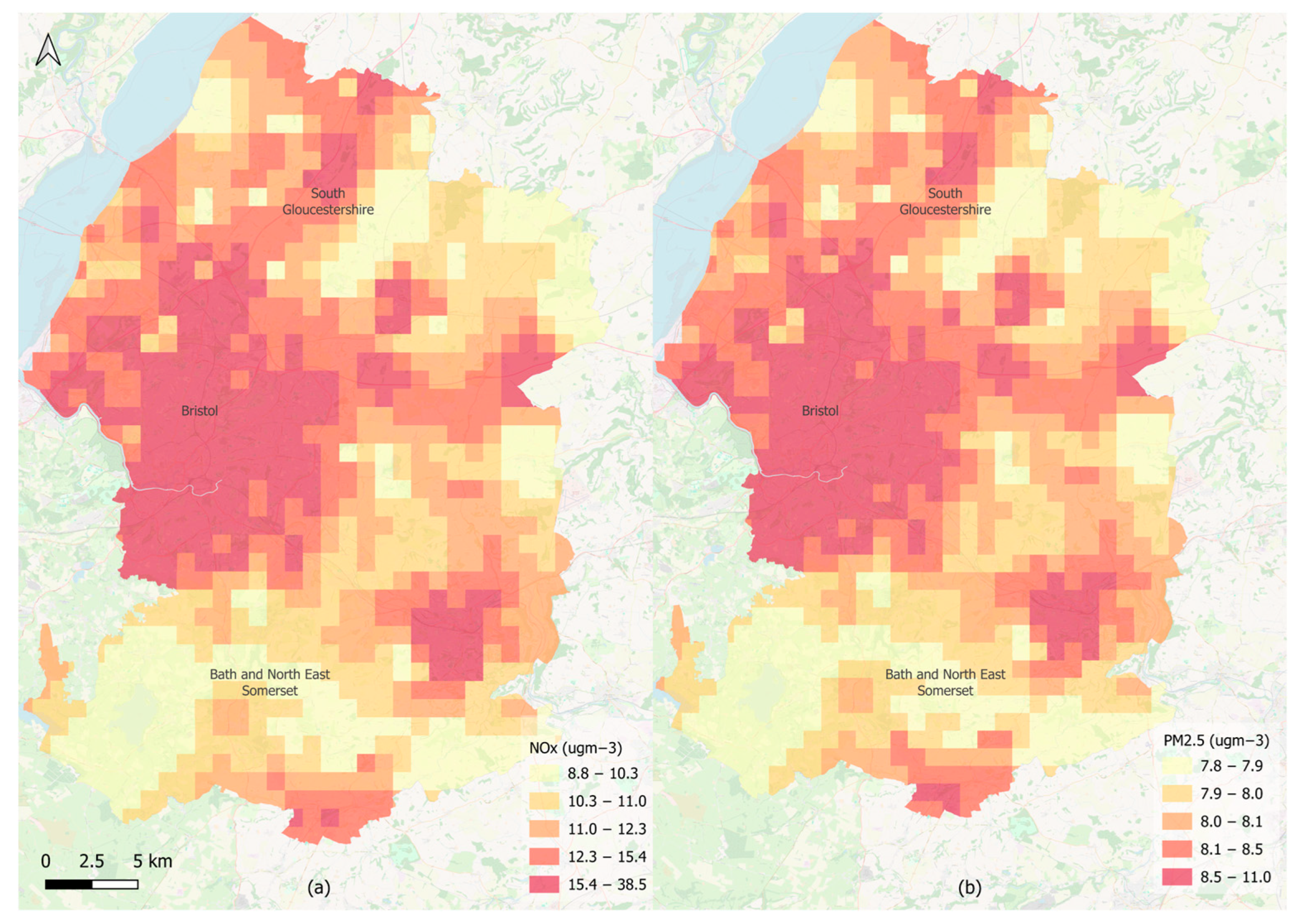
After estimating both pollutants’ average annual concentrations for each AADF count point, an Inverse Distance Weighted (IDW) interpolation was used in QGIS to calculate their distribution over the study area. This produced an emissions grid, where each 1 × 1 km square had an assigned mean concentration value for each pollutant (Figure 1). The developed grid supported the remaining calculations.
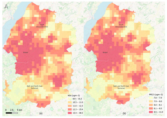
Figure 1.
Grid maps for baseline traffic (a) NOx and (b) PM2.5 emissions (base maps were obtained through OpenStreetMap under a Data Commons Open Database License).
2.3. Health Impacts
The human health impacts were represented as the mortality balance from an intervention, influenced by air pollution, active travel, and fatal traffic collisions.
Formula (4) summarises the framework developed for estimating the transport-related annual mortality , distributed over the developed 1 × 1 km regional square grid, for a given scenario x (Sx) from Table 2. This used the base scenario mortality () and an exponential function of the logarithmic (ln) values for the hazard ( and ) and risk ratios (RR) multiplied by the variations in (1) pollutant concentration ( and ) and (2) cycling volume. The values for collision fatalities from the different transport modes () were added to the previous elements, as shown in Equation (4):
2.3.1. Base Mortality
The distributed baseline mortality in each 1 × 1 km square () was estimated using the total number of annual deaths in the region () multiplied by a ratio of the annual population in each square () and the regional population (), as shown in expression (5):
2.3.2. Emission-Based Mortality
Public health researchers estimate the impacts of emissions on mortality using hazard ratios (HR) obtained through proportional hazard regression models [45]. Since the case study used to demonstrate this methodology was in the UK, the values proposed by the Committee on the Medical Effects of Air Pollutants [46] were applied (Table 3) for this specific demonstration. These values are the result of meta-analyses of existing literature reviews on all-cause mortality related to outdoor air pollution [47].
Table 3.
HRs for increments of 10 µgm−3 of PM2.5 and NOx [47].
2.3.3. Cycling-Based Mortality
The benefits of cycling were estimated with the support of the principles provided in the Health Economic Assessment Tool [33] for cycling. Expression (6) multiplies the logarithmic value of RR () by a ratio of the variation in the local cycling volume in the region () and the reference cycling volume:
To calculate the variation in the local cycling volume (7), the total annual regional cycling trips () were multiplied by the estimated average trip length () and by 60 to match the units in the reference volume (in minutes per week). This was then divided by the total population in the region (), multiplied by an estimated average cycling speed () and by 52 to match the reference volume. Lastly, to distribute the cycling values across the region, these results were multiplied by a population density ratio using the density in each 1 × 1 km square in QGIS () and the total annual regional population density ():
2.3.4. Traffic Collision-Based Mortality
Collision-based mortality was calculated by adapting the principles in [48] using the developed 1 × 1 km grid in QGIS. The RR for traffic collisions () developed in (8) was defined based on the annual mortality and the change in fatalities per vehicle type from Sx to S0 (), which were then normalised using the baseline regional mortality:
The change in fatal collisions (9) was estimated as the variation between Sx and S0 of the fatality rate per vehicle type in deaths per billion vehicle kilometres travelled (), multiplied by the number of vehicle kilometres travelled per vehicle type ():
The final number of collision-based fatalities () was calculated, as shown in (10), by multiplying the mortality in each 1 × 1 km square by the attributable fraction of the mortality among the exposed population () using the previously determined RR (11):
2.4. Sensitivity Analysis
Following the example of other research and transport studies [48,49], a Monte Carlo simulation was conducted to assess the variability and associated uncertainty of the model. For this research, the input parameters were determined to have the distributions shown in Table 4, with each 1 × 1 km cell having different input parameters and assigned variable distributions (see the Supplementary Materials).
Table 4.
Input variables and associated distribution parameters.
The Monte Carlo simulation involves randomly choosing a probability value and sample across each variable and square for 10,000 runs. Due to the nature of the analysis and data, a few steps in the process must be noted:
- The inputs for NOx and PM2.5 emissions resulted from regression models, therefore, each value in one 1 × 1 km square in the grid had an individual 95% confidence interval associated with a normal distribution (see the Supplementary Materials).
- The correlation between emissions and the associated HR was mitigated by assigning different random probability values for each distribution.
3. Results and Discussion
3.1. Emissions
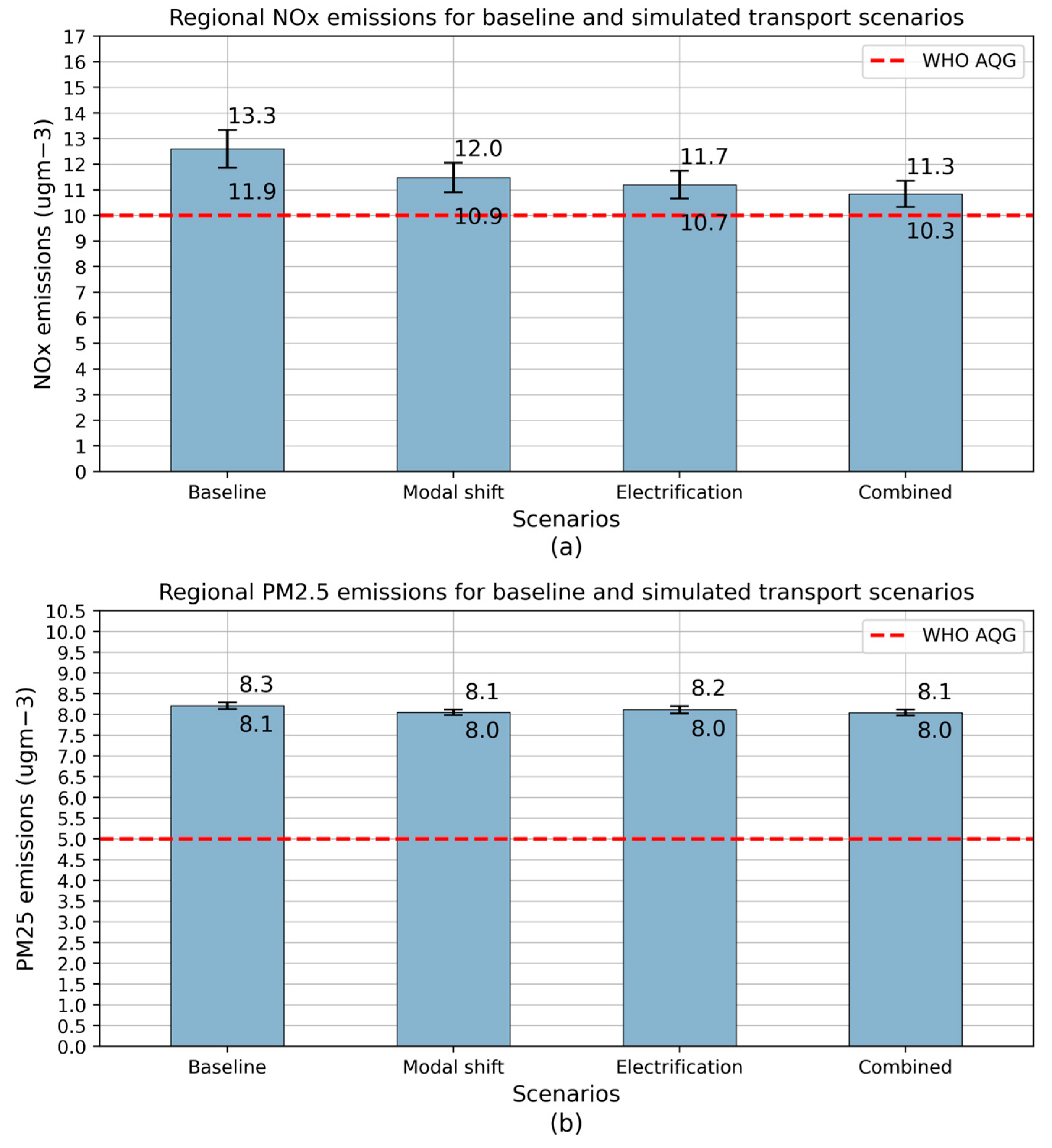
Figure 2 shows the NOx (plot (a)) and PM2.5 (plot (b)) reductions across the illustrative future policy scenarios in Table 2, including the baseline scenario. The figure also displays the health-advised Air Quality Guidelines (AQG) recommended by the WHO [50].
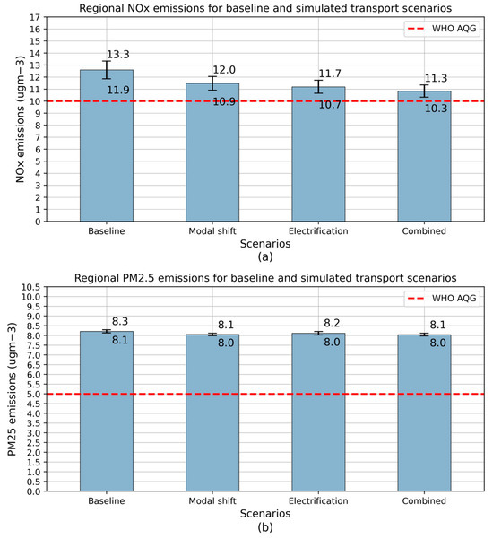
Figure 2.
Average regional NOx (a) and PM2.5 (b) concentrations for the baseline and simulated scenarios, with 95% confidence limits and the AQG recommended by the WHO [50].
The comparison between the modal-shift-only and electrification-driven policies highlighted the latter as having the highest reduction in NOx (around 1.5 µgm−3). This can be explained by (1) the main source for NOx being exhaust pollution, which is eliminated for electric vehicles, and (2) the increase in the number of buses as a result of the modal-shift scenario, since these are heavier vehicles and will, therefore, lead to higher NOx emissions.
Nevertheless, encouraging the use of shared and active transport closely followed the NOx reduction (1.1 µgm−3) achieved with electrification, since this behavioural change encompasses a decrease in the number of cars on the road, mitigating the impact on emissions coming from these vehicles.
The combined policies scenario contributed to the highest reductions in NOx, from 12.6 for the baseline scenario to approximately 10.8 µgm−3. Even though it involves efforts in changing travelling behaviour, hence increasing the number of buses on the road, the investments of 66% in the electrification of the remaining private cars and the increased number of buses further enhance the efforts in reducing NOx concentrations. Overall, these findings showed that individual investments in electrification or changes from cars to buses and bicycles did not achieve the same level of benefits as a combined approach, which would optimise the effects of reducing NOx emissions.
Plot (a) in Figure 2 indicates that the annual average NOx emissions produced in the region for all the planned transport policy scenarios are still not enough to meet the stricter WHO AQG, with the combined scenario producing annual emissions that were still 0.8 µgm−3 above that guideline. Even though the simulated policies maintained emissions under the UK target of 40 µgm−3 [51], this was already complied with in a baseline scenario where no changes were implemented.
PM2.5 (plot (b)) is also produced from exhaust sources, but the main source is tyre and brake wear, as well as road abrasion. This clarifies why a move focused only on electrification had higher effects on NOx emissions but lower reductions for PM2.5 (from 8.2 to 8.1 µgm−3) when compared to all the other scenarios. On the other hand, the two policy scenarios entailing modal shift revealed enhanced potential for reducing annual PM2.5, with average regional reductions towards approximately 8.0 µgm−3.
Comparing the annual average PM2.5 emissions with the AQG from the WHO emphasised, once again, that none of the illustrative future transport scenarios have the potential to reduce this pollutant’s concentration below the AQG of 5 µgm−3.
Overall, these results strengthen the rationale for using a methodology that facilitates the development of regional transport strategies prioritising an adequate balance between promoting modal shift and vehicle electrification considering their impacts on local air quality.
3.2. Human Health
The regional human health effects of all these scenarios were determined by the avoided premature mortality, expressed as the number of lives saved, due to changes in emissions, cycling activity, and fatal traffic collisions. Figure 3 displays the cumulative probability functions for the expected avoided mortality, revealing the probabilities for each scenario to save up to a certain number of lives.

Figure 3.
Probability functions for regional mortality across the simulated scenarios.
Overall, the electrification scenario stood out as the policy that was less likely to reduce mortality, with a mean of 110 lives saved regionally and a 97.5% chance of increasing that to 200 lives. This substantiates that the strategy centred on electrification was far from meeting the potential achieved from policies focused only on modal shifts, where an average of 240 lives could be saved and there was a 97.5% probability of extending that number to 320. However, the combination of electrification and modal shift escalated the number of lives saved to almost 300, with a 97.5% probability of increasing to 410 lives.
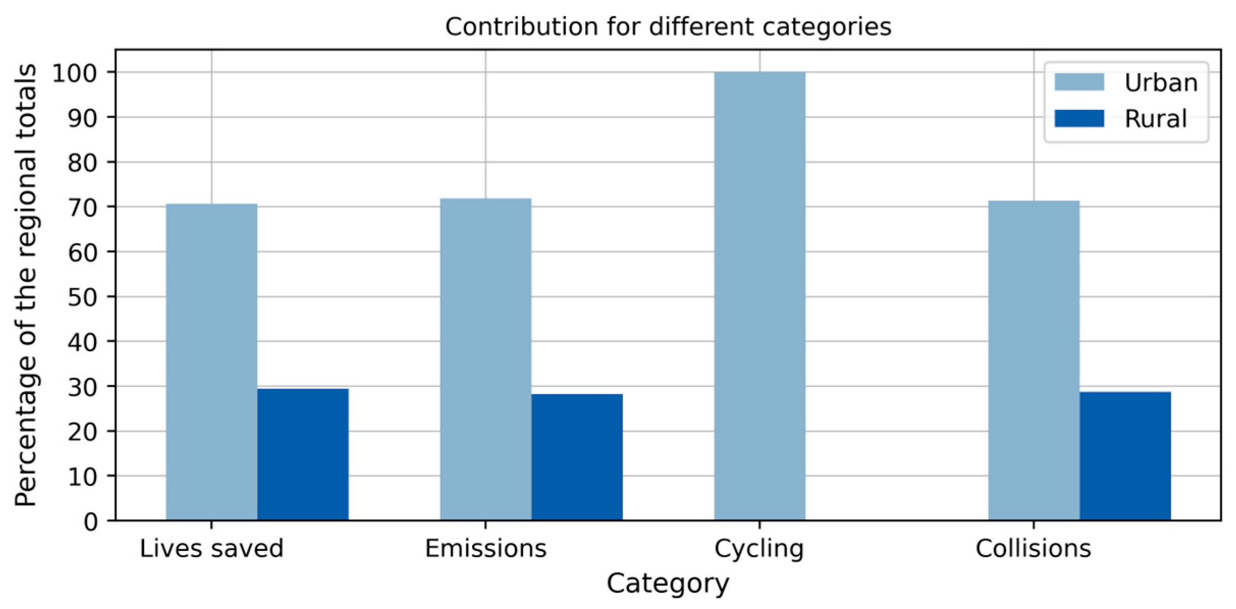
Furthermore, this methodology enabled the development of Figure 4, which depicts the contribution of transport-related factors in the mortality calculations, including the effects of changes in air pollutant concentrations, cycling activity, and fatal traffic collisions.
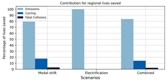
Figure 4.
Transport-related contributions to regional human health impacts.
Figure 4 provides evidence supporting the reason why a modal-shift-only scenario could be responsible for saving more lives on average than an electrification-only strategy:
- As opposed to an electrification scenario, modal shift contributed to higher reductions in PM2.5, which had a higher contribution to reducing human mortality than NOx.
- The stimulation of cycling activity enhanced the health benefits of exercise.
- The reduction in the use of private cars and the move towards bus use contributed to lower fatal traffic collisions.
Concerning the contributions from each factor, in an electrification-driven policy scenario, 100% of the lives saved came from the reduction in air pollution, as it was the only factor changing in the model. On the other hand, the policy focused only on modal shift exhibited a distribution of around 79%, 18%, and 3% for the improvements in emissions, fatal traffic collisions, and cycling, respectively, therefore leading to a higher number of lives saved.
The combined policies scenario emphasised the complexity of designing future regional policies since it accumulated an increased number of lives saved, with similar contributions to the modal-shift-only scenario, with around 84%, 14%, and 2% for emissions, cycling, and collisions, respectively. However, this scenario could potentially involve higher investments (e.g., infrastructure provision), as it includes both the modal shift and electrification efforts.
This methodology assisted in maximising the benefits of these transport policies, by providing the outputs linked to the specific transport-related element (emissions, cycling, or collisions), hence pinpointing the areas where improvement is required.
3.3. Urban and Rural Areas
A regional approach should differentiate between urban and rural areas when equally distributing and assessing the impacts of these strategies on emissions and human health. Here, the combined policies scenario (Table 2) stood out for targeting a real-world characterisation of how these changes would impact densely and sparsely populated areas.
Figure 5 presents the proportion of urban and rural areas among the regional values for the human health impacts of the combined policies scenario. Rural areas included the 1 × 1 km squares in the QGIS grid with population densities of up to 21 residents per hectare, and the urban areas were those including densities between 21 and 115 residents per hectare.

Figure 5.
Urban-rural distribution of the health impacts resulting from the combined policies scenario.
The modal-shift percentages distributed for the urban-rural areas in the combined policies scenario led to a few anticipated results, such as the 6% increase in cycling only in urban areas (Table 2), where this mode of transportation is preferred for short-distance and last-mile trips, leading to health benefits centred in urban areas. Another example was the distribution of the 8% regional increase (Table 2) in bus use while guaranteeing access to these services in sparsely populated regions. This change most likely led to a higher proportion of prevented deaths from traffic collisions in rural areas (28.7%), as shown in Figure 5.
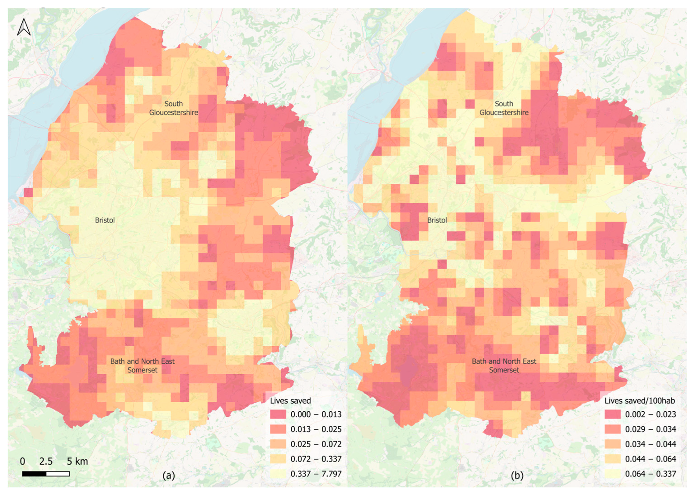
The geographical distribution of human health impacts in the combined scenario (Figure 6a) highlighted urban areas as having higher numbers of avoided premature mortality when compared to rural areas. To minimise the potential imbalance of the results due to higher population densities in urban environments, the number of lives saved in each square was adjusted by dividing it by the population numbers in each 1 × 1 km square (Figure 6b). Although this adjustment slightly enhanced the mortality rates in rural areas, it did not eliminate the disparities between these two scales, which were consistent with the findings in Figure 5.
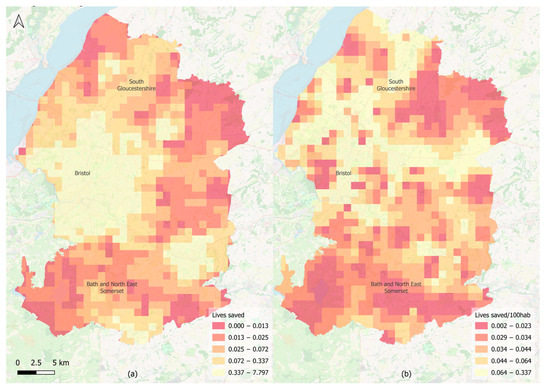
Figure 6.
Total lives saved per 1 × 1 km cell (a) and lives saved per 100 habitants (b) when implementing the combined policies scenario (base maps were obtained through OpenStreetMap under a Data Commons Open Database License).
These expected results helped to validate the outputs generated by this methodology and emphasised the advantages of its use to facilitate the development of regional policies focused on equitably balancing the distributed benefits of future modal shift and electrification goals.
3.4. Limitations and Policy Recommendations
One of the limitations of this study is related to the data used, specifically, the assumption of traffic flow and vehicle counts as equal measures for directly applying the modal-shift percentages. Additionally, the study considered an even regional distribution of the mortality risk ratios, which simplified the existing geographical and demographic variability of these hazard ratios.
Secondly, the established methodology was restricted to assessing the effects on human health solely within a specified geographical region, excluding any impacts arising from emissions originating outside this region, even though they could potentially be contributing to changes within the defined boundaries. This is the case for the energy used for charging or producing electric vehicles. Another example is the long-term health impacts of climate change resulting from CO2 emissions, which were not considered, as these cannot be accurately determined with a closed boundary area.
These limitations emphasise the need for governmental cooperation on national and regional levels to develop integrated and standardised strategies and policies aimed at mitigating the adverse impacts of mobility while considering the cross-boundary effects on other regions and industrial sectors. Furthermore, local authorities should incorporate these strategies and collect the needed data with a level of granularity that enhances the accuracy of the outcomes generated from these methodologies.
The illustrative case study provided evidence supporting the need for policymakers to define more ambitious regional modal-shift and electrification goals while addressing the distinct transportation needs in urban and rural areas. This is crucial for efficiently allocating resources and financial investments across these scales to enhance transportation environmental and health equity. The proposed methodology can actively contribute to this by enabling (1) the simulation of individual and combined effects of regional transport policies, and (2) the optimisation of policy goals, considering their equitable distribution in urban and rural areas.
This research provided a geographically flexible methodology for transport policymakers to estimate and visualise the distribution of local emissions and human health effects resulting from regional transport policies. The ability to deliver the outputs in both quantitative and graphical formats enables efficient data analysis, visualisation, and dissemination, therefore ensuring transparency in decision-making processes.
4. Conclusions
This research developed a GIS-supported methodology to estimate and map the geographically distributed air pollution and health impacts of regional transport policies, using the WECA region as an illustrative case study to demonstrate its potential applications and output formats.
The results from the case study confirmed that prioritising investments in multimodal transport incentives and regional integration could decrease transport emissions and contribute towards reductions in premature mortality, whether through the reduction in emissions and traffic collisions or the benefits of active travel.
Furthermore, the research substantiated the potential for this methodology to assist in the development of strategic transport policies aimed at reducing the localised effects of air pollution and enhancing health benefits while considering the diversity between urban and rural contexts.
The novelty of this research lies in the development of a location-independent approach, supported by open-source software and data. This allows future regional applications, enabling policymakers to quantify the human health impacts of transport policies and map their distribution across the region, which could be valuable during consultation and implementation stages as a tool to inform the relevant sectors.
Supplementary Materials
The following supporting information can be downloaded at: https://www.mdpi.com/article/10.3390/su16114728/s1.
Author Contributions
Conceptualisation, R.P.F., A.H. and N.M.; methodology, R.P.F., A.H., N.M. and T.S.; investigation, R.P.F., A.H. and N.M.; data collection, R.P.F.; writing—original draft preparation, R.P.F.; writing—review and editing, R.P.F., A.H., N.M. and T.S.; visualisation, R.P.F., A.H., N.M. and T.S.; supervision, A.H. and N.M. All authors have read and agreed to the published version of the manuscript.
Funding
Rita Prior Filipe is supported by a scholarship from the EPSRC Centre for Doctoral Training in Advanced Propulsion Systems (AAPS), under the project EP/S023364/1.
Institutional Review Board Statement
Not applicable.
Informed Consent Statement
Not applicable.
Data Availability Statement
Data is contained within the article or Supplementary Materials.
Acknowledgments
This study is part of the doctoral research of the first author, conducted at the Department of Architecture and Civil Engineering, University of Bath, under the supervision of the second and third authors. For the purpose of open access, the authors have applied a Creative Commons Attribution (CC-BY) licence to any Author-Accepted Manuscript version arising.
Conflicts of Interest
The authors declare no conflicts of interest.
References
- (European Environmental Agency) EEA. EEA Signals 2013: Every Breath We Take—Improving Air Quality in Europe. 2013. Available online: https://www.eea.europa.eu/publications/eea-signals-2013 (accessed on 20 November 2022). [CrossRef]
- Beelen, R.; Raaschou-Nielsen, O.; Stafoggia, M.; Andersen, Z.J.; Weinmayr, G.; Hoffmann, B.; Wolf, K.; Samoli, E.; Fischer, P.; Nieuwenhuijsen, M.; et al. Effects of long-term exposure to air pollution on natural-cause mortality: An analysis of 22 European cohorts within the multicentre ESCAPE project. Lancet 2014, 383, 785–795. [Google Scholar] [CrossRef] [PubMed]
- Brunekreef, B.; Strak, M.; Chen, J.; Andersen, Z.J.; Atkinson, R.; Bauwelinck, M.; Bellander, T.; Boutron, M.C.; Brandt, J.; Carey, I.; et al. Mortality and Morbidity Effects of Long-Term Exposure to Low-Level PM(2.5), BC, NO(2), and O(3): An Analysis of European Cohorts in the ELAPSE Project. Res. Rep. Health Eff. Inst. 2021, 2021, 1–127. [Google Scholar] [PubMed]
- Cohen, A.J.; Brauer, M.; Burnett, R.; Anderson, H.R.; Frostad, J.; Estep, K.; Balakrishnan, K.; Brunekreef, B.; Dandona, L.; Dandona, R.; et al. Estimates and 25-year trends of the global burden of disease attributable to ambient air pollution: An analysis of data from the Global Burden of Diseases Study 2015. Lancet 2017, 389, 1907–1918. [Google Scholar] [CrossRef] [PubMed]
- Festy, B. Review of evidence on health aspects of air pollution—REVIHAAP Project. Technical Report; World Health Organization: Copenhagen, Denmark, 2013; pp. 1–132. [Google Scholar]
- West, J.J.; Smith, S.J.; Silva, R.A.; Naik, V.; Zhang, Y.; Adelman, Z.; Fry, M.M.; Anenberg, S.; Horowitz, L.W.; Lamarque, J.-F. Co-benefits of mitigating global greenhouse gas emissions for future air quality and human health. Nat. Clim. Chang. 2013, 3, 885–889. [Google Scholar] [CrossRef]
- SRavi, S.S.; Osipov, S.; Turner, J.W.G. Impact of Modern Vehicular Technologies and Emission Regulations on Improving Global Air Quality. Atmosphere 2023, 14, 1164. [Google Scholar] [CrossRef]
- Labee, P.; Rasouli, S.; Liao, F. The implications of Mobility as a Service for urban emissions. Transp. Res. Part D Transp. Environ. 2021, 102, 103128. [Google Scholar] [CrossRef]
- Woodcock, J.; Edwards, P.; Tonne, C.; Armstrong, B.G.; Ashiru, O.; Banister, D.; Beevers, S.; Chalabi, Z.; Chowdhury, Z.; Cohen, A.; et al. Public health benefits of strategies to reduce greenhouse-gas emissions: Urban land transport. Lancet 2009, 374, 1930–1943. [Google Scholar] [CrossRef]
- Kelly, P.; Kahlmeier, S.; Götschi, T.; Orsini, N.; Richards, J.; Roberts, N.; Scarborough, P.; Foster, C. Systematic review and meta-analysis of reduction in all-cause mortality from walking and cycling and shape of dose response relationship. Int. J. Behav. Nutr. Phys. Act. 2014, 11, 132. [Google Scholar] [CrossRef]
- Chandrasekharan, A.; Nanavati, A.J.; Prabhakar, S.; Prabhakar, S. Factors Impacting Mortality in the Pre-Hospital Period After Road Traffic Accidents in Urban India. Trauma Mon. 2016, 21, e22456. [Google Scholar] [CrossRef]
- Borrego, C.; Tchepel, O.; Barros, N.; Miranda, A. Impact of road traffic emissions on air quality of the Lisbon region. Atmos. Environ. 2000, 34, 4683–4690. [Google Scholar] [CrossRef]
- DRojas-Rueda, D.; de Nazelle, A.; Tainio, M.; Nieuwenhuijsen, M.J. The health risks and benefits of cycling in urban environments compared with car use: Health impact assessment study. BMJ 2011, 343, d4521. [Google Scholar] [CrossRef] [PubMed]
- Fragkias, M.; Lobo, J.; Strumsky, D.; Seto, K.C. Does Size Matter? Scaling of CO2 Emissions and U.S. Urban Areas. PLoS ONE 2013, 8, e64727. [Google Scholar] [CrossRef] [PubMed]
- Velaga, N.R.; Beecroft, M.; Nelson, J.D.; Corsar, D.; Edwards, P. Transport poverty meets the digital divide: Accessibility and connectivity in rural communities. J. Transp. Geogr. 2012, 21, 102–112. [Google Scholar] [CrossRef]
- Rosas-Chavoya, M.; Gallardo-Salazar, J.L.; Lopez-Serrano, P.M.; Alcantara-Concepcion, P.C.; Leon-Miranda, A.K. QGIS a Constantly Growing Free and Open-Source Geospatial Software Contributing to Scientific Development. Cuad. Investig. Geogr. 2022, 48, 197–213. [Google Scholar] [CrossRef]
- Campisi, T.; Russo, A.; Tesoriere, G.; Al-Rashid, M.A. A Two-Steps Analysis of the Accessibility of the Local Public Transport Service by University Students Residing in Enna BT—Computational Science and Its Applications—ICCSA 2023 Workshops; Gervasi, O., Murgante, B., Rocha, A.M.A.C., Garau, C., Scorza, F., Karaca, Y., Torre, C.M., Eds.; Springer Nature: Cham, Switzerland, 2023; pp. 147–159. [Google Scholar]
- Soldatke, N.; Sydorów, M.; Żukowska, S. Assessment of the accessibility of public transport in the Tricity (Poland): Analytical use of geographical information systems (GIS) in the context of selected public transport measures. Int. J. Digit. Earth 2024, 17, 2344586. [Google Scholar] [CrossRef]
- Kim, J.; Kim, D.H.; Lee, J.; Cheon, Y.; Yoo, S. A scoping review of qualitative geographic information systems in studies addressing health issues. Soc. Sci. Med. 2022, 314, 115472. [Google Scholar] [CrossRef] [PubMed]
- Fortunato, G.; Scorza, F.; Murgante, B. Cyclable City: A Territorial Assessment Procedure for Disruptive Policy-Making on Urban Mobility BT—Computational Science and Its Applications—ICCSA 2019; Misra, S., Gervasi, O., Murgante, B., Stankova, E., Korkhov, V., Torre, C., Rocha, A.M.A.C., Taniar, D., Apduhan, B.O., Tarantino, E., Eds.; Springer International Publishing: Cham, Switzerland, 2019; pp. 291–307. [Google Scholar]
- Wilches-Mogollon, M.A.; Sarmiento, O.L.; Medaglia, A.L.; Montes, F.; Guzman, L.A.; Sánchez-Silva, M.; Hidalgo, D.; Parra, K.; Useche, A.F.; Meisel, J.D.; et al. Impact assessment of an active transport intervention via systems analytics. Transp. Res. Part D Transp. Environ. 2024, 128, 104112. [Google Scholar] [CrossRef]
- Allard, R.F.; Moura, F. The Incorporation of Passenger Connectivity and Intermodal Considerations in Intercity Transport Planning. Transp. Rev. 2016, 36, 251–277. [Google Scholar] [CrossRef]
- ONS. Census 2021 Geographies. Available online: https://www.ons.gov.uk/methodology/geography/ukgeographies/censusgeographies/census2021geographies (accessed on 10 December 2022).
- ONS. Population Estimates by Output Areas, Electoral, Health and Other Geographies, England and Wales. Available online: https://www.ons.gov.uk/peoplepopulationandcommunity/populationandmigration/populationestimates/bulletins/annualsmallareapopulationestimates/mid2020 (accessed on 5 December 2022).
- DfT. Estimated Motor Vehicle Traffic per Local Authority. Available online: https://roadtraffic.dft.gov.uk/local-authorities (accessed on 9 November 2022).
- NAEI. Emissions Factors for Transport. Available online: https://naei.beis.gov.uk/data/ef-transport (accessed on 30 November 2022).
- Beddows, D.C.S.; Harrison, R.M. PM10 and PM2.5 emission factors for non-exhaust particles from road vehicles: Dependence upon vehicle mass and implications for battery electric vehicles. Atmos. Environ. 2021, 244, 117886. [Google Scholar] [CrossRef]
- Defra. Modelled Background Pollution Data. Available online: https://uk-air.defra.gov.uk/data/pcm-data (accessed on 30 November 2022).
- OS. OS Open Roads. Available online: https://www.ordnancesurvey.co.uk/products/os-open-roads (accessed on 11 September 2022).
- DfT. National Travel Survey: 2019. Available online: https://www.gov.uk/government/statistics/national-travel-survey-2019 (accessed on 30 November 2022).
- DfT. Reported Road Casualties Great Britain, Annual Report: 2019. Available online: https://www.gov.uk/government/statistics/reported-road-casualties-great-britain-annual-report-2019 (accessed on 20 November 2022).
- ONS. Deaths Registered by Area of Usual Residence, UK. Available online: https://www.ons.gov.uk/peoplepopulationandcommunity/birthsdeathsandmarriages/deaths/datasets/deathsregisteredbyareaofusualresidenceenglandandwales (accessed on 15 November 2022).
- WHO. Health Economic Assessment Tool (HEAT) for Walking and for Cycling. WHO, no. December. p. 73. 2017. Available online: http://www.euro.who.int/__data/assets/pdf_file/0010/352963/Heat.pdf?ua=1%0Ahttps://www.euro.who.int/en/health-topics/environment-and-health/Transport-and-health/publications/2017/health-economic-assessment-tool-heat-for-walking-and-for-cycling.-methods-an (accessed on 20 November 2023).
- West of England Combined Authority. Joint Local Transport Plan 4; West of England Combined Authority: Bristol, UK, 2020. [Google Scholar]
- Bath & North East Somerset Council. Transport Delivery Action Plan for Bath; Bath & North East Somerset Council: Bath, UK, 2020.
- Bristol Council. Bristol Transport Strategy; Bristol Council: Bristol, UK, 2019.
- South Gloucestershire Council. Local Transport Plan (2020–2041); South Gloucestershire Council: Bristol, UK, 2020; p. 235. [Google Scholar]
- Timmers, V.R.J.H.; Achten, P.A.J. Non-exhaust PM emissions from electric vehicles. Atmos. Environ. 2016, 134, 10–17. [Google Scholar] [CrossRef]
- Ntziachristos, L.; Samaras, Z.; Gorißen, N. COPERT III Computer Programme to Calculate Emissions from Road Transport Methodology and Emission Factors (Version 2.1) with Contributions from. 2000. Available online: http://www.eea.eu.int (accessed on 20 November 2022).
- Carroll, P.; Caulfield, B.; Ahern, A. Measuring the potential emission reductions from a shift towards public transport. Transp. Res. Part D Transp. Environ. 2019, 73, 338–351. [Google Scholar] [CrossRef]
- Federico, G.; Ferrante, P.; Lascari, G.; Sorrentino, G.; Traverso, M. A Simplified Method for the Environmental Impact of Urban Transportation. In Proceedings of the 4th International SIIV Congress, Palermo, Italy, 12–14 September 2007; p. 135. Available online: http://www.siiv.net/site/sites/default/files/Documenti/palermo/63_2848_20080110105953.pdf (accessed on 20 October 2022).
- Mcnamara, D.G. Capping Transport Emissions: A Welfare Analysis of a Personal Carbon Trading Scheme. 2012. Available online: http://www.tara.tcd.ie/handle/2262/76232?show=full (accessed on 20 November 2022).
- Soylu, S. Estimation of Turkish road transport emissions. Energy Policy 2007, 35, 4088–4094. [Google Scholar] [CrossRef]
- Beelen, R.; Hoek, G.; Vienneau, D.; Eeftens, M.; Dimakopoulou, K.; Pedeli, X.; Tsai, M.-Y.; Künzli, N.; Schikowski, T.; Marcon, A.; et al. Development of NO2 and NOx land use regression models for estimating air pollution exposure in 36 study areas in Europe—The ESCAPE project. Atmos. Environ. 2013, 72, 10–23. [Google Scholar] [CrossRef]
- Cox, D.R. Regression Models and Life-Tables. J. R. Stat. Society. Ser. B Methodol. 1972, 34, 187–220. [Google Scholar] [CrossRef]
- Summary of COMEAP recommendations for the quantification of health effects associated with air pollutants. Available online: https://assets.publishing.service.gov.uk/media/64fadfdea78c5f0014265847/COMEAP_Quantification_recommendations.pdf (accessed on 20 November 2022).
- Chen, J.; Hoek, G. Long-term exposure to PM and all-cause and cause-specific mortality: A systematic review and meta-analysis. Environ. Int. 2020, 143, 105974. [Google Scholar] [CrossRef] [PubMed]
- Rojas-Rueda, D.; de Nazelle, A.; Teixidó, O.; Nieuwenhuijsen, M. Replacing car trips by increasing bike and public transport in the greater Barcelona metropolitan area: A health impact assessment study. Environ. Int. 2012, 49, 100–109. [Google Scholar] [CrossRef]
- Guimarães, V.d.A.; Junior, I.C.L.; da Silva, M.A.V. Evaluating the sustainability of urban passenger transportation by Monte Carlo simulation. Renew. Sustain. Energy Rev. 2018, 93, 732–752. [Google Scholar] [CrossRef]
- WHO. WHO Global Air Quality Guidelines. Particle Matter (PM2.5 and PM10), Ozone, Nitrogen Dioxide, Sulfur Dioxide and Carbon Monoxide; WHO: Geneva, Switzerland, 2021.
- A.I.R. UK AIR. UK Air Quality Limits. Available online: https://uk-air.defra.gov.uk/air-pollution/uk-limits.php (accessed on 21 March 2024).


Disclaimer/Publisher’s Note: The statements, opinions and data contained in all publications are solely those of the individual author(s) and contributor(s) and not of MDPI and/or the editor(s). MDPI and/or the editor(s) disclaim responsibility for any injury to people or property resulting from any ideas, methods, instructions or products referred to in the content. |
© 2024 by the authors. Licensee MDPI, Basel, Switzerland. This article is an open access article distributed under the terms and conditions of the Creative Commons Attribution (CC BY) license (https://creativecommons.org/licenses/by/4.0/).