Article

Synergistic Evolution of PM2.5 and O3 Concentrations: Evidence from Environmental Kuznets Curve Tests in the Yellow River Basin

1
College of Geography and Environment, Shandong Normal University, Jinan 250358, China
2
Key Research Institute of Yellow River Civilization and Sustainable Development & Collaborative Innovation Center on Yellow River Civilization, Henan University, Kaifeng 475001, China
3
International Department, Shandong Experimental High School, Jinan 250116, China
*
Authors to whom correspondence should be addressed.
These authors contributed equally to this work.
Sustainability 2024, 16(11), 4744; https://doi.org/10.3390/su16114744
Submission received: 22 April 2024 / Revised: 28 May 2024 / Accepted: 31 May 2024 / Published: 2 June 2024
(This article belongs to the Section Air, Climate Change and Sustainability)

Abstract

:
Air pollution, especially the synergistic pollution of PM2.5 and O3, poses a severe threat to human life and production. The synergistic formation mechanism of PM2.5 and O3 pollution is relatively confirmed, while research on their spatiotemporal synergy is urgent. Based on remotely sensed interpretation data from 90 cities in the Yellow River Basin, we analyzed the synergistic evolution of PM2.5 and O3 concentrations during 2013–2020. Combined with the environmental Kuznets curve, we performed factor analysis using a panel regression model. The synergistic evolution pattern shows a gradual decrease in PM2.5 concentration and a gradual increase in O3 concentration. There is a strong spatial auto-correlation in the two pollutants’ concentrations. The relationship between economy and PM2.5 concentration shows an “N-shaped” curve, while that between O3 concentration and economic development presents an inverse “N-shaped” curve. The environmental Kuznets curve shows that the deterioration of O3 pollution takes place later than the mitigation of PM2.5 pollution. Various factors have obvious heterogeneous effects on PM2.5 and O3 concentrations. Meanwhile, the sensitivity effect of per capita GDP on PM2.5 concentration in the midstream region is stronger than that in the upstream region, while the sensitivity effect of per capita GDP on O3 concentration is strongest in the midstream region than that in upstream and downstream region.

1. Introduction

With the implementation of a series of environmental regulations in China, PM2.5 pollution has been significantly improved [1]. However, O3 concentration has been increasing gradually [2], and the phenomenon of PM2.5–O3 synergistic pollution has appeared increasingly prominent [3,4]. PM2.5–O3 synergistic pollution is due to the fact that the two have the same precursors (NOx and VOCs) [5], which generate O3 through photochemical reactions under light conditions and interact with PM2.5 through transmission and diffusion, aerosol processes, and cloud processes, ultimately forming regional synergistic pollution [6]. Existing studies have sufficiently confirmed that exposure to PM2.5–O3 has increased the possibility of respiratory [7] and cardiovascular diseases [8] and led to the decline in some crop yields, resulting in economic losses [9]. This has also become a severe constraint [10] on sustainable urban construction [11]. Therefore, the latest policy, which was formulated in China in 2023, takes the mitigation of PM2.5 concentration as a key breakthrough and vigorously decreases NOx and VOCs concentration to synergize the amelioration of PM2.5–O3 pollution.
The existing literature on PM2.5 and O3 has mainly concentrated on source analysis [12,13], synergistic mechanisms [14,15], single-pollutant and multipollutant spatiotemporal evolution [16,17,18], spatial correlation [19], and factor studies [20,21]. PM2.5 sources are relatively complex—partially primary emissions (primary particulate matter) and partially secondary formation (secondary particulate matter) [22]. Primary PM2.5 mainly originates from human production through the consumption of fossil energy and other forms of emission [23]. Secondary particulate matter is mainly produced from the transformation of gaseous precursors (including NOx and NH3) emitted into the atmosphere [24] during industrial production, transportation, and other processes. NOx and VOCs produce most of the ground-level O3 through photochemical reactions [5]. Ground-level O3 is also affected by weather conditions, such as rainfall [25]. Existing studies on synergistic mechanisms have confirmed that PM2.5 and O3 are homologous pollutants, while NOx and VOCs are common precursors of both [26]. Meanwhile, there is a complex chemical coupling mechanism between the two pollutants, whose relationship will change significantly with the rapid evolution of pollution [27]. Elevated O3 concentrations facilitate atmospheric oxidizability and the generation of components including PM2.5, sulfates, and organic compounds [6]. PM2.5 and O3 concentrations are more often shown to be synergistic [28]. Studies on their spatiotemporal evolution and correlation are also abundant, covering the scales of nations [29], urban agglomerations [30,31], climate zoning [32], provinces [33], and cities [34]. In terms of factors, the main focus is on natural factors—ranging from precipitation [35], vegetation [36], wind speed [37], and per capita GDP [30] to urbanization [38], digital economy [39,40], and other socio-economic factors—to analyze their effects on air pollutant concentrations. The specific factor research methods include GWR [41], machine learning [23,42], GeoDetector [43], and spatial metrics [44].
First of all, most existing studies take air monitoring sites as data sources, and the uneven and sparse distribution of site monitoring data is likely to cause bias in the analysis, making it difficult to fully introduce the distribution of pollutants in the whole study area, along with their influencing mechanisms. Secondly, the current research has mainly focused on the analysis of the temporal variation in a single pollutant (such as daily variation, monthly variation, and seasonal variation). The spatiotemporal variation in PM2.5 and O3 is not discussed. Finally, the research areas are mostly concentrated in economically developed areas, paying little attention to natural watershed areas, and often analyzing the driving factors of a single pollutant at the urban agglomeration or city scale, while ignoring the correlation characteristics of different pollutant-influencing factors, making it difficult to effectively carry out the management of clean air.
Based on the above research deficiencies, we feel that Yellow River Basin (YRB) is a crucial area to study the synergistic evolution of air pollution and the human–land relationship [45]. First of all, this large river basin is one of the regions most strongly influenced by the relationship between humans and land. Due to the particularity of its natural environment and geographical location, the ecological environment of the YRB is always facing great threats [40]. Secondly, the YRB is a national strategic implementation region. The YRB’s application of the western development strategy, industrial transfer, and other policies all have a profound impact on the spatiotemporal patterns of air pollutants [46]. Thirdly, due to the YRB’s tiered development pattern, the socio-economic development of various regions has great heterogeneity. The imbalance and insufficiency within the basin are particularly prominent [47]. Finally, clean air is the comprehensive embodiment of the harmonious relationship between humans and land in the YRB [48]. However, according to the 2023 air quality ranking of 168 key cities, 9 of the bottom 10 and 16 of the bottom 20 cities are distributed in the YRB. Serious air pollution has hindered high-quality development in the YRB [40]. However, there have been few empirical quantitative studies on the synergistic evolution of air pollution in large river basins. Therefore, the YRB was selected as the research area, and the dynamic evolution of PM2.5 and O3 concentrations was investigated with the help of EKCs, which has clear regional typical characteristics and important academic research value.
Hence, we selected remotely interpreted data to analyze the synergistic evolution of PM2.5 and O3 concentrations in YRB during 2013–2020. We aimed to analyze the synergistic evolution patterns and influence mechanisms of PM2.5 and O3 concentrations in the YRB through EKCs, determine whether there was a previous synergistic evolution rule between them, and identify the specific rule to provide a basis for the coordinated management of PM2.5–O3 pollution in the YRB. This is an undoubtedly vital theoretical exploration and empirical study on the harmonious development of the ecology in large river basins, in the hope that our findings can improve the specialized application of sustainable development disciplines.
In this study, we proposed the following two hypotheses:
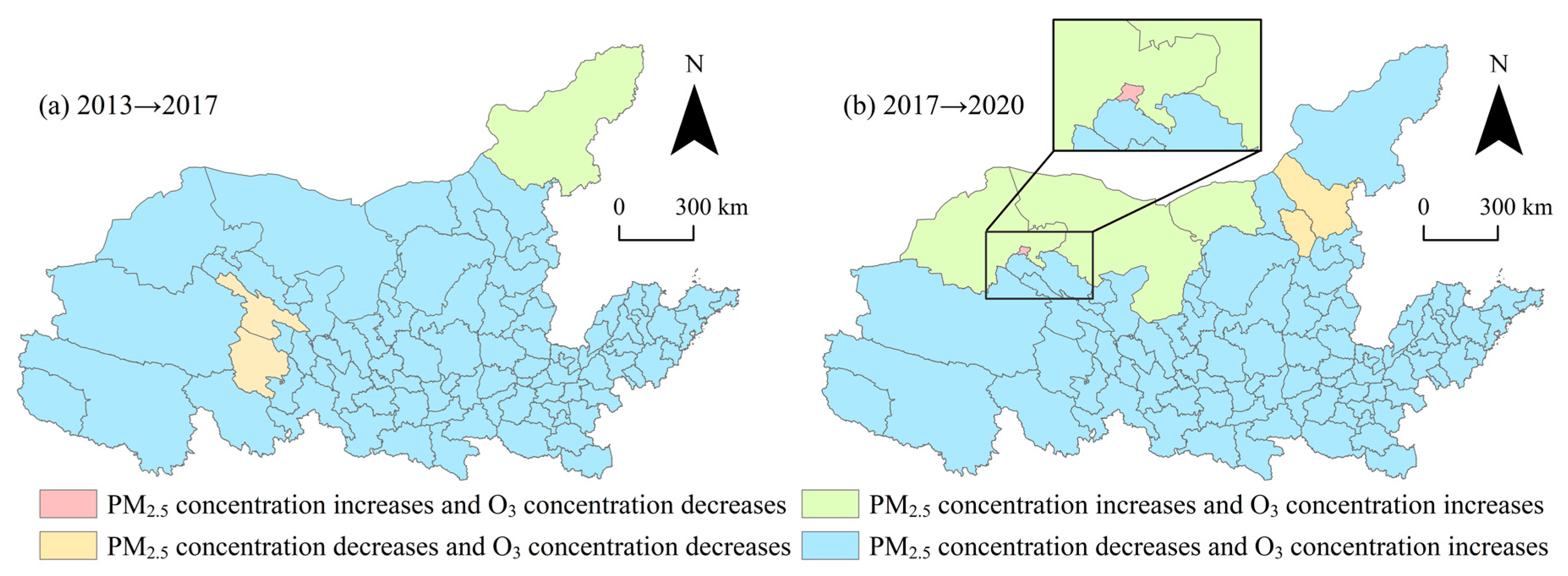
  • There is an obvious synergistic evolution rule of PM2.5 and O3 concentrations.
  • There is a synergistic evolution pattern of decreasing PM2.5 concentration and increasing O3 concentration.

2. Data and Methodology
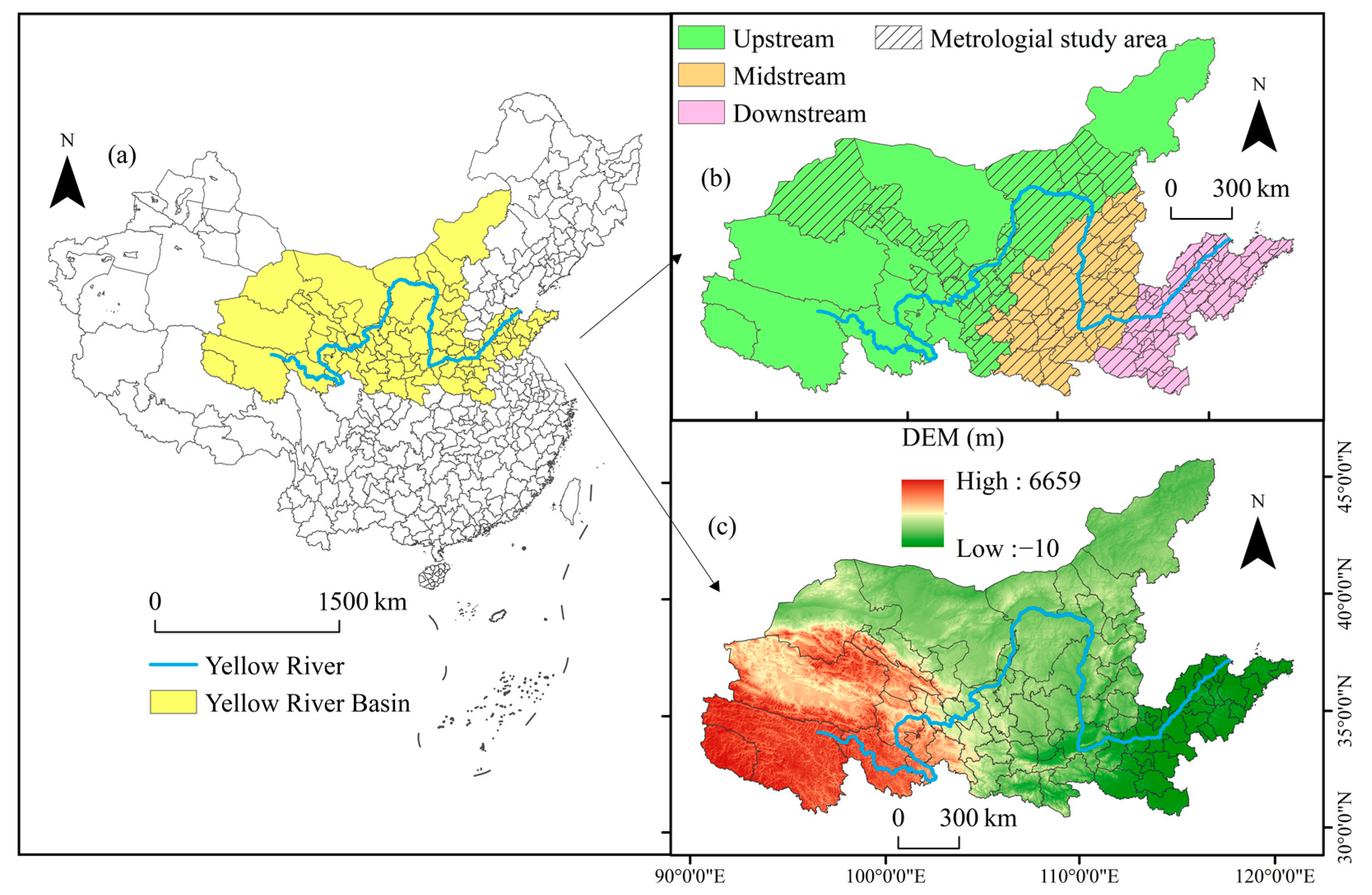
2.1. Study Area

The YRB spans the three terrain steps of China, with complex and diverse ecological types, and is a vital ecological barrier in China [49]. At the same time, the YRB is one of the most important cradles of the Chinese nation and Chinese civilization, rich in energy resources, and a major energy base in China [50]. We focus on the eight provinces through which the Yellow River flows as the main body, fully consider the integrity of important ecosystems, the rationality of resource allocation, and the close connections of the Yellow River, and ensure the integrity of administrative units in the study area as much as possible [51]. The study area is 2.55 million km2; it includes 90 prefecture-level administrative units (Figure 1), accounting for 26.56% of China’s national territorial area. In 2020, the population of the YRB reached 301 million, accounting for 21.3% of China’s total population, which constitute one of the centers of population distribution in China. In 2020, the total GDP in the YRB accounted for 46.8% of China’s northern region, while the per capita GDP was only 59,900 RMB (far lower than China’s per capita GDP of 71,800 RMB), and regional development was extremely uneven.
The 90 prefecture-level administrative units in the YRB include 32 cities in its upstream, 28 cities in its midstream, and 30 cities in its downstream. However, due to differences in the acquisition of socio-economic data, only 78 cities were retained as our study area during the regression analysis. The 12 cities not included in the econometric model are mainly distributed in the upstream area and belong to the ecologically fragile protected areas. The air quality is relatively good, and the proportion of population and economic aggregation is small. In our study, the effect of economic development on air pollution was mainly explored using EKC, and these regions have little impact on the overall research results of the YRB in the regression model. Combined with previous studies [52,53], these 78 cities can better reflect the air pollution and social development of the YRB.

2.2. Methodology

2.2.1. The Standard Deviational Ellipse (SDE)

We chose the SDE to explain the spatial distribution of air pollutant concentration. The SDE can intuitively describe the distribution and multidimensional characteristics of a research object; thus, it can accurately measure the center of gravity, distribution range, shape, and orientation of air pollution concentration in the YRB [54]. The change in the area of the SDE can determine the concentration or dispersion trend. The direction of the axis can describe the main/minor distribution direction of air pollution, and the change in the rotation can reflect the change in the main direction of air pollution distribution. The closer the ratio is to 1, the more radially uniform the air pollution concentration [54]. The center of the SDE represents the center of gravity of air pollutant concentration, and the change trajectory can describe the overall movement trend of air pollutant concentration [32]. The formula of center of air pollutant concentration gravity is:
X ¯ = j = 1 n P t j X t j j = 1 n P t j   Y ¯ = j = 1 n P t j Y t j j = 1 n P t j
where X ¯ and Y ¯ are the longitude and latitude coordinates of the center of gravity, n ∈ [1, …, 90], Ptj is PM2.5 concentration or O3 concentration in city j in year t, while Xtj and Ytj are the longitude and latitude coordinates of the administrative center in city j in year t, t ∈ [2013, …, 2020].

2.2.2. Bivariate Kernel Density Estimation (BKD)

BKD is the kernel density estimation of a two-dimensional random variable, which is a nonparametric test method [55]; it is a kind of distributed dynamic method, which is a nonparametric estimation method for studying regional differences. This method does not presuppose the existence of some functional relationship between economic variables, but it estimates the density function according to the characteristics of the variables themselves, so there is no case that the parameter model cannot fit the data well, meaning that more general conclusions can be drawn [55]. BKD plots are an important method to analyze the joint distribution of two variables, and the dispersion and aggregation characteristics of the two air pollutants can be observed more clearly [56]. By drawing the BKD plots of PM2.5 and O3 concentrations, regional clustering differences and synergistic evolution in the YRB can be discussed.

2.2.3. Bivariate Spatial Auto-Correlation

Bivariate spatial auto-correlation can reveal the spatial cluster association and dependence of two variables [57]. Bivariate global spatial auto-correlation can explore and analyze the spatial correlation between multiple variables and reveal the correlation degree between the PM2.5 concentration of a spatial research unit and the O3 concentration of a neighboring spatial research unit [57]. The formula of bivariate global spatial auto-correlation is:
B M o r a n s   I = a = 1 n b = 1 n W a b ( x a x ¯ ) ( y b y ¯ ) S 2 a = 1 n b = 1 n W i j
where B-Moran’s I is the bivariate global spatial auto-correlation coefficient; n ∈ [1, …, 90]; Wab is the contiguity weight matrix; xa and yb are air pollutant concentration of space units a and b, respectively. x ¯ and y ¯ are averages concentration. The variance of all the samples is S2.
Bivariate local spatial auto-correlation can reflect the agglomeration and spatial differentiation between PM2.5 concentration in each spatial attribute unit and O3 concentration in adjacent units. The specific spatial research units of attribute spatial aggregation and anomalies can be obtained by using the bivariate LISA cluster graph of bivariate local spatial auto-correlation [57]. The formula as follows:
I a = Z a b = 1 n W a b Z b
where Ia is the bivariate local spatial auto-correlation for city a; Za and Zb are the variance standardized values for city a and city b. Z-Score standardization is applied to the indicator data to eliminate the effect of the magnitude in the analysis of bivariate spatial auto-correlation.

2.2.4. Factor Analysis Based on Environmental Kuznets Curves (EKCs)

Based on the Kuznets curve, Grossman and Krueger studied the correlation with environment and economy [58]. The basic principle of the EKC is as follows: the higher the level of initial economic development, the higher the environmental pollution. When economic development reaches a certain stage, economic growth will inhibit environmental quality in inverse proportion [58]. At present, EKCs have been broadly used in environmental economic research, especially for measuring the correlation between air pollution and economy [32].
We selected PM2.5 and O3 concentrations as the core explanatory variables, along with GDP per capita, and quadratic and cubic terms were used to verify the EKC. Air pollution is affected by economic development, industrialization [39] and urbanization [56]. So as to maintain the validity of the model estimates, we chose several control variables. In terms of social and economic factors, we chose the population urbanization rate and population density to characterize urbanization development, and we chose the index of industrial sophistication to measure the effect of industrial upgrading. In previous studies, natural environment has been shown to have a direct impact on air pollutant concentrations [35,36,37]. Vegetation cover [36] and rainfall [35] have a positive effect on air pollution, and air ventilation affects the transfer and diffusion of air pollutants [37]. Therefore, we selected NDVI, precipitation, and ventilation coefficients as control variables.
The correlation between economy and air pollution is deeply analyzed with EKC. For various sub-watersheds, the regression models we constructed also have significant differences. The panel regression model is:
ln P a b = α 1 ln V G D P + α 2 ln 2 V G D P + α 3 ln 3 V G D P + λ a X a + σ + μ
where Pit represents PM2.5 concentration or O3 concentration of region a in year b, i ∈ [1, …, 90], VGDP represents per capita GDP, and air pollutant concentration and per capita GDP are selected to construct the differentiated EKC regression models. Xa represents control variables, such as population urbanization rate and population density. σ is the constant, and μ is the random error. αi is the coefficient to be estimated and determines the shape of EKC (Table 1). We aimed to summarize the synergistic evolution model of PM2.5 and O3 concentrations by using the shape and inflection point of the EKC and the spatiotemporal evolution in the YRB.

2.3. Data Processing and Sources

The data that we used mainly included air pollution concentration data, socio-economic data, and natural environment data. The definition and sources of the specific data are shown in Table 2. We used ArcGIS10.8 for data format conversion, grid tailoring, and zonal statistics to acquire the PM2.5 and O3 concentration datasets. The original socio-economic data were sourced from the Provincial Statistical Yearbook (2014–2021) for each of the eight provinces in the YRB, from which the per capita GDP was directly obtained. The population urbanization rate (urban population/total population), population density (total population/administrative unit area), and the index of industrial sophistication (the ratio of tertiary industry to secondary industry) were obtained via simple calculation. The NDVI and annual average precipitation were interpreted and extracted using ArcGIS10.8. We calculated the ventilation coefficients as described by Hering and Poncet [59].

3. Results

3.1. Spatiotemporal Evolution of PM2.5 and O3 Concentrations

3.1.1. Temporal Trends

A fluctuating downward of PM2.5 concentration was apparent in the YRB during 2013–2020, which was a decrease of 23.56% (Figure 2). PM2.5 concentration showed fluctuating decreases in all sub-watersheds, while its concentration levels and decrease in magnitude varied. PM2.5 concentration decreased abruptly in the mid-downstream regions, with the midstream concentration decreasing from 49.44 μg/m3 to 32.31 μg/m3 (34.65%), and it fell below the secondary limit (35 μg/m3) of the PM2.5 concentration in the Chinese Ambient Air Quality Standard (GB3095-2012) for the first time in 2020. PM2.5 concentration in the downstream decreased the most, from 74.83 μg/m3 to 46.25 μg/m3—a reduction of 25.58 μg/m3, or 38.19%—but was still above the secondary limit. The Action Plan for Prevention and Control of Air Pollution, promulgated in 2013, and the Three-Year Action Plan for Winning the Battle of Defending the Blue Sky, promulgated in 2018, significantly reduced the air pollution. With the reductions in environmental regulations and the gradual recovery of economic activities—especially the output of metallurgy and petrochemicals—pollution in the downstream of the YRB increased compared with previous years, so the PM2.5 concentration in the downstream increased slightly in 2015 and 2019. O3 concentration showed a sharp upward in the YRB during 2013–2019, showing only a slight decrease in 2020 due to the COVID-19 pandemic. O3 concentration increased by 20.52 μg/m3 in the YRB during 2013–2020. The O3 concentration in the upstream, midstream, and downstream areas were generally consistent with the trend in the whole basin, with increases of 17.62%, 29.78%, and 24.92%, respectively. The Theil index of PM2.5 concentration presented a rapid decline from 0.796 to 0.434 during 2013–2020, demonstrating that the regional heterogeneity was gradually decreasing. Nevertheless, the O3 concentration gap between cities was not significant, while the Theil index was at a low level in the YRB. The temporal evolution pattern reflected PM2.5 concentration showed a fluctuating increase, while O3 concentration presented a fluctuating decrease in the YRB.

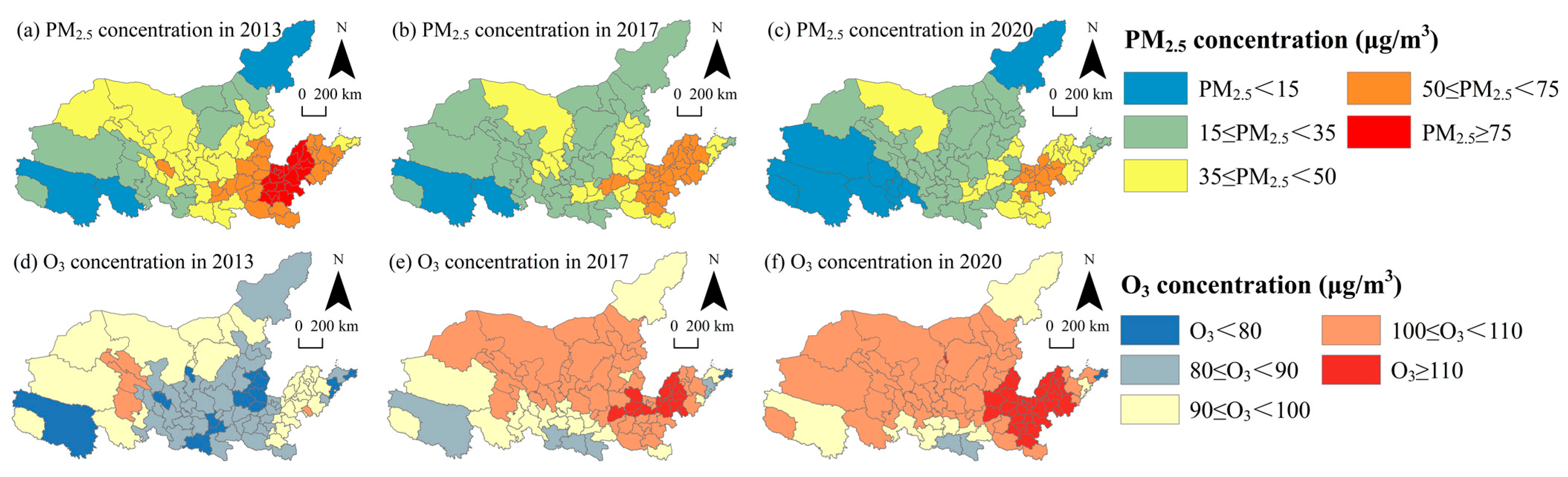
3.1.2. Spatial Distribution

The main policy implementation period of the Action Plan for Prevention and Control of Air Pollution was 2013–2017, while that of the Three-Year Action Plan for Winning the Battle of Defending the Blue Sky was 2018–2020. Therefore, we chose 2017 as the node to observe the distribution patterns of air pollutant concentration in these two periods. There were 76 cities with PM2.5 concentrations exceeding 35 μg/m3 in 2013 (Figure 3a), where those cities with a concentration of 35–50 μg/m3 were located in the up-midstream, while those with a concentration of 50–75 μg/m3 were located in Henan, Shandong, etc. PM2.5 concentration was the highest in Hebi (91.46 μg/m3). There were 18 cities with a PM2.5 concentration above 75 μg/m3 in the downstream region. Those cities with PM2.5 concentrations exceeding the secondary limit (35 μg/m3) in the Ambient Air Quality Standard (GB3095-2012) were mainly located in the mid-downstream and resource-oriented cities in 2017, such as Shizuishan and Wuhai (Figure 3b), and there was only one city (Alashan) in the upstream region with a PM2.5 concentration exceeding the secondary limit (35 μg/m3) in 2020. In 2020, there remained only nine cities in the midstream with PM2.5 concentrations exceeding 35 μg/m3. However, there were 14 cities with PM2.5 concentrations above 50 μg/m3, mostly clustered in the downstream region, including Kaifeng, Puyang, and Heze. O3 concentration was at a relatively high level in the YRB in 2013. Cities with O3 concentrations lower than 80 μg/m3 included Yangquan, Lanzhou, Jinzhong, and Qingdao. Those cities with O3 concentrations higher than 100 μg/m3 included Zhangye and Jiayuguan. Only Weihai had an O3 concentration less than 80 μg/m3 in 2017. O3 concentrations in Inner Mongolia, Ningxia, Shaanxi, and Shanxi generally exceeded 100 μg/m3, while those in some cities in Henan and Shandong exceeded 110 μg/m3 in 2017. Two major agglomeration areas of O3 concentration were formed. The high-value cluster areas with O3 concentrations exceeding 110 μg/m3 covered western Shandong and eastern Henan. There were three cities with O3 concentrations below 90 μg/m3: Weihai, Hanzhong, and Ankang.

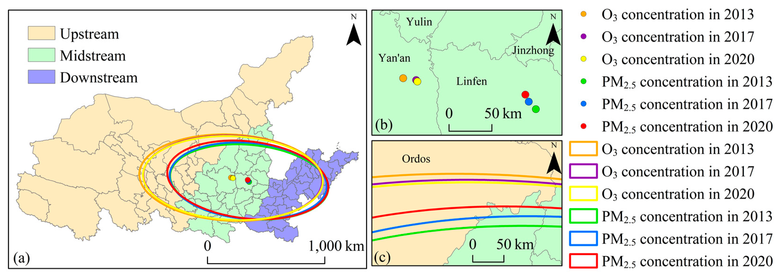
3.1.3. Centers of Gravity and SDE

Due to the shape of the YRB, flowing from west to east, combined with the distribution of air pollutant concentrations, where the high-concentration regions are mainly clustered in the downstream, the SDE for both showed a northwesterly–southeasterly direction, and the SDE of each parameter remained essentially the same, with a small change in the YRB during 2013–2020 (Table 3). Specifically, the area of the SDE of PM2.5 concentration increased gradually. The semimajor axis decreased and then increased, while the semiminor axis continued to increase. The overall change dimension of the axis was essentially the same. The rotation also presented a tendency of decreasing and then increasing. This indicated that PM2.5 concentration agglomeration in the YRB decreased slightly, while that in its northwestern and southeastern parts decreased gradually, pushing the SDE to rotate clockwise. The area of the SDE of O3 concentration decreased gradually. The semimajor axis decreased and then increased, while the semiminor axis decreased continuously, and the rotation remained stable. This indicated that O3 concentration agglomeration in the YRB increased during 2013–2020. The cities with high O3 concentrations gradually gathered in the mid-downstream regions. The center of gravity of PM2.5 concentration migrated 11.91 km to the northwest during 2013–2017 and then migrated a further 9.24 km to the northwest during 2017–2020. This indicated that PM2.5 concentration decreased in the mid-downstream regions. The center of gravity of O3 concentration migrated 15.61 km to the southeast during 2013–2017 and then continued to migrate slightly to the southeast (by 2.33 km) during 2017–2020. This indicated that the O3 concentration in the mid-downstream regions tended to aggregate. The center of gravity of PM2.5 concentration was distributed to the northwest of that of O3 concentration. Starting from 2013, the centers of gravity of the two pollutants’ concentrations continuously migrated to the northwest and southeast, respectively. The distance between their centers of gravity reduced by 30.03 km (nearly 19.05%), with a distance of only 127.61 km in 2020. This indicates that PM2.5 concentration gradually decreased and O3 concentration increased in mid-downstream regions of the YRB. (See Figure 4).

3.2. Synergistic Characteristics of the Spatial Correlation between PM2.5 and O3 Concentrations

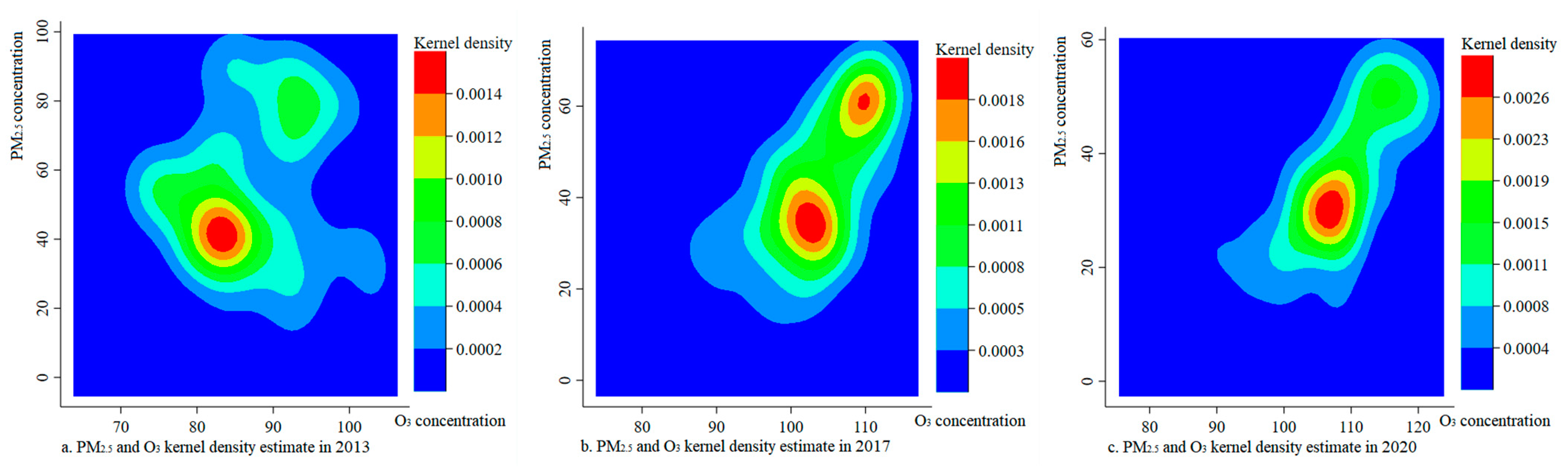
3.2.1. Synergistic Evolution Characteristic

So as to study the synergistic evolution of PM2.5 and O3 concentrations in the YRB, we plotted bivariate kernel density (Figure 5). The peak of bivariate kernel density was reached at a PM2.5 concentration of 40 μg/m3 and a O3 concentration of 85 μg/m3 in 2013, while the profile showed a sub-peak at a PM2.5 concentration of 80 μg/m3 and a O3 concentration of 95 μg/m3. The bivariate kernel densities showed a barycentric pattern in 2017, and a dual-center trend was gradually presented. The two peaks were observed when the PM2.5 concentration was 35 μg/m3 and the O3 concentration was 105 μg/m3, and when the PM2.5 concentration was 60 μg/m3 and the O3 concentration was 110 μg/m3, respectively. Compared to 2013, PM2.5 concentration at both peaks decreased, while O3 concentration increased significantly, indicating an alleviation of PM2.5 pollution and an exacerbation of O3 pollution. However, the dual-center model was changed to a single center in 2020. Only the peak at a PM2.5 concentration of 35 μg/m3 and a O3 concentration of 105 μg/m3 was retained, while the kernel density value increased. The synergistic evolution pattern in the YRB during 2013–2020 was decreasing PM2.5 concentration and increasing O3 concentration. The shift in the peak of the bivariate kernel density showed a decrease in PM2.5 concentration and an increase in O3 concentration during 2013–2020.
Figure 6 demonstrates that the trend of decreasing PM2.5 concentration and increasing O3 concentration was observed in most of the cities during 2013–2017, while a decrease in PM2.5 and O3 concentrations appeared only in the Tibetan Autonomous Prefectures of Hainan and Haibei. The PM2.5 and O3 concentrations increased in Xilingol League. Meanwhile, there was no city where PM2.5 concentration increased and O3 concentration decreased. Most cities still showed a pattern of decreasing PM2.5 and increasing O3 concentration during 2017–2020, with only Hohhot and Ulanqab showing decreases in both PM2.5 and O3 concentrations. PM2.5 and O3 concentrations increased in Alashan League, Jiuquan, and Bayannur. In Jiayuguan, PM2.5 concentration increased while O3 concentration decreased during 2017–2020.

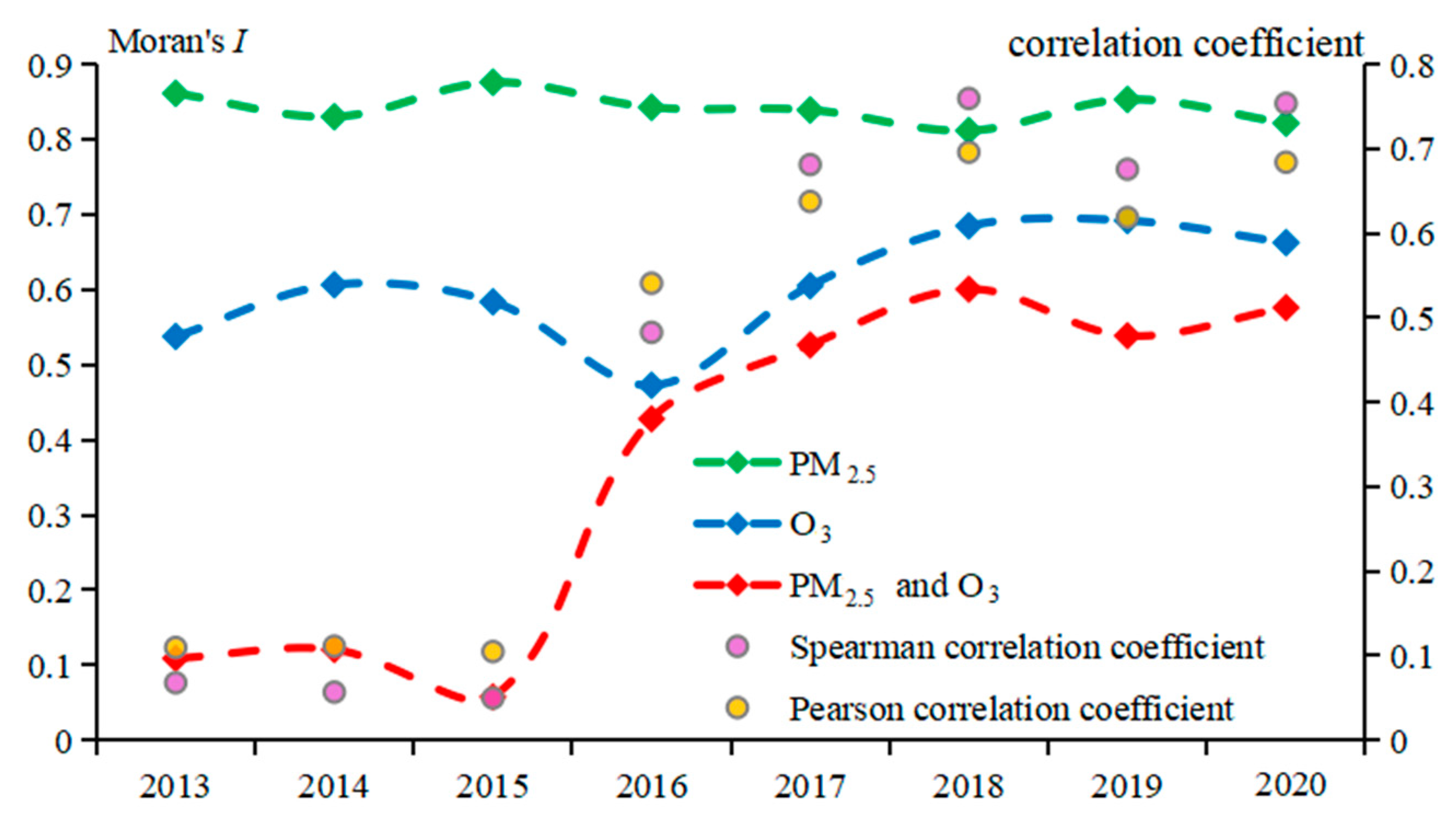
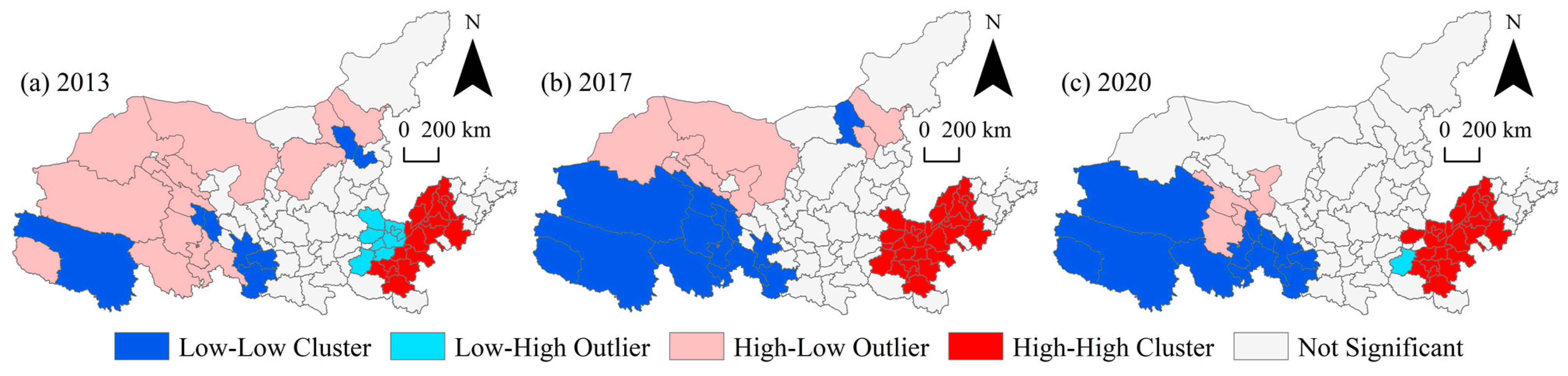
3.2.2. Spatial Auto-Correlation Characteristic

We calculated the correlation coefficients of the two pollutants’ concentrations during 2013–2020 using Stata17 (Figure 7). The correlation coefficients were at a low level and did not pass the 5% significance test during 2013–2015, while they increased dramatically to 0.541 and 0.483 in 2016, respectively. Since the Action Plan for Prevention and Control of Air Pollution, PM2.5 has been the primary target of environmental regulations, and its emissions are decreasing very quickly [48]. The emission of NOx and VOCs, the precursors of O3, is still high [3]. It is very difficult to adjust the YRB’s industrial structure in a short time [4]. Therefore, during the initial period of the policy, the correlation between PM2.5 and O3 concentrations was weak in the YRB. Meanwhile, the Chinese Ambient Air Quality Standard (GB3095-2012) was implemented in 2016, proposing further limits for the concentrations and further strengthening environmental regulations, and the trend of co-frequency changes between PM2.5 concentration and O3 concentration in neighboring regions began to appear [3]. Therefore, the correlation between the two pollutants’ concentrations began to gradually increase significantly. Both correlation coefficients reflected a fluctuating upward trend during 2017–2020. This indicates that the correlation was already strong and significant. So as to investigate the spatial auto-correlation, we measured the univariate and bivariate Moran’s I of the two pollutants’ concentrations by Geoda1.22 (Figure 7). The univariate Moran’s I of PM2.5 concentration fluctuated in the range of 0.812–0.876 during 2013–2020, indicating that PM2.5 concentration has a positive auto-correlation—that is, cities with similar PM2.5 concentrations are adjacent to one another. The univariate Moran’s I of O3 concentration fluctuated during 2013–2016, dropping to 0.473, indicating that the degree of positive spatial auto-correlation gradually weakened and the range of O3 concentration dispersed. Subsequently, the positive spatial auto-correlation degree of O3 concentration increased, while Moran’s I gradually rose to 0.663 in 2020. However, the bivariate Moran’s I was relatively low during 2013–2015, the spatial clustering features were not obvious, and the spatial correlation was weak. In 2016, the bivariate Moran’s I began to rise sharply. This indicates that spatial auto-correlation of the two pollutants’ concentrations is increasing in the YRB, showing a trend of synchronous change, and it also shows a change characteristic from dispersion to aggregation [5].
We plotted a bivariate LISA clustering map of the two pollutants’ concentrations in the YRB using Geoda1.22 (Figure 8). A total of 17 cities with high–high clustering of the two pollutants accounted for 18.89% of the cities in the YRB in 2013, most of which were distributed in its downstream. The distribution of low–low clusters was relatively decentralized, with four small-scale clusters identified: Hohhot–Shuozhou, Xining–Haidong, Dingxi–Tianshui–Longnan, and Yushu Tibetan Autonomous Prefecture. The cities with high O3 concentrations and low PM2.5 concentrations were distributed in the upstream region, accounting for 13.33% of the cities in the YRB. The eight cities with high PM2.5 concentrations and low O3 concentrations were located in Henan and Shanxi. The spatial auto-correlation of the two pollutants’ concentrations changed in 2017. The low–low cluster areas increased to 12 cities and showed a centralized distribution in the upstream region, mainly including Qinghai Province, Longnan, Tianshui, and Baotou. The high–high cluster areas also gradually expanded, accounting for 30.00%. The original region with a high PM2.5 concentration and a low O3 concentration was transformed into a high–high cluster of the two pollutants. Thus, there were no cities with high PM2.5 concentrations and low O3 concentrations in 2017. The number of agglomerating cities with high O3 concentrations and low PM2.5 concentrations decreased to six, showing two small-scale agglomerations, namely, Zhangye–Wuwei–Jiuquan–Alashan League, and Hohhot–Ulanqab. The spatial auto-correlation of the two pollutants’ concentrations changed again in 2020. The areas of low–low clustering changed; Xining, Baotou, and the Tibetan Autonomous Prefectures of Hainan and Haibei exited the low–low cluster areas, while Linxia and Tianshui entered the low–low cluster areas. The areas with high O3 concentrations and low PM2.5 concentrations further decreased, leaving only Wuwei, Xining, and the Tibetan Autonomous Prefectures of Hainan and Haibei. There was only one city (Luoyang) with a high PM2.5 concentration and a low O3 concentration in 2020. Only 23 cities remained in the high–high cluster area in 2020.
From 2013 to 2020, the clusters with low PM2.5 concentrations and high O3 concentrations in the upstream gradually decreased and were transformed into cluster areas with low PM2.5 and low O3 concentrations, mainly because the PM2.5 concentration was relatively low and continued to decline in the upstream region, while the O3 concentration increased, but its amplitude was weaker than that in the midstream and downstream region. Therefore, the upstream region formed a cluster with a low PM2.5 concentration and a low O3 concentration. The cluster with a high PM2.5 concentration and a low O3 concentration in the downstream region of the YRB was transformed into a cluster with a high PM2.5 concentration and a high O3 concentration. Although the PM2.5 concentration has decreased, it is still higher than that in up-midstream regions, and the O3 concentration in the downstream is also higher than that in other regions. The LISA cluster map further identifies the synergistic evolution pattern of decreasing PM2.5 concentration and increasing O3 concentration.

4. Discussion

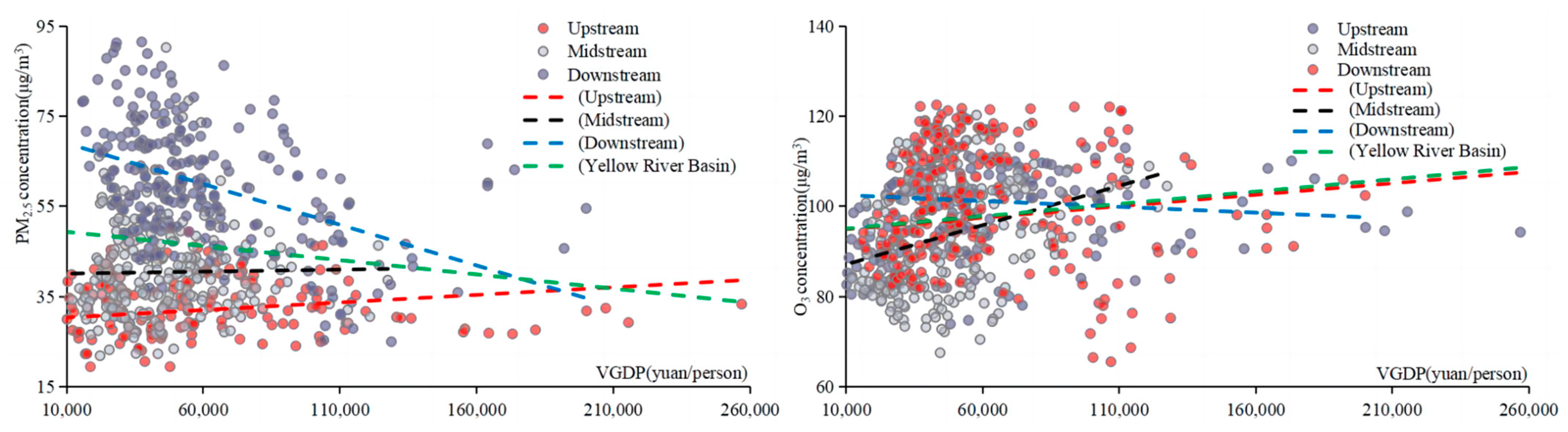
4.1. Factor Analysis of Air Pollutant Concentrations

We analyzed various factors with the EKC model to explore the synergistic changes in PM2.5 and O3 concentrations. We selected PM2.5 and O3 concentrations as dependent variables, and we took per capita GDP and its square and cubic terms as the core explanatory variables. So as to ensure the validity of the regression and avoid the phenomenon of pseudo-regression, descriptive statistics and HT stationarity tests were conducted for each variable (Table 4).
So as to further visualize the effect of the regional economy on air pollution, scatter-fit plots of the two pollutants’ concentrations and per capita GDP in the YRB and its upstream, midstream, and downstream regions were plotted separately (Figure 9). According to the scatter-fit plots, there is a more obvious correlation between the two pollutants’ concentrations and per capita GDP. Furthermore, based on the EKC, we constructed a panel regression model to analyze factors for PM2.5 and O3 concentrations during 2013–2020. We constructed fixed-effects (FE) models and random-effects (RE) models (Table 5). Combining the regression of the Hausman test and models’ R2, as well as the significance test of each variable, the FE models are more appropriate for explaining the factors.
Model II demonstrates that the effects of per capita GDP and its square and cubic terms on PM2.5 concentration passed significance test. This indicates that there is an obvious relationship between economy and PM2.5 concentration. However, it does not conform to the classic inverted “U-shaped” EKC, but rather to the “N-shape”. This is consistent with the findings of Wang and Komonpipat [60], showing a significant three-stage correlation. PM2.5 concentration will increase by 21.28% if per capita GDP increases by 1% when per capita GDP is less than 15,242 RMB. Meanwhile, when it ranges from 15,242 to 156,315 RMB, PM2.5 concentration will decrease by 1.989% if per capita GDP increases by 1%, and when it exceeds 156,315 RMB, PM2.5 concentration will increase again by 0.06% if per capita GDP increases by 1%.
O3 concentration showed an opposite result compared with the PM2.5 concentration. Model IV demonstrates that the effects of per capita GDP and its square and cubic terms on O3 concentration also passed the significance test, presenting an obvious inverted “N-shaped” curve between economy and O3 concentration. This is consistent with the shape of the EKC between O3 concentration and per capita GDP in China, but with differences in the location of its inflection point [56]. The first inflection point in the YRB is later than that in China (14,811 RMB), but the second inflection point is earlier than that in China (410,674 RMB). When per capita GDP is less than 18,118 RMB, O3 concentration will decrease by 31.87% if per capita GDP increases by 1% in the YRB. When it ranges from 18,118 RMB to 141,712 RMB, O3 concentration will increase by 2.96% if per capita GDP increases by 1%, and when it exceeds 141,712 RMB, O3 concentration will decrease again by 0.09% if per capita GDP increases by 1%.
Urbanization has an important impact on air pollution [17]. Model II and Model IV demonstrate that PM2.5 concentration will decrease by 0.53% if PU increases by 1%, while O3 concentration will increase by 0.36%. PD passed the significance test only in Model IV. O3 concentration will increase by 0.10% if PD increases by 1%. The industrial upgrading has a vital significance to reduce air pollution [39]. The effects of the Ind on PM2.5 and O3 concentrations passed the significance test, while the directions differed, showing an inhibitory effect on PM2.5 concentration and a promotional effect on O3 concentration. At present, industrial upgrading has significantly reduced PM2.5 concentration, but it has not reduced O3 concentration, mainly because of the high dependence on natural resources and the industrial structure of coal, steel, and other resource-intensive industries [46]. The need for large-scale capital investment is mainly because most cities have a heavy industrial structure, and the heavy chemical industry chain is a capital-intensive industry [48]. Meanwhile, VOCs and NOx emissions are still at high levels, and it is difficult for the industry to achieve sophistication and green transformation in the YRB in the short term. With regard to natural factors, the NDVI presents a promotional effect on air pollutants, while its effect on O3 concentration did not pass the significance test. The annual average precipitation shows an inhibitory effect on air pollutants, but only its effect on O3 concentration passed the significance test. O3 concentration will decrease by 0.13% if the annual average precipitation increases by 1%. In terms of air mobility, PM2.5 concentration will decrease by 0.11% if ventilation coefficients increase by 1%, while O3 concentration will increase by 0.07%.

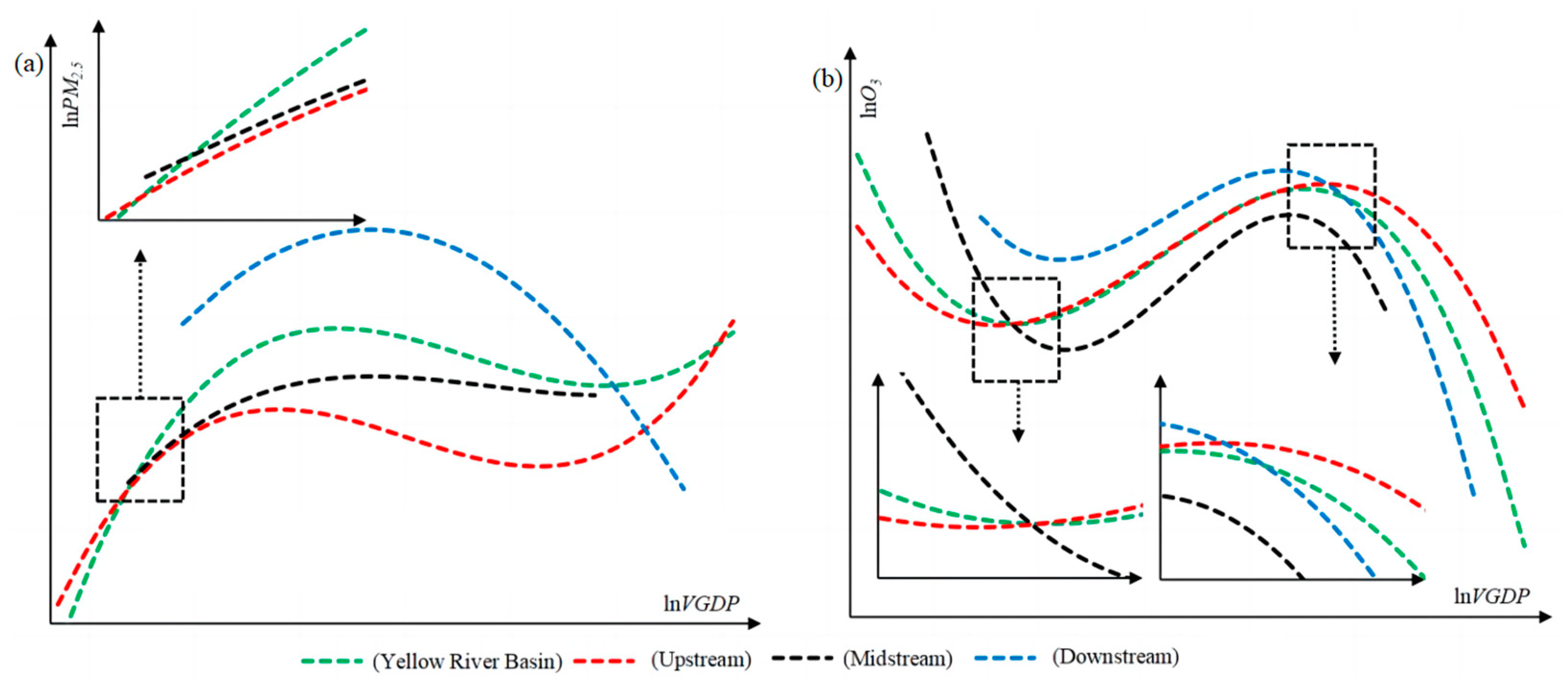
4.2. Heterogeneity Analysis from Different Sub-Watersheds

In order to better explore the heterogeneity of factors from different sub-watersheds for the two pollutants’ concentrations in the YRB, we constructed FE models (Models V–X). The influence direction and intensity of the effects showed obvious heterogeneity in the different sub-watersheds (Table 6).
The correlation between economy and PM2.5 concentration shows a significant three-stage “N-shaped” curve in the upstream region (Figure 10a). When per capita GDP is lower than 8685 RMB, if per capita GDP increases by 1%, the PM2.5 concentration will increase by 13.55%, and when it ranges from 8685 RMB to 13,813 RMB, PM2.5 concentration will decrease by 1.32% if per capita GDP increases by 1%. When per capita GDP exceeds 131,813 RMB, the PM2.5 concentration will increase again by 0.04% if per capita GDP increases by 1%. The sensitivity of the effect of per capita GDP on PM2.5 concentration in the upstream is weaker than that in the overall YRB. The upstream air pollution base is better than those of the mid-downstream, and the economic growth is relatively slow, so the effect of per capita GDP on air pollution is relatively weak [48]. The correlation between economy and PM2.5 concentration in the midstream region also shows a three-stage “N-shaped” curve. When per capita GDP in the midstream region is lower than 17,969 RMB, if per capita GDP increases by 1%, the PM2.5 concentration will increase by 37.02%. Meanwhile, when it ranges from 17,969 RMB to 102,881 RMB, if per capita GDP increases by 1%, PM2.5 concentration will decrease by 3.49%. When per capita GDP is more than 102,881 RMB, PM2.5 concentration will increase again by 0.11% if per capita GDP increases by 1%. The sensitivity of the effect of per capita GDP on PM2.5 concentration in the midstream is stronger than that in the upstream and the overall YRB. The correlation between economy and PM2.5 concentration is in accordance with the EKC theory, showing an inverted “U-shape”. If per capita GDP increases by 1%, the PM2.5 concentration will increase by 1.70% when per capita GDP is lower than 27,662 RMB in the downstream region. When per capita GDP exceeds 27,662 RMB, PM2.5 concentration will decrease by 0.08% if per capita GDP increases by 1% in the downstream region. Existing studies have explored the impact of digital economy on PM2.5 concentration. There are more high-pollution enterprises, and the ecological environment governance pressure is greater, and PM2.5 concentration is declining more rapidly in the midstream region. The higher population urbanization and the stronger economic development in the downstream region can also better improve air pollution [40], which is broadly consistent with our results.
Models VIII–X demonstrate the regression models that affect O3 concentration in the different sub-watersheds. The correlations between economy and PM2.5 concentration all show an inverted “N shaped” in the upstream, midstream, and downstream regions (Figure 10b). However, there is significant sensitivity of the differentiated effect of per capita GDP on O3 concentration. When per capita GDP is lower than 12,635 RMB in the upstream region, O3 concentration will decrease by 23.61% if per capita GDP increases by 1%. When per capita GDP ranges from 12,635 RMB to 133,944 RMB, O3 concentration will increase by 2.25% if per capita GDP increases by 1%, and when per capita GDP exceeds 133,944 RMB, O3 concentration will decrease by 0.07% if per capita GDP increases by 1%. In the midstream region, when per capita GDP is lower than 20,024 RMB, O3 concentration will decrease by 69.04% if per capita GDP increases by 1%. Meanwhile, when it ranges from 20,024 RMB to 109,887 RMB, O3 concentration will increase by 6.46% if per capita GDP increases by 1%. When per capita GDP exceeds 109,887 RMB, O3 concentration will decrease by 0.20% if per capita GDP increases by 1%. In the downstream region, when per capita GDP is lower than 31,059 RMB, O3 concentration will decrease by 17.68% if per capita GDP increases by 1%. When per capita GDP ranges from 31,059 RMB to 141,572 RMB, O3 concentration will increase by 1.59% if per capita GDP increases by 1%. Meanwhile, when per capita GDP exceeds 141,572 RMB, O3 concentration will decrease again by 0.05% if per capita GDP increases by 1%. Therefore, the sensitivity of the effect of per capita GDP on O3 concentration is the strongest in the midstream region. In the upstream region, the economic development level is weak and the air pollution concentrations are low, while air pollution concentrations are high and the economic development level is also high in the downstream region [46]. However, the midstream region is rich in energy, with a complete heavy chemical industry system, and located in the Loess Plateau, where the economic development mode is extensive and slow but air pollution is serious, and the conflict between humans and land is the most severe [61]. Therefore, the sensitivity of the effect of per capita GDP on O3 concentration is the strongest in the midstream region.
Combined with the EKC between economy and air pollution (Figure 11), a critical transition period for environmental quality improvement appears in the YRB [50]. The inflection point at which PM2.5 concentration begins to decrease with per capita GDP in the YRB is 15,242 RMB, while there are different and specific inflection points in various sub-watersheds. The inflection point in the downstream region (27,662 RMB) is higher than that in the midstream (17,969 RMB) and upstream (8685 RMB) regions. The highest inflection point of per capita GDP occurred in the downstream region (27,662 RMB), mainly because, in the early stages, in exchange for rapid economic development, large amounts of air pollutants were discharged [62], resulting in a relatively slow process of air pollution mitigation. However, we need to be alert to the risk of PM2.5 concentration rising again in the YRB. There is a risk of elevated air pollution emissions with the slowing down of economic growth rate, and a risk in the up-midstream regions undertaking the transfer of polluting industries from the downstream region [46]. The EKC indicates that PM2.5 concentration has gradually decreased, although there is still a certain distance from the lifting inflection point. It is necessary to prevent this pollutant’s concentration from rising again [47]. The inflection point of O3 concentration changing from decreasing to increasing with per capita GDP is 18,118 RMB in the YRB. Therefore, the inflection point of increasing O3 concentration (18,118 RMB) is higher than that of decreasing PM2.5 concentration (15,242 RMB), indicating that the mitigation of O3 pollution takes place later than that of PM2.5 pollution (Figure 11). Existing studies have also concluded that as PM2.5 concentration increases, O3 concentration also decreases, and the decrease in PM2.5 takes place earlier than for O3 concentration [15]. However, there are some differences in the specific inflection points in different sub-watersheds. The main thing to note is that the inflection point of O3 concentration increase in the downstream region (31,059 RMB) is still higher than that in the midstream and upstream regions (20,024 RMB and 12,635 RMB, respectively), which is consistent with the overall spatial pattern. Currently, O3 concentration is still in a state of pollution deterioration in the YRB, which is also a vital factor restricting the sustainable development of the YRB [47]. According to the EKC, the inflection point where O3 concentration changes from increasing to decreasing with per capita GDP is 141,712 RMB in the YRB, which is lower than the inflection point at which PM2.5 concentration changes from decreasing to increasing in the YRB (156,315 RMB). Currently, there still exists a large gap between economy and better air quality in the YRB, so it is expected that O3 concentration will decrease first and PM2.5 concentration will increase [63]. The inflection point of O3 concentration reduction is 141,572 RMB in the downstream region, which is higher than that in the up-midstream regions (133,944 RMB and 109,887 RMB, respectively). However, if O3 concentration is to be reduced across the board, great efforts will need to be made in all sub-watersheds. In particular, economy is relatively weak in the upstream region, for the sake of achieving coordinated progress in ecological improvement and sustainable development; only the implementation of integrated and coordinated air pollution control [48] can better promote high-quality development in various sub-watersheds.
Climate change and air pollution threaten human health and security [64]. The synergy of PM2.5 and O3 governance, the synergy of air quality and health effects, and the synergy of atmospheric environment and climate will be the main trends of atmospheric environment governance [2]. The synergistic evolution pattern of decreasing PM2.5 concentration and increasing O3 concentration in the YRB indicates that pollutant discharge is still high. Meanwhile, air pollution and climate change have homologous characteristics, and both produce different degrees of health impacts in different ways [65]. Existing studies indicate that implementing a collaborative path to low carbon and clean air could prevent at least 2 million premature deaths caused by air pollution each year [66]. Despite being subject to strong environmental regulations, the formation of O3 is partially offset by significant reductions in NOx and VOCs. However, six of the warmest years on record took place during 2013–2020, and rising temperatures will aggravate the increase in O3 concentration, which poses a serious threat to human survival [7,8]. At present, the industry in the YRB is in an important period of transition, but carbon emissions and air pollution emissions are still at high levels [48]. Therefore, adjusting the industrial structure, energy structure, transportation, and other comprehensive measures is essential to strengthen the decrease in NOx and VOCs concentrations [5]. In the process of adjusting the industrial structure and energy structure, the consumption of fossil energy has decreased, the consumption of non-fossil clean energy has increased significantly [30]. The emissions of CO2 and air pollutants will undergo fundamental changes, and the changes in energy layout, industrial layout, and emissions will further have a positive effect on the ecological environment [67]. Special management for different air pollutants not only should to be implemented, but also should to reduce production of their pollutant precursors, minimize the internal transformation of pollutants, and avoid the situation where O3 concentration will continue to rise while PM2.5 concentration will decrease significantly [26]. Hence, it is meaningful to follow the general direction of carbon and pollution reduction in the YRB [50]. In the process of achieving carbon neutrality and continuously improving air quality, health drives the common management of air and climate change [47]. It is crucial to improve the joint management mechanism for air pollution, effectively coordinating the strategies of health protection and clean air, safe climate, sustainable energy, and economic development, and achieving the harmony of man and nature in large river basins [68].

5. Conclusions and Prospects

5.1. Main Conclusions

So as to recognize the synergistic evolution of PM2.5 and O3 concentrations and help formulate relevant policies for their synergistic control, we investigated the spatiotemporal synergistic evolution and factors related to them in the YRB during 2013–2020. Our specific findings are that PM2.5 concentration presented a fluctuating downward in the YRB and its sub-watersheds, with the largest decrease in its downstream region. O3 concentration presented a sharp increase in the YRB, with the largest increase in its midstream region. The spatial evolution of the centers of gravity and SDE reflected that the cities showed a gradual decrease in PM2.5 concentration and an increase in O3 concentration. With the help of bivariate kernel density, we found that the synergistic evolution of PM2.5 and O3 concentrations was characterized by a decrease in PM2.5 concentration and an increase in O3 concentration during 2013–2020, with only several cities in the north showing a differentiated evolution trend. A strong positive spatial correlation was observed between the two pollutants, among which the low–low cluster was mostly located in Qinghai and Gansu, the high–high cluster was located in Henan and Shandong. PM2.5 concentration showed an “N-shaped” correlation with economy in the YRB, whereas O3 concentration showed an inverted “N-shaped” correlation with economy. The correlations between economy and PM2.5 concentration were “N shaped”, “N shaped”, and inverted “U shaped” in the upstream, midstream, and downstream, respectively. The sensitivity of per capita GDP to PM2.5 concentration in the midstream was stronger than that in the upstream. There was an inverted “N-shaped” correlation between O3 concentration and economy in the all of sub-watersheds, and the sensitivity of per capita GDP to O3 concentration was stronger in the midstream than in the upstream and downstream. The EKCs showed that the increase in inflection point of O3 concentration was higher than the decrease in inflection point of PM2.5 concentration. It is expected that O3 concentration will decrease first and then PM2.5 concentration will increase. Combined with the inflection point and shape of the EKCs, the synergistic evolution pattern is that PM2.5 concentration gradually decreases and O3 concentration gradually increases in the YRB.

5.2. Research Limitations and Future Research Prospects

The innovation lies in analyzing the synergistic evolution of PM2.5 and O3 concentrations, analyzing their factors in the YRB with the help of EKCs, and analyzing the mechanism underlying the relationship between economy and air pollution. This will be useful to help scholars better understand their synergistic trend and provide corresponding references for the government to formulate relevant policies for synergistic control of air pollutants. Nevertheless, there are still many shortcomings. Firstly, only 78 of these 90 cities were selected in the YRB when constructing the econometric model, because those in the upstream region are mainly minority autonomous prefectures. We did not obtain equivalent amounts of socio-economic data in the middle and downstream regions. The EKC study ignored the dynamic bidirectional relationship between economy and environment and analyzed only the effect of economy on air pollution, which might have an impact on the accuracy of the model’s estimations. Secondly, EKCs’ ability to interpret reality is seriously affected by the industrial transfer, whereby not all pollutants disappear, but part of pollution is transferred to other regions. The up-midstream regions of the YRB, as the main relocation sites of the downstream polluting industries, have suffered such pollution transfer. From the perspective of all large basins, air pollution may not be reduced but transferred, so the explanatory ability of EKC models may be insufficient. In a follow-up study, we could start from the industrial transfer from downstream to up-midstream regions to explore its impact. The Yangtze River Economic Belt (YREB) has long been vital supports for China’s development. The development model in the YREB is ahead of that in the YRB. The mechanism underlying the correlation between economy and environment pollution in the YRB and the YREB could be studied comparatively in future studies, with the aim of facilitating the early arrival of the inflection point of air pollution in the YRB by analyzing the patterns of regions with higher-quality economy, such as the YREB. CO2 and air pollution have the same root, homology and interaction correlation attributes. We can concentrate on the synergistic effect of CO2–PM2.5–O3 under the path of “carbon peak” in subsequent studies.

Author Contributions

Conceptualization, C.W.; data curation, G.Q. and C.T.; funding acquisition, C.W.; methodology, G.Q.; supervision, Z.W.; writing—original draft, G.Q., Y.M. and F.X.; writing—review and editing, Z.W. All authors have read and agreed to the published version of the manuscript.

Funding

This word is funded by National Natural Science Foundation of China, Grant Number 42201182, also funded by the Major Project of Key Research Bases for Humanities and Social Sciences Funded by the Ministry of Education of China, Grant Number 22JJD790015.

Institutional Review Board Statement

Not applicable.

Informed Consent Statement

Not applicable.

Data Availability Statement

The data presented in this study are available on request from the corresponding author.

Conflicts of Interest

The authors declare no conflict of interest.

References

  1. Wu, H.; Guo, B.; Guo, T.; Pei, L.; Jing, P.; Wang, Y.; Ma, X.; Bai, H.; Wang, Z.; Xie, T.; et al. A study on identifying synergistic prevention and control regions for PM2.5 and O3 and exploring their spatiotemporal dynamic in China. Environ. Pollut. 2024, 341, 122880. [Google Scholar] [CrossRef] [PubMed]
  2. Xiao, Q.; Geng, G.; Xue, T.; Liu, S.; Cai, C.; He, K.; Zhang, Q. Tracking PM2.5 and O3 Pollution and the Related Health Burden in China 2013–2020. Environ. Sci. Technol. 2022, 56, 6922–6932. [Google Scholar] [CrossRef] [PubMed]
  3. Ma, M.; Liu, M.; Song, X.; Liu, M.; Fan, W.; Wang, Y.; Xing, H.; Meng, F.; Lv, Y. Spatiotemporal patterns and quantitative analysis of influencing factors of PM2.5 and O3 pollution in the North China Plain. Atmos. Pollut. Res. 2024, 15, 101950. [Google Scholar] [CrossRef]
  4. Du, S.; He, C.; Zhang, L.; Zhao, Y.; Chu, L.; Ni, J. Policy implications for synergistic management of PM2.5 and O3 pollution from a pattern-process-sustainability perspective in China. Sci. Total Environ. 2024, 915, 170210. [Google Scholar] [CrossRef] [PubMed]
  5. Shao, T.; Wang, P.; Yu, W.; Gao, Y.; Zhu, S.; Zhang, Y.; Hu, D.; Zhang, B.; Zhang, H. Drivers of alleviated PM2.5 and O3 concentrations in China from 2013 to 2020. Resour. Conserv. Recycl. 2023, 197, 107110. [Google Scholar] [CrossRef]
  6. Liu, Y.; Geng, G.; Cheng, J.; Liu, Y.; Xiao, Q.; Liu, L.; Shi, Q.; Tong, D.; He, K.; Zhang, Q. Drivers of increasing Ozone during the two phases of Clean Air Actions in China 2013–2020. Environ. Sci. Technol. 2023, 57, 8954–8964. [Google Scholar] [CrossRef] [PubMed]
  7. Cheng, C.; Liu, Y.; Han, C.; Fang, Q.; Cui, F.; Li, X. Effects of extreme temperature events on deaths and its interaction with air pollution. Sci. Total Environ. 2024, 915, 170212. [Google Scholar] [CrossRef] [PubMed]
  8. Peng, M.; Zhang, F.; RMB, Y.; Yang, Z.; Wang, K.; Wang, Y.; Tang, Z.; Zhang, Y. Long-term ozone exposure and all-cause mortality: Cohort evidence in China and global heterogeneity by region. Ecotoxicol. Environ. Saf. 2024, 270, 115843. [Google Scholar] [CrossRef] [PubMed]
  9. Demoury, C.; Aerts, R.; Berete, F.; Wouter, L.; Pauwels, A.; Vanpoucke, C.; Heyden, J.; Clercq, E. Impact of short-term exposure to air pollution on natural mortality and vulnerable populations: A multi-city case-crossover analysis in Belgium. Environ. Health 2024, 23, 11. [Google Scholar] [CrossRef]
  10. Liu, Z.; Qi, Z.; Ni, X.; Dong, M.; Ma, M.; Xue, W.; Zhang, Q.; Wang, J. How to apply O3 and PM2.5 collaborative control to practical management in China: A study based on meta-analysis and machine learning. Sci. Total Environ. 2021, 772, 145392. [Google Scholar] [CrossRef]
  11. Chen, L.; Zhu, J.; Liao, H.; Yang, Y.; Yue, X. Meteorological influences on PM2.5 and O3 trends and associated health burden since China’s clean air actions. Sci. Total Environ. 2020, 744, 140837. [Google Scholar] [CrossRef] [PubMed]
  12. Gu, Y.; Liu, B.; Meng, H.; Song, S.; Dai, Q.; Shi, L.; Feng, Y.; Hopke, P. Source apportionment of consumed volatile organic compounds in the atmosphere. J. Hazard. Mater. 2023, 459, 132138. [Google Scholar] [CrossRef] [PubMed]
  13. Liu, J.; Ma, F.; Chen, T.; Jiang, D.; Du, M.; Zhang, X.; Feng, X.; Wang, Q.; Cao, J.; Wang, J. High-time resolution PM2.5 source apportionment assisted by spectrum-based characteristics analysis. Sci. Total Environ. 2024, 912, 169055. [Google Scholar] [CrossRef] [PubMed]
  14. Wu, J.; Wang, Y.; Liang, J.; Yao, F. Exploring common factors influencing PM2.5 and O3 concentrations in the Pearl River Delta: Tradeoffs and synergies. Environ. Pollut. 2021, 285, 117138. [Google Scholar] [CrossRef] [PubMed]
  15. Qu, Y.; Wang, T.; Yuan, C.; Wu, H.; Gao, L.; Huang, C.; Li, Y.; Li, M.; Xie, M. The underlying mechanisms of PM2.5 and O3 synergistic pollution in East China: Photochemical and heterogeneous interactions. Sci. Total Environ. 2023, 873, 162434. [Google Scholar] [CrossRef] [PubMed]
  16. Gauthier-Manuel, H.; Bernard, N.; Boilleaut, M.; Giraudoux, P.; Pujo, L.; Mauny, F. Spatialized temporal dynamics of daily ozone concentrations: Identification of the main spatial differences. Environ. Int. 2023, 173, 107859. [Google Scholar] [CrossRef] [PubMed]
  17. Qi, G.; Wang, Z.; Wei, L.; Wang, Z. Multidimensional effects of urbanization on PM2.5 concentration in China. Environ. Sci. Pollut. Res. 2022, 29, 77081–77096. [Google Scholar] [CrossRef] [PubMed]
  18. Duan, W.; Wang, X.; Cheng, S.; Wang, R. Regional division and influencing mechanisms for the collaborative control of PM2.5 and O3 in China: A joint application of multiple mathematic models and data mining technologies. J. Clean. Prod. 2022, 337, 130607. [Google Scholar] [CrossRef]
  19. Saha, P.; Sengupta, S.; Adams, P.; Robinson, A.; Presto, A. Spatial Correlation of Ultrafine Particle Number and Fine Particle Mass at Urban Scales: Implications for Health Assessment. Environ. Sci. Technol. 2020, 54, 9295–9304. [Google Scholar] [CrossRef]
  20. Chen, Y.; Li, H.; Karimian, H.; Li, M.; Fan, Q.; Xu, Z. Spatio-temporal variation of ozone pollution risk and its influencing factors in China based on Geodetector and Geospatial models. Chemosphere 2022, 302, 134843. [Google Scholar] [CrossRef]
  21. Liu, J.; Wang, S.; Zhu, K.; Hu, J.; Li, R.; Song, X. Spatial patterns of the diurnal variations of PM2.5 and their influencing factors across China. Atmos. Environ. 2024, 318, 120215. [Google Scholar] [CrossRef]
  22. Zhang, Q.; Zheng, Y.; Tong, D.; Shao, M.; Wang, S.; Zhang, Y.; Xu, L.; Wang, J.; He, H.; Hao, J.; et al. Drivers of improved PM2.5 air quality in China from 2013 to 2017. Proc. Natl. Acad. Sci. 2019, 116, 24463–24469. [Google Scholar] [CrossRef] [PubMed]
  23. Tao, C.; Zhang, Q.; Huo, S.; Ren, Y.; Han, S.; Wang, Q.; Wang, W. PM2.5 pollution modulates the response of ozone formation to VOC emitted from various sources: Insights from machine learning. Sci. Total Environ. 2024, 916, 170009. [Google Scholar] [CrossRef] [PubMed]
  24. Zhang, Y.; Liu, X.; Zhang, L.; Tang, A.; Goulding, K.; Collett, J. Evolution of secondary inorganic aerosols amidst improving PM2.5 air quality in the North China plain. Environ. Pollut. 2021, 281, 117027. [Google Scholar] [CrossRef] [PubMed]
  25. Yan, D.; Jin, Z.; Zhou, Y.; Li, M.; Zhang, Z.; Wang, T.; Zhuang, B.; Li, S.; Xie, M. Anthropogenically and meteorologically modulated summertime ozone trends and their health implications since China’s clean air actions. Environ. Pollut. 2024, 343, 123234. [Google Scholar] [CrossRef] [PubMed]
  26. Liu, J.; Ding, W. Spatial and temporal distribution of PM2.5 and O3 in north China from 2011 to 2020: Patterns and influence mechanisms. Atmos. Pollut. Res. 2023, 14, 101906. [Google Scholar] [CrossRef]
  27. Meng, Z.; Dabdub, D.; Seinfeld, J. Chemical coupling between atmospheric ozone and particulate matter. Science 1997, 277, 5322. [Google Scholar] [CrossRef]
  28. Li, K.; Jacob, D.J.; Shen, L.; Lu, X.; De Smedt, I.; Liao, H. Increases in surface ozone pollution in China from 2013 to 2019: Anthropogenic and meteorological influences. Atmos. Chem. Phys. 2020, 20, 11423–11433. [Google Scholar] [CrossRef]
  29. Benchrif, A.; Wheida, A.; Tahri, M.; Mezouari, H.; Bouziane, M.; El Alami, A.A.; Tachb, K. Air quality during three COVID-19 lockdown phases: AQI, PM2.5 and NO2 assessment in cities with more than 1 million inhabitants. Sustain. Cities Soc. 2021, 5, 103170. [Google Scholar] [CrossRef]
  30. Wang, Y.; Yao, L.; Xu, Y.; Sun, S.; Li, T. Potential heterogeneity in the relationship between urbanization and air pollution, from the perspective of urban agglomeration. J. Clean. Prod. 2021, 298, 126822. [Google Scholar] [CrossRef]
  31. Wu, W.; Zhang, M.; Ding, Y. Exploring the effect of economic and environment factors on PM2.5 concentration: A case study of the Beijing-Tianjin-Hebei region. J. Environ. Manag. 2020, 268, 110703. [Google Scholar] [CrossRef]
  32. Qi, G.; Wei, W.; Wang, Z.; Wang, Z.; Wei, L. The spatial-temporal evolution mechanism of PM2.5 concentration based on China’s climate zoning. J. Environ. Manag. 2023, 325, 116671. [Google Scholar] [CrossRef] [PubMed]
  33. Yang, K.; Teng, M.; Luo, Y.; Zhou, X.; Zhang, M.; Sun, W.; Li, Q. Human activities and the natural environment have induced changes in the PM2.5 concentrations in Yunnan Province, China, over the past 19 years. Environ. Pollut. 2020, 265, 114878. [Google Scholar] [CrossRef] [PubMed]
  34. Krall, J.R.; Mulholland, J.A.; Russell, A.G.; Balachandran, S.; Winquist, A.; Tolbert, P.E.; Waller, L.A.; Sarnat, S.E. Associations between source-specific fine particulate matter and emergency department visits for respiratory disease in four U.S. cities. Environ. Health Perspect. 2017, 125, 97–103. [Google Scholar] [CrossRef] [PubMed]
  35. Dadashazar, H.; Ma, L.; Sorooshian, A. Sources of pollution and interrelationships between aerosol and precipitation chemistry at a central California site. Sci. Total Environ. 2019, 651, 1776–1787. [Google Scholar] [CrossRef] [PubMed]
  36. Prottay, M.; Sadib, B.; Jobaer, A.; Rafizul, I.; Asif, I. Measuring and modeling PM2.5 zonal distributions, assembling geospatial and meteorological variables in the Khulna metropolitan area. Urban Clim. 2023, 49, 101518. [Google Scholar] [CrossRef]
  37. Zha, H.; Wang, R.; Feng, X.; An, C.; Qian, J. Spatial characteristics of the PM2.5/PM10 ratio and its indicative significance regarding air pollution in Hebei Province, China. Environ. Monit. Assess. 2021, 193, 486. [Google Scholar] [CrossRef] [PubMed]
  38. Liu, H.; Cui, W.; Zhang, M. Exploring the causal relationship between urbanization and air pollution: Evidence from China. Sustain. Cities Soc. 2022, 80, 103783. [Google Scholar] [CrossRef]
  39. Qi, G.; Wang, Z.; Wang, Z.; Wei, L. Has industrial upgrading improved air pollution?—Evidence from China’s digital economy. Sustainability 2022, 14, 8967. [Google Scholar] [CrossRef]
  40. Zhao, H.; Cheng, Y.; Zheng, R. Impact of the digital economy on PM2.5: Experience from the middle and lower reaches of the Yellow River Basin. Int. J. Environ. Res. Public Health 2022, 19, 17094. [Google Scholar] [CrossRef]
  41. Tang, Y.; Xie, S.; Huang, L.; Liu, L.; Wei, P.; Zhang, Y.; Meng, C. Spatial estimation of regional PM2.5 concentrations with GWR models using PCA and RBF interpolation optimization. Remote Sens. 2022, 14, 5626. [Google Scholar] [CrossRef]
  42. Wang, S.; Ren, Y.; Xia, B. PM2.5 and O3 concentration estimation based on interpretable machine learning. Atmos. Pollut. Res. 2023, 14, 101866. [Google Scholar] [CrossRef]
  43. Zhou, L.; Wu, T.; Pu, L.; Meadows, M.; Jiang, G.; Zhang, J.; Xie, X. Spatially heterogeneous relationships of PM2.5 concentrations with natural and land use factors in the Niger River Watershed, West Africa. J. Clean. Prod. 2023, 394, 136406. [Google Scholar] [CrossRef]
  44. Tang, Y.; Zhang, X.; Lu, S.; Taghizadeh-Hesary, F. Digital finance and air pollution in China: Evolution characteristics, impact mechanism and regional differences. Resour. Policy 2023, 86, 104073. [Google Scholar] [CrossRef]
  45. Liu, Y.; Yuan, L. Study on the influencing factors and profitability of horizontal ecological compensation mechanism in Yellow River Basin of China. Environ. Sci. Pollut. Res. 2023, 30, 87353–87367. [Google Scholar] [CrossRef] [PubMed]
  46. Zhao, H.; Liu, Y.; Gu, T.; Zheng, H.; Wang, Z.; Yang, D. Identifying spatiotemporal heterogeneity of PM2.5 concentrations and the key influencing factors in the middle and lower reaches of the Yellow River. Remote Sens. 2022, 14, 2643. [Google Scholar] [CrossRef]
  47. Wang, X.; Zhang, Q.; Chang, W.-Y. Does economic agglomeration affect haze pollution? Evidence from China’s Yellow River basin. J. Clean. Prod. 2022, 335, 130271. [Google Scholar] [CrossRef]
  48. Liu, Y.; Cheng, Y.; Zheng, R.; Zhao, H.; Wang, Y. Impact of the producer services agglomeration on PM2.5: A case study of the Yellow River Basin, China. J. Geogr. Sci. 2023, 33, 2295–2320. [Google Scholar] [CrossRef]
  49. Zhang, Q.; Zhang, Z.; Shi, P.; Singh, V.; Gu, X. Evaluation of ecological instream flow considering hydrological alterations in the Yellow River Basin, China. Glob. Planet. Change 2018, 160, 61–74. [Google Scholar] [CrossRef]
  50. Yuan, X.; Sheng, X.; Chen, L.; Tang, Y.; Li, Y.; Jia, Y.; Qu, D.; Wang, Q.; Ma, Q.; Zuo, J. Carbon footprint and embodied carbon transfer at the provincial level of the Yellow River Basin. Sci. Total Environ. 2022, 803, 149993. [Google Scholar] [CrossRef]
  51. Wang, D.; Liu, Y.; Cheng, Y. Effects and spatial spillover of manufacturing agglomeration on carbon emissions in the Yellow River Basin, China. Sustainability 2023, 15, 9386. [Google Scholar] [CrossRef]
  52. Zhang, S.; Lv, Y.; Zhang, B. Spatio-temporal evolution and influencing factors of green development in the Yellow River Basin of China. Sustainability 2022, 14, 12407. [Google Scholar] [CrossRef]
  53. Chen, Y.; Liu, S.; Ma, W.; Zhou, Q. Assessment of the carrying capacity and suitability of spatial resources and the environment and diagnosis of obstacle factors in the Yellow River Basin. Int. J. Environ. Res. Public Health 2023, 20, 3496. [Google Scholar] [CrossRef]
  54. Lefever, D. Measuring geographic concentration by means of the standard deviational ellipse. Am. J. Sociol. 1926, 1, 88–94. [Google Scholar] [CrossRef]
  55. Emanuel, P. On estimation of a probability density function and mode. Ann. Math. Stat. 1962, 33, 1065–1076. [Google Scholar] [CrossRef]
  56. Qi, G.; Che, J.; Wang, Z. Differential effects of urbanization on air pollution: Evidences from six air pollutants in mainland China. Ecol. Indic. 2023, 146, 109924. [Google Scholar] [CrossRef]
  57. Anselin, L. Local indicators of spatial association: LISA. Geogr. Anal. 1995, 27, 93–115. [Google Scholar] [CrossRef]
  58. Grossman, G.; Krueger, A. Economic growth and the environment. Q. J. Econ. 1995, 110, 353–377. [Google Scholar] [CrossRef]
  59. Hering, L.; Poncet, S. Environmental policy and exports: Evidence from Chinese cities. J. Environ. Econ. Manag. 2014, 68, 296–318. [Google Scholar] [CrossRef]
  60. Wang, Y.; Komonpipat, S. Revisiting the environmental Kuznets curve of PM2.5 concentration: Evidence from prefecture-level and above cities of China. Environ. Sci. Pollut. Res. 2020, 27, 9336–9348. [Google Scholar] [CrossRef]
  61. Liu, C.; Yang, D.; Sun, J.; Cheng, Y. The impact of environmental regulations on pollution and carbon reduction in the Yellow River Basin, China. Int. J. Environ. Res. Public Health 2023, 20, 1709. [Google Scholar] [CrossRef] [PubMed]
  62. Ding, W.; Liu, J. Nonlinear and spatial spillover effects of urbanization on air pollution and ecological resilience in the Yellow River Basin. Environ. Sci. Pollut. Res. 2023, 30, 43229–43244. [Google Scholar] [CrossRef] [PubMed]
  63. Zhao, H.; Chen, K.; Liu, Z.; Zhang, Y.; Shao, T.; Zhang, H. Coordinated control of PM2.5 and O3 is urgently needed in China after implementation of the “Air pollution prevention and control action plan”. Chemosphere 2021, 270, 129441. [Google Scholar] [CrossRef] [PubMed]
  64. Markandya, A.; Sampedro, J.; Smith, S.J.; Van Dingenen, R.; Pizarro-Irizar, C.; Arto, I.; Gonzalez-Eguino, M. Health co-benefits from air pollution and mitigation costs of the Paris Agreement: A modelling study. Lancet Planet. Health 2018, 2, e126–e133. [Google Scholar] [CrossRef] [PubMed]
  65. Cheng, J.; Tong, D.; Zhang, Q.; Liu, Y.; Lei, Y.; Yan, G.; Yan, L.; Yu, S.; Cui, R.Y.; Clarke, L.; et al. Pathways of China’s PM2.5 air quality 2015–2060 in the context of carbon neutrality. Natl. Sci. Rev. 2021, 8, nwab078. [Google Scholar] [CrossRef] [PubMed]
  66. Cheng, J.; Tong, D.; Liu, Y.; Geng, G.; Davis, S.J.; He, K.; Zhang, Q. A synergistic approach to air pollution control and carbon neutrality in China can avoid millions of premature deaths annually by 2060. One Earth 2023, 6, 978–989. [Google Scholar] [CrossRef]
  67. Li, N.; Chen, W.; Rafaj, P.; Kiesewetter, G.; Schoepp, W.; Wang, H.; Zhang, H.; Krey, V.; Riahi, K. Air Quality Improvement Co-benefits of Low-Carbon Pathways toward Well Below the 2 °C Climate Target in China. Environ. Sci. Technol. 2019, 53, 5576–5584. [Google Scholar] [CrossRef]
  68. Shi, X.; Zheng, Y.; Lei, Y.; Xue, W.; Yan, G.; Liu, X.; Cai, B.; Tong, D.; Wang, J. Air quality benefits of achieving carbon neutrality in China. Sci. Total Environ. 2021, 795, 148784. [Google Scholar] [CrossRef]
Figure 1. The study area. (a) Location of the Yellow River Basin in China. (b) Upstream, midstream and downstream of the Yellow River Basin. (c) Elevation of the Yellow River Basin.
Sustainability 16 04744 g001
Figure 2. Trend of PM2.5 and O3 concentrations in the YRB during 2013–2020. (a) Trend of PM2.5 concentration in the YRB during 2013–2020. (b) Trend of O3 concentration in the YRB during 2013–2020.
Sustainability 16 04744 g002
Figure 3. The spatial distribution of PM2.5 and O3 concentrations in the YRB.
Sustainability 16 04744 g003
Figure 4. Gravity center migration trajectory and SDE of air pollutant concentrations. (a) Gravity center migration trajectory and SDE of air pollutant concentrations in YRB. (b) Gravity center of air pollutant concentrations in YRB. (c) SDE of air pollutant concentrations in YRB.
Sustainability 16 04744 g004
Figure 5. Bivariate kernel density of PM2.5 and O3 concentrations.
Sustainability 16 04744 g005
Figure 6. Synergistic evolution of PM2.5 and O3 concentrations.
Sustainability 16 04744 g006
Figure 7. Correlation coefficient and Moran’s I of PM2.5 and O3 concentrations.
Sustainability 16 04744 g007
Figure 8. Bivariate local spatial auto-correlation of PM2.5 and O3 concentrations in the YRB.
Sustainability 16 04744 g008
Figure 9. The fitting relation between two pollutants concentration and per capita GDP in the YRB.
Sustainability 16 04744 g009
Figure 10. The EKCs of (a) PM2.5 and (b) O3 concentrations.
Sustainability 16 04744 g010
Figure 11. Inflection points and trends of two pollutants concentration in the YRB.
Sustainability 16 04744 g011
Table 1. The shape of EKC.
Parameter α1Parameter α2Parameter α3Shape
α1 > 0α2 = 0α3 = 0Linear increase
α1 < 0α2 = 0α3 = 0Linear decrease
α1 > 0α2 < 0α3 = 0Inverted U
α1 < 0α2 > 0α3 = 0U
α1 > 0α2 < 0α3 > 0N
α1 < 0α2 > 0α3 < 0Inverted N
Table 2. Main data definitions and sources.
CodeData DefinitionSource
PM2.5Average annual PM2.5 concentrationAtmospheric Composition Analysis Group (ACAG) 1
O3Average annual O3 concentrationChina High Air Pollutants (CHAP) dataset 2
VGDPPer capita GDPProvincial Statistical Yearbook (2014–2021) in the YRB
PUPopulation urbanization rate
PDPopulation density
Indthe index of industrial sophistication
NDVINormalized difference vegetation indexNASA 3
PRCPAverage annual precipitationEuropean Centre for Medium-Range Weather Forecasts (ECMWF) 4
VCVentilation coefficients
Table 3. The SDE parameters of PM2.5 and O3 concentrations.
TypeYearSemimajor Axis (km)Semiminor Axis (km)Shape RatioRotation (°)Area (km2)Barycentric
Coordinates
PM2.5 concentration2013676.57 315.71 0.467 95.47 670,968.82 111°43′27″ E
36°10′16″ N
2017671.40 323.76 0.482 94.83 682,824.43 111°38′27″ E
36°15′16″ N
2020689.52 327.77 0.475 96.54 709,933.20 111°35′37″ E
36°19′42″ N
O3 concentration2013782.18 366.69 0.469 92.63 900,964.22 109°59′58″ E
36°33′30″ N
2017762.32 359.40 0.471 92.58 860,645.72 110°10′18″ E
36°32′5″ N
2020766.37 356.98 0.466 92.49 859,376.96 110°11′13″ E
36°31′4″ N
Table 4. Results of descriptive statistics and stationarity tests.
CodeObsMeanStdMaximumMinimumHT Test
Statisticp
lnPM2.56243.77 0.334.52 2.970.09 0.00
lnO36244.570.13 4.81 4.18 0.88 0.00
lnVGDP62410.77 0.56 12.46 9.04 0.27 0.00
ln2VGDP624116.28 12.03 155.16 81.660.26 0.00
ln3VGDP6241258.94 195.29 1932.74 737.98 0.25 0.00
lnPU6243.99 0.25 4.56 3.03 0.21 0.00
lnPD6245.57 1.08 7.44 1.77 0.61 0.06
Ind6241.08 0.59 5.25 0.26 0.32 0.00
lnPRCP6246.43 0.31 7.225.29 −0.05 0.00
NDVI6240.64 0.20 0.89 0.07 −0.14 0.00
VC6247.38 0.538.815.31 −0.050.00
Table 5. Panel regression results of factors.
VariablePM2.5 ConcentrationO3 Concentration
Model I (RE)Model II (FE)Model III (RE)Model IV (FE)
lnVGDP21.28 ***20.48 ***−19.70 ***−31.87 ***
ln2VGDP−1.99 ***−1.91 ***1.89 ***2.96 ***
ln3VGDP0.06 ***0.06 ***−0.06 ***−0.09 ***
lnPU−0.36 ***−0.53 *** 0.050.36 ***
lnPD0.18 ***−0.05 0.010.10 ***
Ind−0.12 ***−0.08 ***0.10 ***0.09 ***
NDVI0.45 ***0.53 ***−0.080.00
lnPRCP−0.09 **−0.02 −0.04−0.13 ***
VC−0.11 ***−0.11 ***0.07 ***0.07 ***
cons−69.85 ***−65.28 ***71.80 ***115.95 ***
R20.4420.652 0.1350.638
F111.55105.16
N624624624624
Note: “***”, “**”, represent significance levels of 10%, 5%, respectively; “—” indicates no item.
Table 6. Heterogeneity analysis of factors.
VariablePM2.5 ConcentrationO3 Concentration
Model V
Upstream
Model VI
Midstream
Model VII
Downstream
Model VIII
Upstream
Model IX
Midstream
Model X
Downstream
lnVGDP13.55 **37.02 ***1.70 ***−23.61 ***−69.04 ***−17.68 **
ln2VGDP−1.32 **−3.49 ***−0.08 ***2.25 ***6.46 ***1.59 **
ln3VGDP0.04 **0.11 ***−0.07 ***−0.20 ***−0.05 **
lnPU−0.11−0.53 ***−1.17 ***0.13 *0.25 ***0.97 ***
lnPD−0.020.17 *0.00 0.16 ***0.20 **0.01
Ind−0.09 ***−0.04 **−0.12 ***0.05 ***0.13 ***0.11 ***
NDVI0.40 ***0.50 ***0.68 ***0.01 −0.10 0.06
lnPRCP−0.24 ***0.04 −0.020.06−0.23 ***−0.08 **
VC−0.06 ** −0.12 ***−0.11 ***0.07 ***0.11 ***−0.00
cons−39.59 *−124.74 **0.70 83.93 ***247.42 ***66.35 **
R20.573 0.661 0.810 0.547 0.704 0.796
F20.5839.07107.8918.4947.4487.09
N168216240168216240
Note: “***”, “**”, “*” represent significance levels of 10%, 5% and 1%, respectively; “—” indicates no item.
Disclaimer/Publisher’s Note: The statements, opinions and data contained in all publications are solely those of the individual author(s) and contributor(s) and not of MDPI and/or the editor(s). MDPI and/or the editor(s) disclaim responsibility for any injury to people or property resulting from any ideas, methods, instructions or products referred to in the content.

