Comprehensive Multidisciplinary Electric Vehicle Modeling: Investigating the Effect of Vehicle Design on Energy Consumption and Efficiency

Abstract

In this study, an electric vehicle (EV) dynamic model is devised that amalgamates mechanical design aspects—such as aerodynamic effects, tire friction, and vehicle frontal area—with crucial components of the electrical infrastructure, including the electric motor, power converters, and battery systems. Verification of the model is executed through a comprehensive multidisciplinary analysis utilizing CATIA, ANSYS Electromagnetics, ANSYS Fluent, and MATLAB–Simulink tools, which are applied to evaluate two alternative lightweight EV prototypes. The process involves initial computations of critical inputs for the dynamic model, including aerodynamic lift (C₁), drag coefficients (C_d), and frontal area (A_f). Subsequent stages entail the detailed design and analysis of a 2 kW brushless permanent magnet electric motor in ANSYS Electromagnetics to map efficiency contours across various speed–torque values. Integration of these parameters into a MATLAB–Simulink dynamic model, connected with motor drive inverter and battery models, allows for simulation-based energy consumption analysis under race track slope profiles. Remarkably, the findings underscore the considerable impact of neglected parameters on energy consumption, often exceeding fifty percent of the total. Consequently, an energy-efficient EV prototype is manufactured and rigorously tested under specified drive conditions, affirming the validation of the comprehensive multidisciplinary EV dynamic model.

1. Introduction

Electric vehicles (EVs) have emerged as a pivotal solution in mitigating environmental pollution and reducing CO₂ emissions globally, supplanting conventional vehicles [1,2,3]. However, the limited range of EVs primarily stems from the current constraints in battery technology. Addressing this limitation necessitates the development of more efficient vehicles, maximizing existing battery capacity to extend their range. The pivotal role of electrical machines in EVs, encompassing various types such as DC machines, AC machines, and reluctance machines, is notably significant. Among these, the Permanent Magnet Synchronous Motor (PMSM) stands out for its high efficiency and performance coupled with attributes such as simplicity in construction, high availability, efficiency, and convenient maintenance, rendering it versatile across diverse domains including space applications, automation systems, defense, and, notably, the automotive industry [4,5,6].

In contemporary EVs, the prominence of permanent magnet electric machines has notably surged. These electric machines, serving not only as traction motors but also as sources of energy during regenerative braking, are controlled for speed and torque via inverters that convert battery DC voltage into AC voltage to drive the electric machine. Moreover, in addition to the EV drive system, the battery supplies power to auxiliary equipment such as lighting, air conditioning, and security systems. During the transfer of regenerative braking energy to the battery, activation of a braking resistor becomes necessary to ensure the continuity of regenerative braking. Charging the battery from the three-phase network involves the use of a rectifier and booster converter circuit [7,8].

Various types of electric machines find application in EVs [9,10,11,12]. PMSMs are favored by many manufacturers due to their high efficiency and reliability, eliminating the need for external excitation and minimizing rotor copper losses, resulting in a compact design [13,14,15,16,17,18]. However, the reliance on rare-earth magnets poses challenges related to supply insecurity, price fluctuations, and the risk of thermal demagnetization. On the other hand, the induction machine (IM) provides comparable torque and performance when used in PMSMs, especially at high speeds [19,20]. The IM’s advantages include the absence of magnets, a robust structure, and cost-effectiveness [21,22,23,24]. With the aim of achieving high power density, we selected the PMSM as the focus of this study [25].

The interplay of both electrical and mechanical components in EVs profoundly influences energy consumption and vehicle performance. Various forces, including wheel resistance, hill resistance, acceleration resistance, aerodynamic resistance, and buoyancy, significantly impact energy consumption and vehicle performance [26,27]. Figure 1 clearly shows the variation in vehicle aerodynamic resistance coefficients according to the design of the vehicle.

Historically, vehicle aerodynamics has been underemphasized in vehicle design; however, increased energy consumption and the pursuit of higher performance have redirected manufacturers’ attention to this aspect. Mathematical methods, notably Computational Fluid Dynamics (CFD), play a pivotal role in vehicle body design, especially in optimizing aerodynamics [29].

Aerodynamic drag stands as a critical determinant of vehicle performance [26]. Primarily arising from pressure differences in front and behind the vehicle, vehicle motion results in increased static pressure in front and the formation of a vortex due to irregular airflow at the rear. This asymmetrical airflow creates a relative flow rate while the vehicle is in motion, consequently increasing resistance force due to changes in the vehicle’s front area [30].

Vehicle performance can be augmented by considering downforce, enhancing maneuverability by reducing resistance force, and increasing downforce [31]. The inclination angle at the rear of the vehicle contributes significantly to pressure resistance, representing a considerable portion of the vehicle’s overall resistance [32]. Studies have been conducted on the vortex structure and the change in the rear angle of the vehicle. The best-known of these studies is the Ahmed body model [33]. Efforts to optimize vehicle efficiency and safety involve minimizing eddies occurring in localized areas of the vehicle. Vehicle manufacturers often smoothen the chassis to minimize these vortices [26].

Factors influencing vehicle energy consumption stem from vehicle design parameters, component characteristics, auxiliary device usage, and external conditions such as environmental factors, traffic, road type, and driving behavior, among others [34]. Accurate computation of these factors is pivotal for the precise estimation of vehicle energy consumption [35].

Three predominant methods—analytical, statistical, and computational models—are employed for calculating EV energy consumption [36]. Analytical models, which are based on longitudinal vehicle dynamics and electric motor efficiency maps, estimate losses and power requirements for overcoming vehicle forces [37,38]. Statistical models rely on driving data analysis and the development of regression systems to ascertain relationships between energy consumption and affecting factors [39,40,41]. Computational models leveraging artificial neural networks (ANNs) estimate energy consumption as a function of input factors using training algorithms [42,43].

In this study, a comprehensive EV dynamic model is introduced that accounts for various parameters influencing energy consumption across both mechanical and electrical domains. The model includes aerodynamic parameters, tire friction coefficient, vehicle frontal area, weight, vehicle speed, wind speed, road slope, and electric motor characteristics, such as efficiency maps over speed and torque range, power converters, and batteries. Section 2 discusses vehicle mechanical design and analyses, followed by the execution of the vehicle dynamic model employing a multidisciplinary approach. This section also details the traction motor modeling and its control strategy. Moreover, an algorithm to estimate motor efficiency contours is also detailed in Section 2. The algorithm is developed and incorporated into the EV dynamic model considering the sensitivity of motor efficiency to working conditions. Section 3 presents the results derived from the model for two distinct vehicle designs. The developed simulation model allows for the rapid acquisition of all energy consumption data of an EV in a computer environment using geographical data. Finally, this study concludes by summarizing key insights and implications.

2. Designing and Modeling the Electric Vehicle

In this investigation, an EV model was meticulously constructed to facilitate the precise computation of the vehicle’s energy consumption. The model is intricately composed of distinct blocks, including the force calculation block, the PMSM model block, the PMSM efficiency map block, and the vehicle energy consumption calculation block. Paramount parameters governing the vehicle’s aerodynamic drag coefficient ($C_D$), frontal area ($A_f$), and vehicle mass ($M_{car}$) were acquired through meticulous analyses conducted via CATIA and ANSYS Fluent software platforms. The parameters delineated in Figure 2 significantly contribute to the force calculation block, which is strategically employed to compute the vehicle’s traction force. This traction force, which is an imperative component in the electric motor model and the subsequent energy consumption calculation block, serves as a pivotal factor in the model’s holistic computation. Furthermore, the PMSM is comprehensively modeled utilizing parameters obtained from ANSYS Electromagnetics, ensuring a meticulous representation within the model [25]. Additionally, an algorithm dedicated to forecasting the efficiency map is employed, facilitating a comprehensive depiction of the motor’s efficiency characteristics, as showcased in Figure 2. This amalgamation of blocks and algorithmic modules forms a robust framework enabling an accurate estimation of the vehicle’s energy consumption within the proposed EV model.

The energy consumption of the vehicle is calculated according to the PMSM efficiency data, vehicle traction force, inverter efficiency, and vehicle speed. The energy instantaneously consumed by the vehicle is subtracted from the battery capacity.

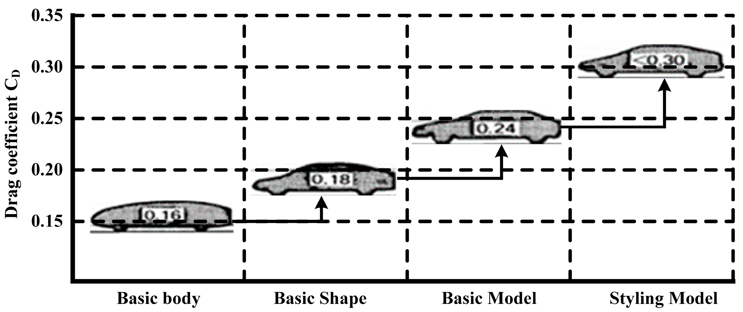
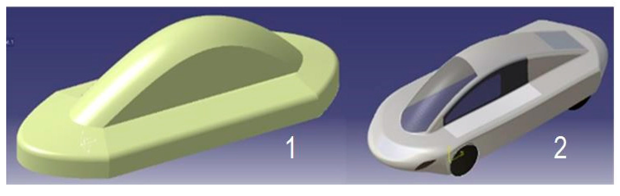
2.1. Vehicle Aerodynamics and Analysis

In order to analyze the flow of a body, it is necessary to solve the mass, momentum, and energy equations of the flow in contact with that object under the current boundary conditions. Equation (1) shows the aerodynamic drag force equation:

$$F_D=\underset{A}{\int }\left(p-p_{\propto }\right)d{A}_y$$

(1)

where $F_D$ is the aerodynamic drag force, $p$ is the ambient pressure, $p_{\propto }$ is the atmospheric pressure, and $A_y$ is the flow area perpendicular to the flow on the vehicle [44].

Based on Equation (2), the aerodynamic drag coefficient is found as follows:

$$C_D=\frac{F_D}{\frac{1}{2}\rho V^2{A}_f}$$

(2)

where $C_D$ is the aerodynamic drag coefficient, $\rho$ is the air density, $V$ is the air velocity, and $A_f$ is the front area of the vehicle [44].

The $C_D$ coefficient changes according to the shape of the vehicle and the angle of wind flow. A high $C_D$ coefficient is undesirable and should be reduced as much as possible for efficient driving. Decreasing the resistance force results in a reduction in energy consumption [44]. To improve the vehicle’s performance, its aerodynamics must be studied. The flow can be defined by using Navier–Stokes equations provided in Equations (3) and (4) [45]:

$$\frac{\partial \rho u_i}{\partial x_i}=0$$

(3)

$$\rho \left(u_f\frac{\partial u_i}{\partial x_j}\right)=-\frac{\partial p_i}{\partial x_i}+{\rho g}_i+\frac{\partial }{\partial x_j}\left[\mu \left(\frac{\partial u_i}{\partial x_j}+\frac{\partial u_j}{\partial x_i}\right)-\rho \overline{u_i^{\prime }{u}_j^{\prime }}\right]$$

(4)

where velocity indicates the $u_i$ components, and $\rho \overline{u_i^{\prime }{u}_j^{\prime }}$ indicates turbulent stresses. The analysis was carried out by assuming the flow as the steady state. These equations can be solved by using the Reynold’s-averaged Navier–Stokes equation (RANS) method.

The focus of this method is on the turbulence effect on average flow properties. It also solves the Navier–Stokes equation with approximate mean time and cannot solve all turbulent situations. $K-\epsilon$ and Reynolds stress models are the most well known in this solution technique. This method requires accurate flow calculations and considerable computational resources. Therefore, this approach has been the mainstay of engineering in flow calculations for the past thirty years [45].

In this study, the realizable $K-\epsilon$ turbulent flow model was selected from the RANS solution method. The modeled transport equations for $K$ and $\epsilon$ in the realizable model are shown in Equations (5) and (6):

$$\frac{\partial }{\partial t}\left(\rho k\right)+\frac{\partial }{\partial x_j}\left(\rho k{u}_j\right)=\frac{\partial }{\partial x_j}\left[\left(\mu +\frac{{\mu }_t}{{\sigma }_k}\right)\frac{\partial k}{\partial x_j}\right]+G_k+G_b-\rho \epsilon -Y_M+S_k$$

(5)

$$\frac{\partial }{\partial t}\left(\rho \epsilon \right)+\frac{\partial }{\partial x_j}\left(\rho \epsilon u_j\right)=\frac{\partial }{\partial x_j}\left[\left(\mu +\frac{{\mu }_t}{{\sigma }_k}\right)\frac{\partial \epsilon }{\partial x_j}\right]+\rho C_1{S}_{\epsilon }-\rho C_2\frac{{\epsilon }^2}{k+\sqrt{v\epsilon }}+C_{1\epsilon }\frac{\epsilon }{k}{C}_{3\epsilon }{G}_b+S_{\epsilon }$$

(6)

where Equation (7) is

$$C_1=max\left[0.43,\frac{\mathsf{\eta }}{\eta +5}\right], \eta =S\frac{k}{\epsilon }, S=\sqrt{2S_{ij}{S}_{ij}}$$

(7)

As with other $K-\epsilon$ models, the eddy viscosity (${\mu }_t$) was calculated from Equation (8).

$${\mu }_t=\rho C_{\mu }\frac{k^2}{\epsilon }$$

(8)

The difference between the realizable $K-\epsilon$ model and the standard and RNG $K-\epsilon$ models is that $C_{\mu }$ is no longer constant. Instead, it can be calculated from Equation (9):

$$C_{\mu }=\frac{1}{A_0+A_s\frac{k{U}^{*}}{\epsilon }}$$

(9)

where $U^{*}$ is provided in Equation (10) as follows:

$$U^{*}\equiv \sqrt{S_{ij}{S}_{ij}+{\tilde{\Omega }}_{ij}{\tilde{\Omega }}_{ij}}, {\tilde{\Omega }}_{ij}={\Omega }_{ij}-2{\epsilon }_{ij}{\omega }_k, {\Omega }_{ij}={\overline{\Omega }}_{ij}-{\epsilon }_{ijk}{\omega }_k$$

(10)

where ${\tilde{\Omega }}_{ij}$ is the mean rate-of-rotation tensor viewed in a moving reference frame with the angular velocity (${\omega }_k$). The model constants $A_0$ and $A_s$ are provided in Equation (11):

$$A_0=4.04, A_s=\sqrt{6}\cos \phi$$

(11)

where

$$\phi =\frac{1}{3}{\cos }^{-1}\left(\sqrt{6}W\right), W=\frac{S_{ij}{S}_{jk}{S}_{kj}}{{\tilde{S}}^3}, \tilde{S}=\sqrt{2S_{ij}{S}_{ij}}, S_{ij}=\frac{1}{2}\left(\frac{\partial u_j}{\partial x_i}+\frac{\partial u_i}{\partial x_j}\right)$$

(12)

It can be observed that $C_{\mu }$ is a function of the mean strain and rotation rates, the angular velocity of the system rotation, and the turbulence fields ($k$ and $\epsilon$). $C_{\mu }$ in Equation (9) can be shown to recover the standard value of 0.09 for an inertial sublayer in an equilibrium boundary layer. The model constants are provided as follows:

$$C_{1\epsilon }=1.44, C_2=1.9, {\sigma }_k=1.0, {\sigma }_{\epsilon }=1.2.$$

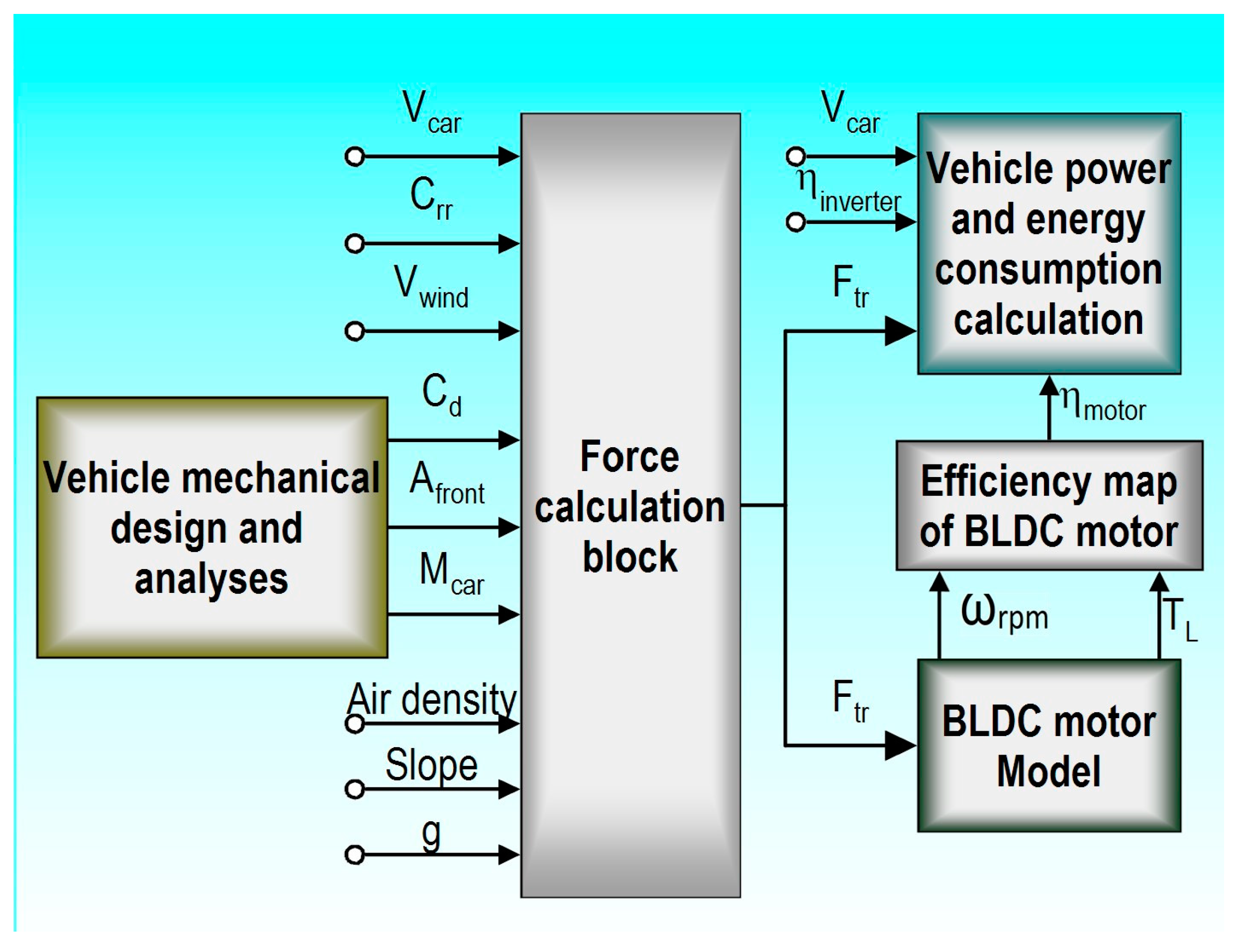
2.2. Vehicle Dynamic Modeling

The dynamic model of the designed EV was created using MATLAB–Simulink software. The route data utilized in the dynamic model correspond to the track specifically designated for lightweight EV prototype races in Korfez, Izmit, obtained via Google Earth 9.0 software. Figure 3a and Figure 3b depict the layout of the race track and its elevation profile, respectively.

2.2.1. PMSM Model

The voltage equations of the PMSM model are provided in Equation (13) [46]:

$$V_a=r_a{i}_a+\frac{{d\lambda }_a}{d_t}, V_b=r_b{i}_b+\frac{{d\lambda }_b}{d_t}, V_c=r_c{i}_c+\frac{{d\lambda }_c}{d_t}$$

(13)

where $V_a$, $V_b$, $V_c$ are phase-neutral voltages, ${\lambda }_a$, ${\lambda }_b$, ${\lambda }_c$ are the total fluxes of the phase windings, and $r_a$, $r_b$, $r_c$ are stator winding resistances [46].

If the total fluxes belonging to the windings are written as open, then Equation (14) is as follows [46]:

$$\begin{gathered} {\lambda }_a=L_{aa}{i}_a+L_{ab}{i}_b+L_{ac}{i}_c{+\lambda }_{ma} \\ {\lambda }_b=L_{ba}{i}_a+L_{bb}{i}_b+L_{bc}{i}_c{+\lambda }_{mb} \\ {\lambda }_c=L_{ca}{i}_a+L_{cb}{i}_b+L_{cc}{i}_c{+\lambda }_{mc} \end{gathered}$$

(14)

where $L_{aa}$, $L_{bb}$, and $L_{cc}$ are the self-inductances of the three-phase windings, and $L_{ab}$, $L_{ac}$, $L_{ba}$, $L_{bc}$, $L_{ca}$, and $L_{cb}$ are the mutual inductance between each three-phase winding. In addition, $i_a$, $i_b$, and $i_c$ are the currents of the three-phase windings, and ${\lambda }_{mi}$ is the total flux created by the magnets in the phase winding [46].

Generally, in PMSMs, since the magnets are placed on the rotor surface and the magnetic permeability of the magnets is close to the air magnetic permeability, it can be assumed that the position of the magnets does not affect the phase inductance. Moreover, if the stator structure is symmetrical, self-inductance and mutual inductance values can be considered constant [46]. In this case, if $L_{aa}$ = $L_{bb}$ = $L_{cc}$ = $L$, $L_{ab}$ = $L_{ac}$ = $L_{bc}$ = $M$ and the total flux equations are replaced by the voltage equations, then the voltage equation of phase A becomes Equation (15) [46].

$$V_a=r_a{i}_a+L\frac{{di}_a}{d_t}+M\frac{{di}_b}{d_t}+M\frac{{di}_c}{d_t}+\frac{{d\lambda }_{ma}}{d_t}$$

(15)

The matrix form of PMSM modeling equations is shown in Equation (16) [46].

$$\left[\begin{array}{c}{V}_a\\ V_b\\ V_c\end{array}\right]=\left[\begin{array}{ccc}{r}_a& 0& 0\\ 0& r_b& 0\\ 0& 0& r_c\end{array}\right]\left[\begin{array}{c}{I}_a\\ I_b\\ I_c\end{array}\right]+\left[\begin{array}{ccc}L-M& 0& 0\\ 0& L-M& 0\\ 0& 0& L-M\end{array}\right]\frac{d}{d_t}\left[\begin{array}{c}{I}_a\\ I_b\\ I_c\end{array}\right]+\left[\begin{array}{c}{e}_a\\ e_b\\ e_c\end{array}\right]$$

(16)

The electromagnetic power transferred to the rotor can be represented as Equation (17) [46].

$$P_e=e_a{i}_a+e_b{i}_b+e_c{i}_c$$

(17)

If it is assumed that all electromagnetic power is converted to kinetic energy when mechanical losses are ignored, the power is as in Equation (18) [46].

$$P_e=T_e{\mathsf{\omega }}_m$$

(18)

If (17) and (18) are combined, rotor speed can be obtained from Equation (19) [46].

$$T_e-T_L=j\frac{d{\mathsf{\omega }}_m}{d_t}+B{\mathsf{\omega }}_m$$

(19)

Since the designed motor back EMF waveform is sinusoidal, the motion voltage waveform function is defined as cosine. The motion voltages are shown in Equation (20) [46].

$$f_a\left(\mathsf{\theta }\right)=cos\left(\mathsf{\theta }\right), f_b\left(\mathsf{\theta }\right)=cos\left(\mathsf{\theta }-\frac{2\mathsf{\pi }}{3}\right), f_c(\mathsf{\theta })=cos(\mathsf{\theta }+\frac{2\mathsf{\pi }}{3})$$

(20)

The details of the designed PMSM model are shown in Figure 4.

2.2.2. PMSM Efficiency Map

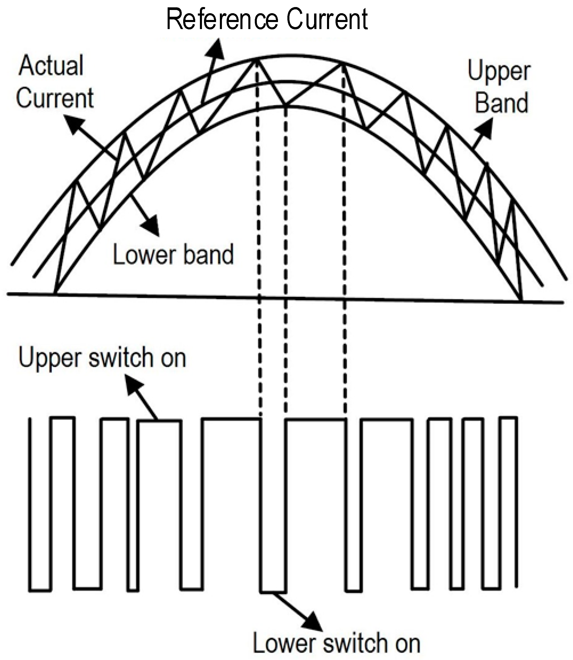
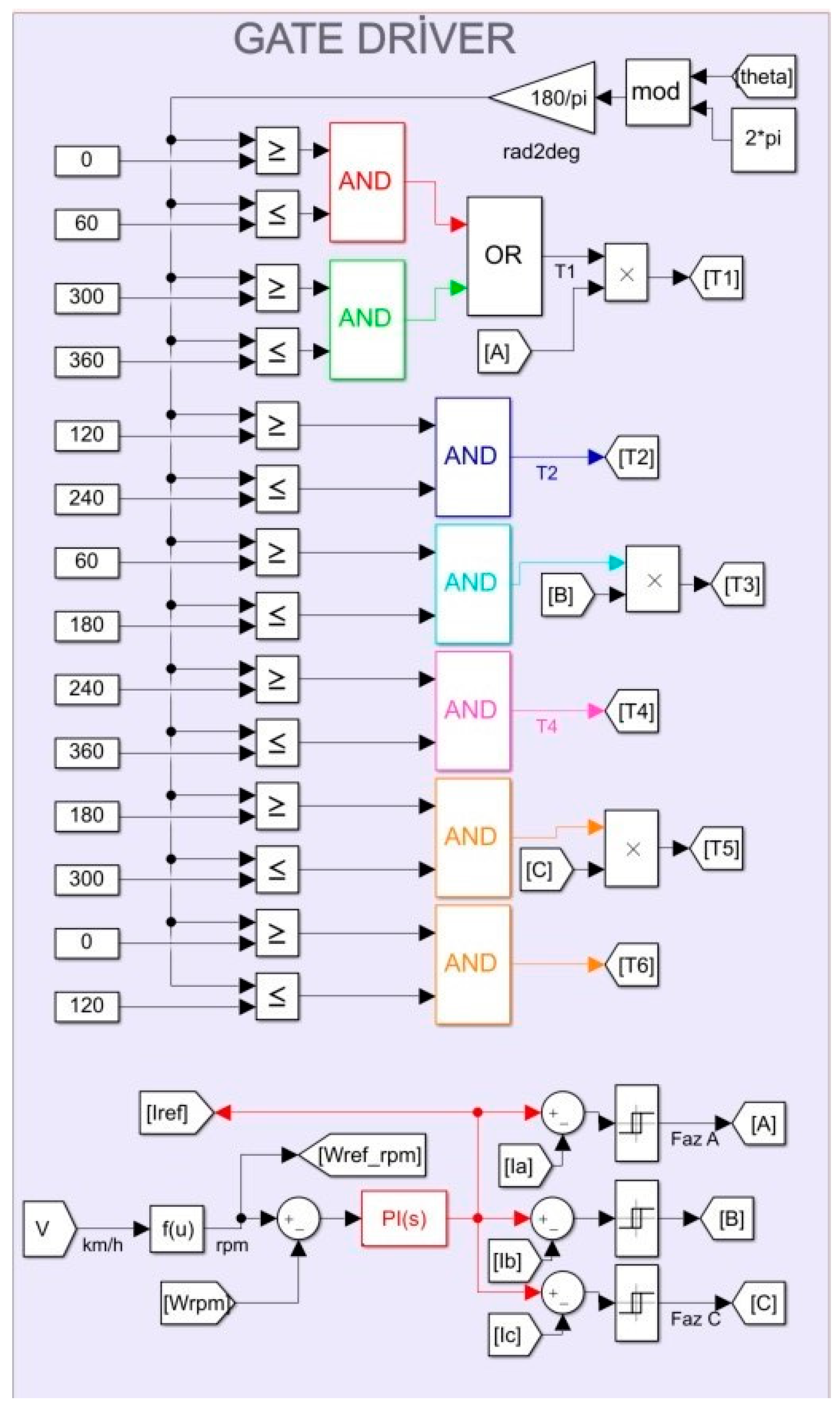
The parameters of the modeled PMSM belong to the motor designed and used for the vehicle, which competes in the TÜBİTAK efficiency challenge competition. A look-up table was created by transferring the yield map data of this motor to the MATLAB–Simulink environment. From here, the motor efficiency was calculated according to the motor speed and torque. Then, the efficiency value was used in the energy consumption calculation block. The PMSM efficiency map model is shown in Figure 5.

2.2.3. PMSM Driver

The hysteresis band current control technique is used to drive the PMSM. In the hysteresis band current control technique, the value of the current is forced to stay between certain limits, as shown in Figure 6.

In the PMSM Driver model, the reference current required for the existing conditions was found by using the PI controller. By using the hysteresis band block, the gate driving signals required to drive the upper switches of the A, B, and C phases are generated. The gate driver model is shown in Figure 7.

2.2.4. Force Calculation

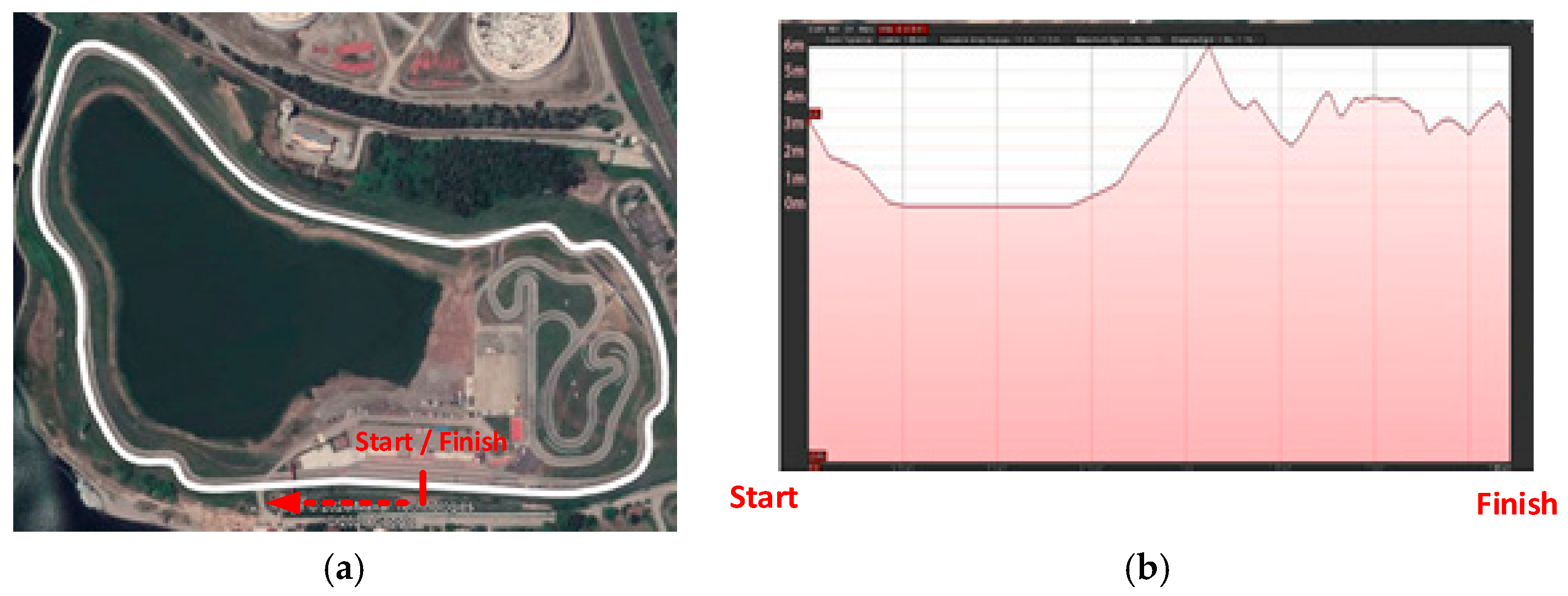
In this model, five different forces affecting the vehicle are calculated. According to Equation (21), the inertia force of the vehicle is calculated [47]:

$$f_I=M_{car}{·\dot{v}}_{car}$$

(21)

where $f_I$ indicates vehicle inertia force, $M_{car}$ indicates vehicle mass, and ${\dot{v}}_{car}$ indicates vehicle acceleration. In Equation (22), the gravitational force affecting the vehicle is calculated [47]:

$$f_g=M_{car}·g$$

(22)

where $f_g$ indicates gravitational force, and g indicates gravitational acceleration.

In Equation (23), the wheel rolling resistance force is calculated [47]:

$$f_{rr}=M_{car}·g·\mathit{cos}\left(\alpha \right)·c_{rr}$$

(23)

where $f_{rr}$ indicates the rolling resistance force of the wheels [N], $c_{rr}$ indicates the wheel rolling resistance coefficient, and $\alpha$ refers to the slope angle of the road.

The wind resistance force is calculated in Equation (24) [47].

$$f_{wind}=\frac{1}{2}·{\rho }_{air}·C_D·A_f·{(v_{car}+v_{wind})}^2$$

(24)

According to Equation (24), $f_{wind}$ indicates the wind resistance force [N], ${\rho }_{air}$ indicates dry air density at 20 °C [kg/m³], $C_D$ indicates the aerodynamic drag coefficient, $A_f$ indicates vehicle front area [m²], $v_{car}$ indicates vehicle speed [m/s], and $v_{wind}$ indicates wind speed [m/s] [47].

In Equation (25), the expression traction force affecting the vehicle is provided [47].

$$f_t=f_I+f_g·\mathrm{s}\mathrm{i}\mathrm{n}(\alpha )+{sign\left(v_{car}\right)f}_{rr}+{sign(v_{car}+v_{wind})f}_{wind}$$

(25)

3. Case Study

A detailed simulation is performed for two different vehicles and the results are shared for a realistic road map drive cycle to test the dynamic model.

The test procedure of the developed dynamic model requires an EV design stage. Hence, the shape design is carried out for two different vehicles. For a fair comparison, for both vehicles, the total mass and wheel friction coefficient are the same. The drivetrain components such as the electric motor, motor driver, and battery capacity are also the same.

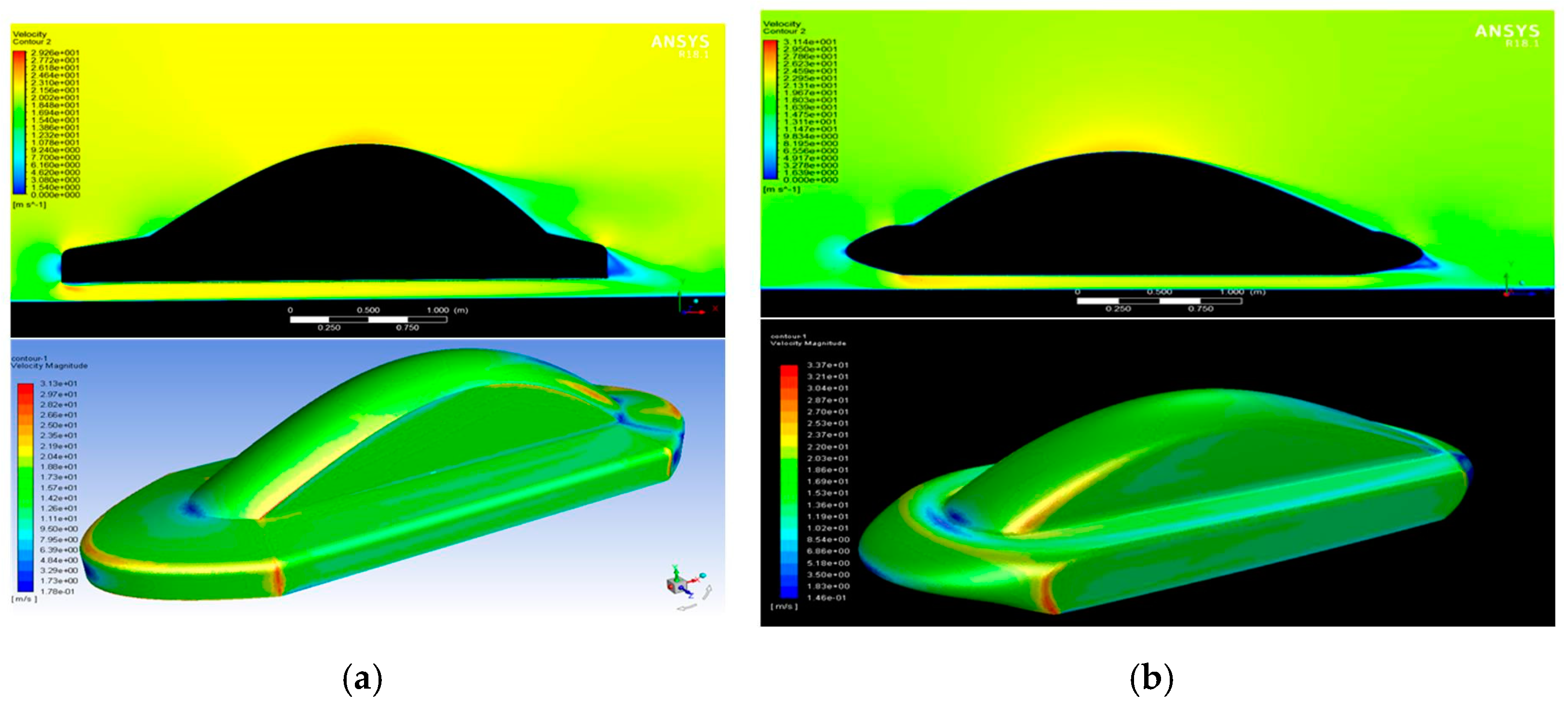
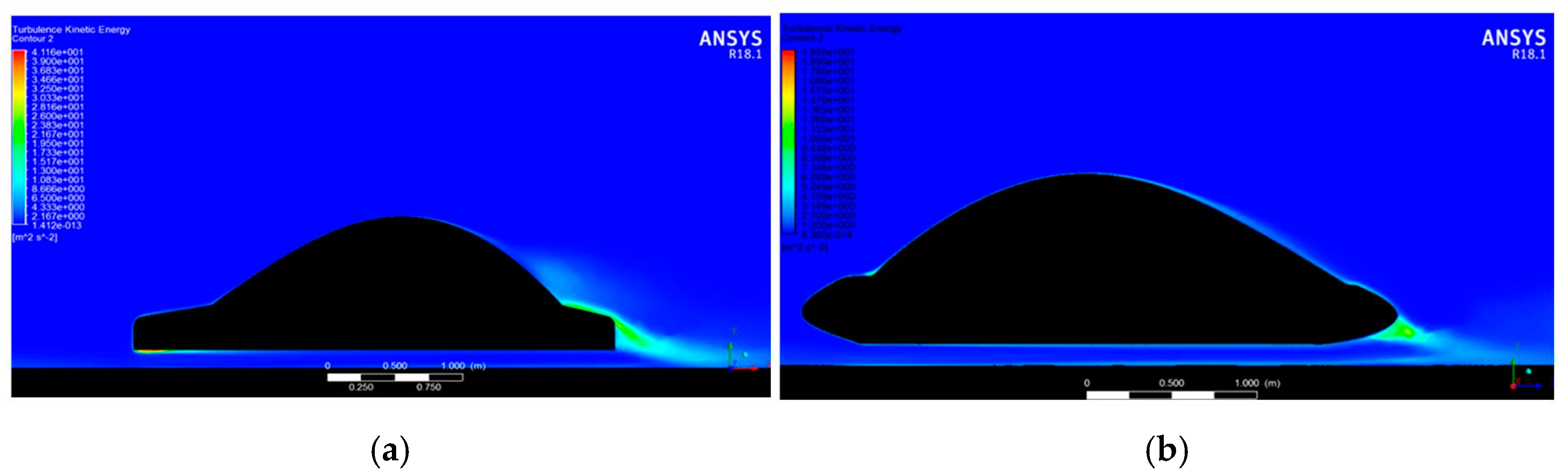
3.1. Aerodynamic Results

Vehicle designs were created using CATIA V5R21 software. These created designs were made solid for analysis. The aerodynamic analysis of the solidified designs was also conducted using ANSYS Fluent software. In the results obtained from these analyses, the shape of the flow over the design, velocity and pressure distributions, velocity vectors, streamlines, pressure coefficient distribution on the design, aerodynamic resistance, and lift coefficient affecting the design were calculated. Figure 8 shows the visual representations of the designed vehicles.

The main goal of designing two cars was to obtain different drag coefficients and lift coefficients from the aerodynamic study. For two different vehicle designs, analysis was performed by using ANSYS Fluent software at a constant speed of 72 km/h and the results were compared. The vehicle energy consumption was calculated using the C_d coefficient, weight of the vehicle, tire resistance, and area parameters obtained from the design results in the EV model prepared in the MATLAB environment. The results for vehicles 1 and 2 were compared. The designed vehicles are shown in Figure 8. The aerodynamic drag coefficients for vehicles 1 and 2 were approximately $C_{D1}=0.315$ and $C_{D2}=0.167$, respectively. The graphical representation illustrating the comparison of aerodynamic drag coefficients is depicted in Figure 9.

The aerodynamic lift coefficients for vehicles 1 and 2 were $C_{l1}=0.08$ and $C_{l2}=0.001$, respectively. Negative lift is very useful for improving cornering grip and is a desirable criterion for racing vehicles. According to Figure 9, the cornering grip of vehicle 2 is better. Figure 10 shows the velocity values for vehicles 1 and 2, respectively.

It can be observed in Figure 10 that the speed decreases toward the front and rear of the vehicle (blue zones) for both vehicles. The red-colored zones indicate places where the wind speed is high. The reason for the low speed in the front and rear parts is the high static pressure in these parts. On the other hand, the speed was high in the outer corners of the vehicles due to the static pressure being low in these parts. The highest velocities in the vehicles appeared in the lower-front part of the plane of symmetry. The lowest velocities in the vehicles appeared in the lower-rear part in the plane of symmetry. Figure 11 shows the turbulent kinetic energy impact on vehicles 1 and 2, respectively.

In Figure 11, it can be observed that turbulent kinetic energy density on the symmetry axis was high at the rear of both vehicles. Turbulent kinetic energy is related to vehicle speed. Therefore, speeds are high in the rear of the vehicles. Figure 12 shows the static pressure impact on vehicles 1 and 2.

In Figure 12, while the vehicle is moving, the airflow creates a force on the vehicle. This force increases the pressure in front of the vehicle. For both vehicles, the airflow increases the pressure as it moves through the hood. Airflow causes a pressure decrease on the upper part of the vehicle. This pressure decrease creates buoyancy due to the pressure difference above and below the vehicle. The lowest pressures on the vehicles occur where the speed of the vehicle is the highest.

3.2. Electrical Results

The waveform of the back EMF generated by using the PMSM mathematical model is illustrated in Figure 13. This graph serves as evidence that the motor model operates correctly. It is well known that low harmonic content in motor airgaps results in high efficiency and low torque ripple. However, sinusoidal back EMF not only provides high efficiency on the motor side, but it can also provide efficient inverter driving.

Considering the shape and elevation profile of the race track, a reference driving cycle has been established, as shown in Figure 14b. The speed control of the PMSM is carried out according to the driving cycle. The graph of reference speed and rotor speed is shown in Figure 14a. According to this figure, it is observed that the speed control of the PMSM is perfectly executed.

The PMSM load torque is calculated according to the traction force required for the vehicle to reach the reference speed. The force’s impact on the vehicle throughout the driving cycle is shown in Figure 15a. The load torque obtained according to these forces is shown in Figure 15b.

The data obtained from the efficiency map of the PMSM were processed in the MATLAB model and the instantaneous efficiency of the motor according to the speed and load torque of the motor was used in the model. The motor efficiency values drawn during the driving cycle were compared with the State of Charge (SoC) of the battery, as shown in Figure 16.

As can be observed in Figure 16, as the energy consumption of the vehicle decreases, the motor efficiency also decreases. However, due to the low energy consumption in this period, the impact of the motor efficiency on energy consumption is less. The voltage and current waveforms of the PMSM controlled by the hysteresis band control technique are provided in Figure 17. Figure 17a shows the three-phase current waveforms and Figure 17b shows the phase-to-phase voltage waveform.

Figure 17 delineates the features and attributes associated with the hysteresis band control technique employed for the PMSM. Conversely, Figure 18 portrays the comparison of the SoC values between the vehicles.

In Figure 18, it is apparent that the first instrument has a noticeably lower SoC value in comparison with the second. This discrepancy emphasizes the influential role of aerodynamic variables, such as the friction coefficient and the frontal area affected by the wind, in determining energy consumption. This comparison, involving vehicles of equal mass, accentuates how crucial these aerodynamic elements are in influencing the energy usage patterns within these vehicles.

4. Conclusions

The primary objective of this study was to evaluate the energy consumption of planned vehicle designs using a multidisciplinary approach and control strategy prior to the manufacturing phase. This investigation involved the analysis of two distinct vehicle designs under uniform external conditions such as road slope and wind speed. To estimate energy usage, dynamic vehicle models were constructed using MATLAB–Simulink, incorporating crucial performance parameters obtained from ANSYS Fluent, ANSYS Electronics, and CATIA, including $C_D$, $A_f$, and $M_{car}$.

The development of detailed models within MATLAB–Simulink encompassed the PMSM, its control algorithm, its efficiency map, and the equivalent friction force. By assessing the forces influencing the vehicles, calculations were made to determine the required traction force for wheel transmission within the dynamic models. This traction force facilitated the evaluation of load torque affecting the motor and the subsequent calculation of vehicle energy consumption. To regulate vehicle speed, a PI controller was utilized based on a predefined reference drive cycle intended for the race scenario. Analysis of load torque and speed data enabled the extraction of instantaneous efficiency data from the motor’s efficiency map. These efficiency parameters were integrated into the energy consumption model to compute the total energy expended by each vehicle. Subsequently, the battery model was discharged in accordance with the calculated energy consumption.

The study results indicated an energy consumption of 1124 Wh for the first vehicle and 632 Wh for the second vehicle, highlighting the superior efficiency of the latter design. Consequently, the second vehicle was selected for production and used in the competition. The research findings emphasize the necessity of a comprehensive, interdisciplinary analysis to evaluate the performance of lightweight EVs, encompassing factors such as Fluid Dynamics, tire frictions, drag coefficients, battery, motor, inverter, and other powertrain components. This study lays the groundwork for estimating energy consumption during the design phase of EVs. Notably, as the vehicle was intended for competition purposes, additional energy-consuming components such as lighting and air conditioning were intentionally omitted. Future investigations will aim to evaluate the influence of auxiliary components on energy consumption, contributing to the continuous improvement in vehicle efficiency. Additionally, in upcoming studies, integrating navigation during driving will facilitate real-time range predictions by considering the geographical features of the vehicle’s route.

References

1. Naik, S.C.; Ali, A.H.M.H.; Lobo, A.R.; Sona, S.S.; Badiger, M. A Comprehensive Review of Electric Vehicles: A Smart Choice for Environmental Sustainability and Energy Conservation; IGI Global: Hershey, PA, USA, 2024; ISBN 9798369326121. [Google Scholar]
2. Sun, X.; Li, Z.; Wang, X.; Li, C. Technology development of electric vehicles: A review. Energies 2019, 13, 90. [Google Scholar] [CrossRef]
3. Jose, P.S.; Jose, P.S.H.; Wessley, G.J.J.; Rajalakshmy, P. Environmental Impact of Electric Vehicles; Springer: Berlin/Heidelberg, Germany, 2022. [Google Scholar]
4. Emadi, A.; Lee, Y.J.; Rajashekara, K. Power electronics and motor drives in electric, hybrid electric, and plug-in hybrid electric vehicles. IEEE Trans. Ind. Electron. 2008, 55, 2237–2245. [Google Scholar] [CrossRef]
5. Jeong, M.-J.; Lee, K.-B.; Pyo, H.-J.; Nam, D.-W.; Kim, W.-H.; Jeong, M.-J.; Lee, K.-B.; Pyo, H.-J.; Nam, D.-W.; Kim, W.-H.A. A Study on the Shape of the Rotor to Improve the Performance of the Spoke-Type Permanent Magnet Synchronous Motor. Energies 2021, 14, 3758. [Google Scholar] [CrossRef]
6. Ahn, H.; Park, H.; Kim, C.; Lee, H. A Review of State-of-the-art Techniques for PMSM Parameter Identification. J. Electr. Eng. Technol. 2020, 15, 1177–1187. [Google Scholar] [CrossRef]
7. Li, X.; Williamson, S.S. Assessment of efficiency improvement techniques for future power electronics intensive hybrid electric vehicle drive trains. In Proceedings of the 2007 IEEE Canada Electrical Power Conference, EPC 2007, Montreal, QC, Canada, 25–26 October 2007; IEEE: Piscataway, NJ, USA, 2007; pp. 268–273. [Google Scholar]
8. Sagar, A.; Kashyap, A.; Nasab, M.A.; Padmanaban, S.; Bertoluzzo, M.; Kumar, A.; Blaabjerg, F. A Comprehensive Review of the Recent Development of Wireless Power Transfer Technologies for Electric Vehicle Charging Systems. IEEE Access 2023, 11, 83703–83751. [Google Scholar] [CrossRef]
9. Wang, W.; Chen, X.; Wang, J. Motor/Generator Applications in Electrified Vehicle Chassis-A Survey. IEEE Trans. Transp. Electrif. 2019, 5, 584–601. [Google Scholar] [CrossRef]
10. Pindoriya, R.M.; Rajpurohit, B.S.; Kumar, R.; Srivastava, K.N. Comparative analysis of permanent magnet motors and switched reluctance motors capabilities for electric and hybrid electric vehicles. In Proceedings of the 2018 IEEMA Engineer Infinite Conference, eTechNxT 2018, New Delhi, India, 13–14 March 2018; Institute of Electrical and Electronics Engineers Inc.: Piscataway, NJ, USA, 2018; pp. 1–5. [Google Scholar]
11. Li, W.; Wan, Y. Classical Electric Machines for Electric and Hybrid Vehicles; Springer: Singapore, 2024; Volume Part F2211. [Google Scholar]
12. Eldho Aliasand, A.; Josh, F.T. Selection of Motor foran Electric Vehicle: A Review. Mater. Today: Proc. 2020, 24, 1804–1815. [Google Scholar] [CrossRef]
13. Liu, X.; Chen, H.; Zhao, J.; Belahcen, A. Research on the Performances and Parameters of Interior PMSM Used for Electric Vehicles. IEEE Trans. Ind. Electron. 2016, 63, 3533–3545. [Google Scholar] [CrossRef]
14. Estima, J.O.; Marques Cardoso, A.J. Efficiency analysis of drive train topologies applied to electric/hybrid vehicles. IEEE Trans. Veh. Technol. 2012, 61, 1021–1031. [Google Scholar] [CrossRef]
15. Chirca, M.; Dranca, M.A.; Breban, S.; Oprea, C.A. PMSM Evaluation for Electric Drive Train for L6e Light Electric Vehicles. In Proceedings of the EPE 2020—Proceedings of the 2020 11th International Conference and Exposition on Electrical and Power Engineering, Iasi, Romania, 22–23 October 2020; Institute of Electrical and Electronics Engineers Inc.: Piscataway, NJ, USA, 2020; pp. 211–216. [Google Scholar]
16. Zhang, H.; Wang, Y.; Hua, W.; Gerada, D.; Cheng, M. Analysis of the Flux Density and Back EMF in Eccentric Permanent Magnet Machines Based on 2-D Air-Gap Modulation Theory. IEEE Trans. Transp. Electrif. 2022, 8, 4325–4336. [Google Scholar] [CrossRef]
17. Polat, M.; Yildiz, A.; Akinci, R. Performance Analysis and Reduction of Torque Ripple of Axial Flux Permanent Magnet Synchronous Motor Manufactured for Electric Vehicles. IEEE Trans. Magn. 2021, 57, 1–9. [Google Scholar] [CrossRef]
18. Shahina, S.; Muhammed, F. Review of Speed Controlling Techniques on Dual PMSM Drive Systems. In Proceedings of the International Conference on Futuristic Technologies in Control Systems and Renewable Energy (ICFCR 2022), Malappuram, India, 21–22 July 2022. [Google Scholar]
19. Keskin Arabul, F.; Senol, I.; Oner, Y. Performance Analysis of Axial-Flux Induction Motor with Skewed Rotor. Energies 2020, 13, 4991. [Google Scholar] [CrossRef]
20. Guan, Y.; Zhu, Z.Q.; Afinowi, I.A.A.; Mipo, J.C.; Farah, P. Comparison between induction machine and interior permanent magnet machine for electric vehicle application. Compel-Int. J. Comput. Math. Electr. Electron. Eng. 2016, 35, 572–585. [Google Scholar] [CrossRef]
21. Kose, O.; Oktay, T. Simultaneous quadrotor autopilot system and collective morphing system design. Aircr. Eng. Aerosp. Technol. 2020, 92, 1093–1100. [Google Scholar] [CrossRef]
22. Mushid, F.C.; Dorrell, D.G. Review of axial flux induction motor for automotive applications. In Proceedings of the 2017 IEEE Workshop on Electrical Machines Design, Control and Diagnosis, WEMDCD 2017, Nottingham, UK, 20–21 April 2017; Institute of Electrical and Electronics Engineers Inc.: Piscataway, NJ, USA, 2017; pp. 146–151. [Google Scholar]
23. Cao, Z.; Mahmoudi, A.; Kahourzade, S.; Soong, W.L. An Overview of Axial-Flux Induction Machine. In Proceedings of the 2021 31st Australasian Universities Power Engineering Conference, AUPEC 2021, Perth, Australia, 26–30 September 2021; Institute of Electrical and Electronics Engineers Inc.: Piscataway, NJ, USA, 2021; pp. 1–6. [Google Scholar]
24. Bitsi, K.; Bosga, S.G. A Case Study of Pole-Phase Changing Induction Machine Performance. In Proceedings of the 24th European Conference on Power Electronics and Applications, EPE 2022 ECCE Europe, Hanover, Germany, 5–9 September 2022. [Google Scholar]
25. Garip, S.; Yasa, Y. Design of Outer Runner-Type Brushless Permanent Magnet DC Motor for Lightweight E-Vehicles. In Proceedings of the 2020 6th International Conference on Electric Power and Energy Conversion Systems, EPECS 2020, Istanbul, Turkey, 5–7 October 2020; Institute of Electrical and Electronics Engineers Inc.: Piscataway, NJ, USA, 2020; pp. 151–156. [Google Scholar]
26. Hucho, W.H.; Sovran, G. Aerodynamics of road vehicles. Annu. Rev. Fluid Mech. 1993, 25, 485–537. [Google Scholar] [CrossRef]
27. Damjanović, D.; Kozak, D.; Živić, M.; Ivandić, Ž.; Baškarić, T. CFD analysis of concept car in order to improve aerodynamics. Járműipari Innováció 2011, 1, 108–115. [Google Scholar]
28. Koenig-Fachsenfeld, R.V.; Ruehle, D.; Eckert, A.; Zeuner, M. Windkanalmessungen an Omnibusmodellen. ATZ 1936, 39, 143–149. [Google Scholar]
29. Anderson, J.D.; Wendt, J. Computational Fluid Dynamics; Springer: New York, NY, USA, 1995. [Google Scholar]
30. Ansys Inc. ANSYS CFX User’s Guide; Ansys Inc.: Kirkland, WA, USA, 2017. [Google Scholar]
31. Hetawal, S.; Gophane, M.; Ajay, B.K.; Mukkamala, Y. Aerodynamic Study of Formula SAE Car. Procedia Eng. 2014, 97, 1198–1207. [Google Scholar] [CrossRef]
32. Hinterberger, C.; García-Villalba, M.; Rodi, W. Large eddy simulation of flow around the Ahmed body. Aerodyn. Heavy Veh. Truck. Buses Trains. Lect. Notes Appl. Comput. Mech. 2004, 19, 77–87. [Google Scholar] [CrossRef]
33. Ahmed, S.R.; Ramm, G.; Faltin, G. Some Salient Features of the Time -Averaged Ground Vehicle Wake. SAE Trans. SAE Int. 1984, 93, 473–503. [Google Scholar]
34. Miri, I.; Fotouhi, A.; Ewin, N. Electric vehicle energy consumption modelling and estimation—A case study. Int. J. Energy Res. 2021, 45, 501–520. [Google Scholar] [CrossRef]
35. Hong, J.; Park, S.; Chang, N. Accurate remaining range estimation for Electric vehicles. In Proceedings of the Asia and South Pacific Design Automation Conference, ASP-DAC, Macao, China, 25–28 January 2016; IEEE: Piscataway, NJ, USA, 2016; pp. 781–786. [Google Scholar]
36. Kim, D.M.; Jung, Y.H.; Cha, K.S.; Lim, M.S. Design of Traction Motor for Mitigating Energy Consumption of Light Electric Vehicle Considering Material Properties and Drive Cycles. Int. J. Automot. Technol. 2020, 21, 1391–1399. [Google Scholar] [CrossRef]
37. Wu, X.; Freese, D.; Cabrera, A.; Kitch, W.A. Electric vehicles’ energy consumption measurement and estimation. Transp. Res. Part D Transp. Environ. 2015, 34, 52–67. [Google Scholar] [CrossRef]
38. Fiori, C.; Ahn, K.; Rakha, H.A. Power-based electric vehicle energy consumption model: Model development and validation. Appl. Energy 2016, 168, 257–268. [Google Scholar] [CrossRef]
39. De Cauwer, C.; Van Mierlo, J.; Coosemans, T. Energy Consumption Prediction for Electric Vehicles Based on Real-World Data. Energies 2015, 8, 8573–8593. [Google Scholar] [CrossRef]
40. Zhang, R.; Yao, E. Electric vehicles’ energy consumption estimation with real driving condition data. Transp. Res. Part D Transp. Environ. 2015, 41, 177–187. [Google Scholar] [CrossRef]
41. De Cauwer, C.; Verbeke, W.; Coosemans, T.; Faid, S.; Van Mierlo, J. A Data-Driven Method for Energy Consumption Prediction and Energy-Efficient Routing of Electric Vehicles in Real-World Conditions. Energies 2017, 10, 608. [Google Scholar] [CrossRef]
42. Kriesel, D. A Brief Introduction on Neural Networks; Citeseer: Princeton, NJ, USA, 2007. [Google Scholar]
43. Qi, X.; Wu, G.; Boriboonsomsin, K.; Barth, M.J. Data-driven decomposition analysis and estimation of link-level electric vehicle energy consumption under real-world traffic conditions. Transp. Res. Part D Transp. Environ. 2018, 64, 36–52. [Google Scholar] [CrossRef]
44. Erzi, A.I. Tasit Teknigi-Ders Notlari; ITU Makina Fakultesi: Istanbul, Türkiye, 1998. [Google Scholar]
45. Versteeg, H.K.; Malalasekera, W. An Introduction to Computational Fluid Dynamics: The Finite Volume Method; Pearson Education: London, UK, 2007. [Google Scholar]
46. Wu, H.X.; Cheng, S.K.; Cui, S.M. A controller of brushless DC motor for electric vehicle. IEEE Trans. Magn. 2005, 41, 509–513. [Google Scholar] [CrossRef]
47. Schaltz, E. Electrical Vehicle Design and Modeling, 1st ed.; Soylu, S., Ed.; InTech: Rijeka, Croatia, 2011. [Google Scholar]
Figure 1. Variation in drag coefficient according to vehicle body shape [28].
Sustainability 16 04928 g001
Figure 2. The principal scheme of the dynamic model.
Sustainability 16 04928 g002
Figure 3. (a) Race track route; (b) elevation profile of the race track.
Sustainability 16 04928 g003
Figure 4. PMSM model.
Sustainability 16 04928 g004
Figure 5. PMSM efficiency map model.
Sustainability 16 04928 g005
Figure 6. Hysteresis band control technique.
Sustainability 16 04928 g006
Figure 7. PMSM gate driver model.
Sustainability 16 04928 g007
Figure 8. Representation of two different vehicle designs illustrating the variations in their aerodynamic properties.
Sustainability 16 04928 g008
Figure 9. (a) Aerodynamic drag coefficient graph; (b) lift coefficient graph.
Sustainability 16 04928 g009
Figure 10. Velocity values of the vehicle designs: (a) vehicle 1; (b) vehicle 2.
Sustainability 16 04928 g010
Figure 11. Turbulent kinetic energy impacts on the vehicle designs: (a) vehicle 1; (b) vehicle 2.
Sustainability 16 04928 g011
Figure 12. Static pressure impact on the vehicle designs: (a) vehicle 1; (b) vehicle 2.
Sustainability 16 04928 g012
Figure 13. The back EMF waveform of the designed PMSM.
Sustainability 16 04928 g013
Figure 14. (a) Comparing reference and rotor speed graphs. (b) Driving cycle for a lap.
Sustainability 16 04928 g014
Figure 15. (a) The force impact on the vehicle; (b) load torque of the BLDC motor.
Sustainability 16 04928 g015
Figure 16. (a) Load torque of the PMSM; (b) efficiency of the PMSM.
Sustainability 16 04928 g016
Figure 17. Waveforms of the PMSM: (a) current waveforms; (b) voltage waveforms.
Sustainability 16 04928 g017
Figure 18. Comparison of the SoC values of the vehicles.
Sustainability 16 04928 g018
Disclaimer/Publisher’s Note: The statements, opinions and data contained in all publications are solely those of the individual author(s) and contributor(s) and not of MDPI and/or the editor(s). MDPI and/or the editor(s) disclaim responsibility for any injury to people or property resulting from any ideas, methods, instructions or products referred to in the content.