Variations of Global Compound Temperature and Precipitation Events and Associated Population Exposure Projected by the CMIP6 Multi-Model Ensemble

Abstract

Compound climate events often pose greater harm to humans and society than single-variable climate issues. This study projects the temporal changes and spatial pattern evolution of four compound climate events (including warm–wet, warm–dry, cold–wet, and cold–dry) and the corresponding population exposure in global land under the shared socioeconomic pathway (SSP) 2–4.5 based on the Coupled Model Intercomparison Project phase 6 simulations. Results show the following: (1) The warm–wet event is significantly decreasing at a rate of 0.06 days per decade, while the cold–wet event is significantly increasing at a rate of 0.06 days per decade. The warm–dry event and cold–dry event show an upward trend but are not significant. (2) All four types of compound events will undergo mutations in the next 80 years, with the warm–dry event having the highest frequency of mutations. (3) West Asia is a high-risk area for warm–dry and cold–wet events. Northern Africa is a hot spot area for the warm–wet event, while Brazil is a hot spot area for the cold–dry event. (4) Areas with exposure levels (population under four compound climate events) of medium or higher are mainly distributed in East Asia, South Asia, and central Africa. When the population exposure exceeds 10⁵ person · day, the area of population exposure to compound events related to dry conditions is greater than that of compound events related to wet conditions. This study has guiding significance for understanding, identifying, analyzing, and preventing compound extreme climate events in the context of global warming.

1. Introduction

Climate change is an extremely important part of global change, and extreme climate events seriously affect human activities and life safety [1,2,3,4]. For instance, in the summer of 2003, a heatwave occurred on the European continent, resulting in approximately 30,000 deaths [5]. In 2013, an extreme heatwave in southeastern China broke a 140-year record, with 167 deaths in Pudong New Area alone, with particularly severe injuries in elderly people and women [6]. In the middle of September 2019, the rainstorm brought by the tropical storm triggered large-scale floods in Texas, USA, and nearly 6.6 million people were affected [7]. These extreme events have received widespread attention due to the serious harm they cause. Some scholars have conducted research on their spatial distribution pattern, characteristics of time series, center-of-gravity movement direction, and formation mechanism [8,9,10,11].

Climate change is an increasingly likely combination of extreme events that were previously considered unlikely to occur. With the intensification of global warming, the likelihood of composite extreme events occurring in many regions will become more frequent [12,13]. For example, the variable of near-surface temperature cannot accurately describe the intensity and impact of extreme heat events. The human body mainly dissipates its own heat load through sweating in hot environments. If the surrounding humidity is high at this time, the human body’s heat dissipation ability will decrease [14,15]. Therefore, compound extreme heat events with high temperature and high humidity can pose more serious hazards to human health. In 2010, Russia experienced simultaneous occurrences of minimal precipitation and extremely hot conditions, leading to widespread wildfires, damaging crops, and leading to human death [16,17,18,19]. The sixth assessment report of the Intergovernmental Panel on Climate Change (IPCC AR6) pointed out that the global temperature is expected to rise to or exceed 1.5 °C in the next 20 years, and the probability of compound extreme weather events will increase [20]. Considering the high destructiveness of composite extreme climate events and their strong impact on humans, predicting the spatiotemporal changes of future composite extreme climate events is extremely important in order to address climate risks and prevent significant health or economic losses to humans.

Temperature and precipitation are two variables that cannot be ignored in climate science and hydrological research, and are commonly used to evaluate research on compound extreme events [21]. Typically, the combination of extreme high temperature and drought has had catastrophic impacts on the ecological environment, such as crop yield reduction [22], increased tree mortality [23], and impacts on human life and health [24]. Other compound situations, such as the simultaneous occurrence of high temperature and heavy rainfall, may lead to the occurrence of floods (e.g., Scandinavia and Norway) and have a serious impact on society [25,26]. Given the above issues, a deep understanding of the changes in different types of compound temperature and precipitation events is crucial in order to take appropriate measures to reduce the potential impact of climate change on society. However, the assessment of future changes in different types of compound temperature and precipitation events on a global scale is extremely limited.

At present, the projection data of the Coupled Model Intercomparison Project phase 6 (CMIP6) have been publicly released. Compared with previously released models, the CMIP6 model has more detailed physical processes and a higher spatial resolution [27,28]. The goal of this study is to predict the temporal and spatial changes of different types of compound temperature and precipitation events worldwide based on the CMIP6 simulation. Considering that population exposure is a crucial factor in disaster risk assessment [29], we also simulated the corresponding population exposure situations under different compound events. The chapter arrangement is as follows: Section 2 introduces the data sources and research methods. Section 3 describes the experimental results. The discussion and reflection on the results are laid out in Section 4. The final chapter presents the conclusions of this study.

2. Materials and Methods

2.1. Source of Data

In this study, the calculation of the compound extreme climate indices mainly used three types of data: daily precipitation, daily maximum temperature, and daily minimum temperature. Considering the resolution of the model, we selected five GCMs models with relatively complete data and higher resolution from the Sixth Coupled Comparison Plan (CMIP6), and the basic information (data available at https://esgf-node.llnl.gov/projects/cmip6/, accessed on 1 September 2023) is shown in

Table 1. GCMs’ basic information.

Number	Name	Country	Original Resolution
1	GFDL-ESM4	USA	1° × 1.25°
2	UKESM1-0-LL	UK	1.875° × 1.25°
3	MPI-ESM1-2-HR	Germany	0.93° × 0.94°
4	IPSL-CM6A-LR	France	1.27° × 2.5°
5	MRI-ESM2-0	Japan	1.125° × 1.125°

.

Before conducting calculations, we set the future as a medium emission scenario, and the social response to climate change risk is medium vulnerability, so we ultimately adopted the SSP2-4.5 scenario in CMIP6. This scenario is an updated version of RCP4.5 in CMIP5. It belongs to the medium radiative forcing scenario, and the radiative forcing will be stable at about 4.5 W/m² in 2100 [30]. This scenario is often used as a reference for CMIP6, such as the Regional Downscaling and Interdecadal Climate Prediction Program (DCCP) in the Collaborative Regional Climate Downscaling Program (CORDEX).

Considering the different resolutions between different modes (climate data produced by different countries or institutions), we first use the bilinear interpolation method to uniformly interpolate all mode data, and the final resolution is 0.5° × 0.5°. Then, we adopted the method of averaging to reduce the errors caused by different modes.

2.2. Definition of Compound Indices

Following the definition of complex extreme climate events in previous studies [31,32], we use the 25th and 75th percentile of temperature and precipitation as the threshold to divide warm/cold and wet/dry. The compound indices definition we used in this experiment is shown in

Table 2. Definition of compound indices.

Name	Definition	Units
warm–wet	Tmax > T75 & P > P75	d
warm–dry	Tmax > T75 & P < P25	d
cold–wet	Tmin < T25 & P > P75	d
cold–dry	Tmin < T25 & P < P25	d

.

The meanings of each code are as follows: T_max represents the daily maximum temperature, T_min represents the daily minimum temperature, P represents the daily precipitation, T₇₅ represents the 75th quantile of the daily maximum temperature of each year, T₂₅ represents the 25th quantile of the daily minimum temperature of each year, P₇₅ represents the 75th quantile of the daily precipitation of each year, and P₂₅ represents the 25th quantile of the daily precipitation of each year.

2.3. Trend Testing and Mutation Analysis

M-K test is widely used in hydrology, meteorology, environmental science, and other disciplines by many scholars [33,34]. It allows a small number of outliers, and does not require samples to follow a specific distribution pattern. Therefore, this experiment uses the non-parametric Mann–Kendall (M-K) method to test the future trend and whether there is a sudden change in the compound extreme climate indices [35,36]. The calculation steps of this method are as follows:

For a series with n sample size, $R_i$ represents that the i-th sample $x_i$ of the sequence is greater than the cumulative number of $x_j$ (1 ≤ $j$ ≤ $i$); then, the statistic $s_k$ is as follows:

$$s_k={\sum }_{i=1}^k{R}_i \left(k=2 ,3,\dots ,n\right)$$

(1)

Assuming that this time series is random and independent, the connotation of $UF$ is as follows:

$$UF=\frac{s_k-E\left(s_k\right)}{\sqrt{Var\left(s_k\right)}} \left(k=2, 3,\dots ,n\right)$$

(2)

$$E(s_k)=\frac{n(n+1)}{4}$$

(3)

$$\sqrt{Var\left(s_k\right)}=\frac{n(n-1)(2n+5)}{72}$$

(4)

where $E\left(s_k\right)$ and $Var\left(s_k\right)$ are the mean and variance, respectively, of $s_k$. The above process is repeated while making $UB$ = −$UF$ ($k=n,n-1,\dots ,1$).

$UF$ is the standard normal distribution. At the significance level α (generally taken as α = 0.05, $U_{\mathsf{\alpha }}$ = ±1.96), if |$UF$| > |$U_{\mathsf{\alpha }}$|, it indicates that there is an obvious trend of increase or decrease in the sequence. If the $UB$ and $UF$ curves intersect between two adjacent boundaries, we assume that the time corresponding to the intersection point on the horizontal axis is the time when the mutation occurred.

2.4. Global Spatial Autocorrelation Analysis

In this study, we use the global Moran’s I to judge whether the four compound extreme climate events are spatially autocorrelated. In other words, if a region is a high-risk area for a compound event, is the surrounding area also a high-risk area for that event? Is there no spatial correlation between the number of occurrences of an event in the region and the surrounding area? Spatial autocorrelation refers to the spatial dependence of observed variables, that is, whether variables with similar spatial locations have similar or opposite trends. The most commonly used statistic is Moran’s I index with range of [−1, 1] [37]. When the index is greater than zero and reaches a significant level, the global spatial autocorrelation is positive. The larger the value, the more obvious the spatial aggregation; when the index is less than zero, the global spatial autocorrelation is a negative correlation. The closer to −1, the higher the degree of spatial negative correlation; when the index is zero, it means that the observed variable has no spatial correlation, that is, random spatial distribution [38]. The calculation formula is as follows:

$$I=\frac{n\sum _{i=1}^n\sum _{j=1}^n{w}_{ij}\left(x_i-\overline{x}\right)\left(x_j-\overline{x}\right)}{\left(\sum _{i=1}^n\sum _{j=1}^n{w}_{ij}\right)\sum _{i=1}^n{\left(x_i-x\right)}^2}$$

(5)

$$\overline{x}=\frac{1}{n}{\sum }_{i=1}^n{x}_i$$

(6)

In the above equation: $x_i$ and $x_j$ represent the values of indices for two geographical units, respectively. And $w_{ij}$ represents the spatial weight value. In this study, we use a binary adjacency matrix to define the proximity relationship between two geographical units. That is, when two geographical units are adjacent, the value is 1, and, when they are not adjacent, the value is 0. The statistical significance of Moran’s I is commonly transformed to a Z-score test with a standard normal distribution [39]:

$$Z(I)=\frac{I-E\left(I\right)}{\sqrt{Var\left(I\right)}}$$

(7)

where $E\left(I\right)$ is the expected value of $I$ for a random spatial pattern, and $Var\left(I\right)$ represents the variance of $I$. A positive $Z$-score with a significant level implies that the distribution of the extreme hot index is spatially clustered. A significance level of 0.05 was used in our study.

2.5. Hot Spot and Cold Spot Analysis

The hot spot analysis method can identify high-value (hot spot) and low-value (cold spot) regions of geographical objects, which are statistically significant spatial clusters [40]. This method can be used to estimate and understand the spatial distribution pattern and pattern of global compound extreme events. Geographic units with high Z-score and small p-value indicate statistically significant hot spots, and those with low negative Z-score and small p-value demonstrate statistically significant cold spots [41,42]. The principle of this index is as follows:

$$G_i(d)=\frac{\sum _{j=1}^n{w}_{ij}\left(d\right)x_j}{\sum _{j=1}^n{x}_j}$$

(8)

where $w_{ij}\left(d\right)$ is the weight matrix within the range of distance ($i$ ≠ $j$). We use the face adjacency model from the ArcMap toolbox (with adjacent nodes, edges, and intersecting face data) to calculate the spatial weight matrix. $G_i\left(d\right)$ represents the degree of correlation between the statistics of province $i$ and the neighboring province $j$ under the condition of distance weight $w_{ij}\left(d\right)$. The formula for standardization of $G_i\left(d\right)$ is:

$${Z(G}_i)=\frac{\left[G_i\right(d\left)\right]-E\left(G_i\right)}{\sqrt{VAR\left(G_i\right)}}$$

(9)

where the $E\left(G_i\right)$ and $VAR\left(G_i\right)$ represent the mathematical expectation and theoretical variance of $G_i$, respectively. ${Z(G}_i)$ is positive and significant, indicating that the value of extreme hot around station i is high, so station i belongs to the hot spot area; ${Z(G}_i)$ is negative and significant, indicating that the value of extreme hot around station i is low, so it belongs to the cold spot area. Identifying and plotting the hot and cold spot areas of four compound events can lead us to intuitively perceive areas susceptible to climate disasters in space, which is of great significance for relevant departments in order to deploy corresponding policies in advance to achieve the goal of disaster prevention and reduction.

2.6. Calculation of Population Exposure

We calculated the exposure levels of the population under different composite events in 2060 and 2100. The exposure level of a certain area is defined as the product of the number of days that extreme events occur in that area and the population of that area [43]. The population data in this study come from the International Institute for Applied Systems Analysis (IIASA), which takes into account local population policies and uses spatial econometric models for estimation [44]. The detailed address for obtaining data is: https://sedac.ciesin.columbia.edu/data/set/gpw-v4-population-count-adjusted-to-2015-unwpp-country-totals-rev11 (accessed on 1 September 2023).

3. Results

3.1. The Temporal Variation Pattern of Compound Extreme Events

We calculated the changes of four compound extreme climate indices from 2020 to 2100, as shown in Figure 1. We can see that, on a global scale, cold–dry events occur for about 30 days a year, with a maximum of 30.79 days in 2020 and a minimum of 29.21 days in 2039. The warm–wet events occur for approximately 24 days per year, with a maximum of 25.36 days in 2046 and a minimum of 23.85 days in 2044. The warm–dry event has nearly 21 days in a year, with a maximum of 22.69 days in 2022 and a minimum of 20.93 days in 2098. The cold- wet events occur for approximately 15 days per year, with a maximum of 15.72 days in 2081 and a minimum of 14.45 days in 2020.

In order to further understand the differences between the values of the four compound extreme climate events in each year and the average values in the past 80 years, and to observe the fluctuations of the values around the average values in each year, we calculated the anomalies of the four compound extreme climate indices in the next 80 years (Figure 2). In the next 80 years, the anomalous values of warm–wet events will exceed the average for 39 years, and the average values during the first 40 years (2020–2060) will be significantly higher than those in the latter 40 years (2061–2100). The average value of this event is 24.61 days in the next 80 years. The average value of cold–wet events is 15.06 days, which is the opposite to that of warm–wet events. The average value of this event in the next 40 years is higher than that in the first 40 years. In the next 80 years, the average value of warm–dry events is 21.61 days. There are 37 years in which the anomaly value of this event is greater than 0, and the average value in the next 40 years is greater than that in the first 40 years. There are 41 years in which the anomaly value of the cold–dry event is greater than 0, with an average of 30.15 days. In the next 40 years, there will be more years with an anomaly value greater than 0 than in the first 40 years.

We use the M-K test to verify whether there are significant changes in the time series of four compound extreme climate events, and the test results are shown in

Table 3. M-K test results of four compound indices.

	Warm–Wet	Cold–Wet	Warm–Dry	Cold–Dry
z	−3.98	4.64	0.35	1.26
p	<0.01	<0.01	0.72	0.21
slope	−0.006	0.006	0.001	0.002

. We observed a significant downward trend in the warm–wet event, with a downward trend of approximately 0.06 days per decade. There is a significant increasing trend in the cold–wet event, with an increase rate of approximately 0.06 days per decade. There is also an increasing trend in the warm–dry event and the cold–dry event, with rates of 0.01 days per decade and 0.02 days per decade, respectively, but the changes in these two events are not significant.

In order to understand whether there are mutations in the four compound extreme climate events in the next 80 years, we used M-K mutation testing to detect them (Figure 3). There is an intersection between the UF and UB curves of the warm–wet event at the significance level, indicating a sudden change in the number of days that the event occurred in 2052. And the UF curve of this event exceeded the significance level after 2060, indicating a significant decrease in the warm–wet event since 2060. The UF and UB curves of the cold–wet event intersect in 2050 and are within the significance level, indicating that the number of days that the event occurred may have mutated in 2050. The UF curve of this event has exceeded the significance level since 2055, indicating a significant upward trend in the number of days of the cold–wet event since 2055. The two curves of the warm–dry event show multiple intersections within the significance range, indicating that the number of days that the event occurred may undergo sudden changes between 2020 and 2030, and 2041 and 2098. The two curves of the cold–dry event show three intersections within the significance range, indicating that the number of days that the event occurred may have mutated in 2082, 2087, and 2093. The two curves of the warm–dry event and the cold–dry event basically do not exceed the significance level line, so the trend changes of these two events are not significant.

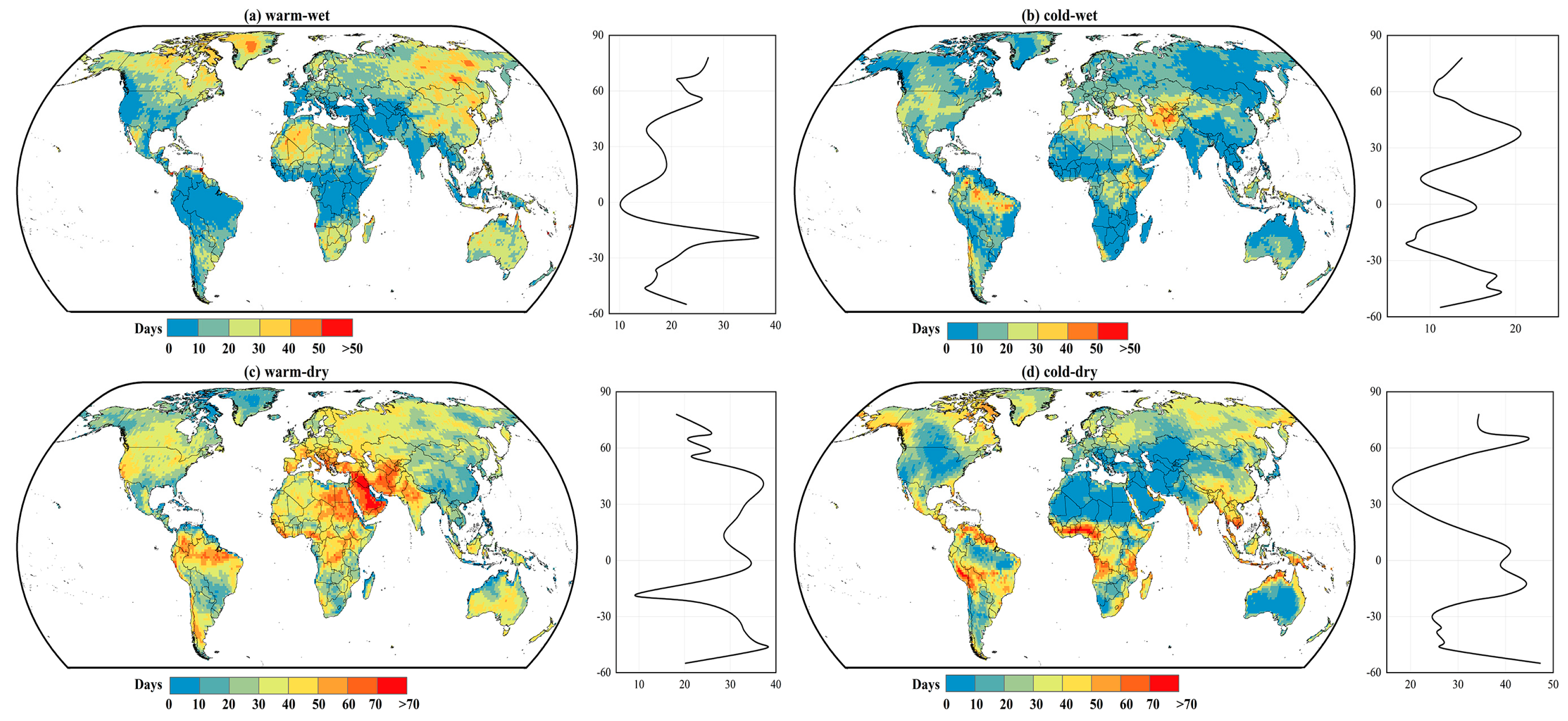
3.2. Changes in the Spatial Pattern of Compound Extreme Events

In order to study whether there is spatial aggregation of the four compound extreme climate indices, we calculated the global Moran’s I of these four events every ten years, and the results are shown in

Table 4. Change in Moran’s I of four compound indices.

		2020	2030	2040	2050	2060	2070	2080	2090	2100
warm–wet	Moran’s I	0.34	0.35	0.38	0.4	0.36	0.38	0.36	0.28	0.41
	Z	6.14	6.26	6.89	7.22	6.08	6.83	6.47	5.12	7.46
	p	0	0	0	0	0	0	0	0	0
cold–wet	Moran’s I	0.78	0.75	0.76	0.8	0.73	0.76	0.74	0.66	0.71
	Z	13.89	13.21	13.46	14.25	12.84	13.38	13.13	11.62	12.54
	p	0	0	0	0	0	0	0	0	0
warm–dry	Moran’s I	0.38	0.45	0.46	0.48	0.46	0.5	0.43	0.45	0.53
	Z	6.82	8.05	8.19	8.49	8.22	8.83	7.73	7.96	9.37
	p	0	0	0	0	0	0	0	0	0
cold–dry	Moran’s I	0.68	0.7	0.67	0.7	0.71	0.73	0.65	0.66	0.64
	Z	11.97	12.37	11.94	12.41	12.58	12.83	11.59	11.69	11.35
	p	0	0	0	0	0	0	0	0	0

. The Z-scores in different years are all higher than the critical value of 2.58 at a significance level of 0.01, which is statistically significant. This indicates that the four compound extreme climate indices exhibit a spatial positive correlation on a global scale and exhibit significant spatial clustering rather than a random distribution. The Moran’s I of the warm–wet event fluctuated in the range of about 0.3–0.4. The years of 2090 and 2100 were the years with the weakest and strongest aggregation, and the Moran’s I was 0.28 and 0.41, respectively. The Moran’s I of the cold–wet event fluctuated in the range of 0.7–0.8. The Moran’s I in 2090 and 2050 was 0.66 and 0.8, respectively. The spatial clustering of the warm–dry event shows a state of strengthening–weakening–strengthening. The spatial clustering in 2020 is the weakest, and the Moran’s I is 0.38, the strongest in 100, with a value of 0.53. The Moran’s I range of the cold–dry event is about 0.6–0.7, and the spatial agglomeration in the next 80 years will show a pattern of first strengthening, and then weakening. Its spatial agglomeration was the strongest in 2070 and the weakest in 2100, with a Moran’s I of 0.73 and 0.64, respectively.

We use hot spot analysis to intuitively experience the spatial distribution patterns of four compound extreme climate events worldwide. Figure 4 shows the hot and cold point regions of the four indices in 2060. Based on the confidence level of the calculation results, we have set three different levels for the hot spot area and the cold spot area. The hot spots of the warm–wet event occur in countries and regions such as northwestern Africa, Mongolia, North Korea, and Greenland. Its cold spots occur in the border area between West Asia and North Africa, eastern Africa, and western South America. The hot spots of the cold–wet event occur in northern and southwestern Asia, southern Europe, and northern and eastern Africa. Its cold spots are mainly distributed in eastern South America, and western and southern Africa, as well as parts of South Asia. The northern and southwestern regions of Asia, as well as parts of northern Africa and southern Europe, are hot spots for the warm–dry event, while the United States and parts of North America are cold spots. Overall, the spatial distribution of cold spots and hot spots of the cold–dry event is the opposite of that in the cold–wet event, with some differences in southern Africa.

Similarly, we used the hot spot analysis method to analyze the spatial distribution patterns of four extreme indices in 2100 (Figure 5). The hot spots where the warm–wet event occur are located in North Asia, and northwestern and southern Africa, while cold spots occur in southwestern Asia, eastern Africa, and western South America. The hot spots of the cold–wet event occur in West Asia, northeastern Africa, and southern Europe, while the cold spots occur in South Asia, and southern and eastern Africa. West Asia, southern Europe, and northeastern Africa are hot spots for the warm–dry event, with almost no cold spots except for a small portion of South Asia and the Americas. The hot spots of the cold–dry event are distributed in eastern South America, South Asia, and parts of western Africa, while the cold spots are concentrated in western Asia, northern Africa, and southern Europe. Compared with 2060, we find that, in 2000, the area of hot spots and cold spots of the warm–wet event will increase, while the area of hot spots and cold spots of the other three compound extreme weather events will decrease.

Through the hot spot analysis and cold spot analysis, we can intuitively see the high-value and low-value regions of the four compound extreme weather events in space. In order to further study the spatial distribution of the four extreme weather events, we calculated the spatial distribution of different indices and the changes in different latitudes. Figure 6 shows the spatial distribution of the four indices in 2060 and the changes in the average values of the indices at different latitudes. The high-value areas of the warm–wet event are located in high-latitude regions, such as North Asia and Greenland. In the southern hemisphere, the high-value areas of this event include regions such as Australia, which can last up to 40–50 days. In West Asia, central Africa, and northern South America, the low-value areas of this event occur within 10 days per year. The high values of the number of days during which the cold–wet event occurs are the opposite of that of the warm–wet event, which are distributed in parts of West Asia, North Africa, southern Europe, and northern South America. The distribution rule of the average value of the days of two events along the latitude is basically the opposite. There is a significant difference in the global spatial distribution of the number of days of the warm–dry event and the cold–dry event, with high-value regions reaching around 80 days, while low-value regions have less than 10 days. The high-value areas of the warm–dry event are concentrated in West Asia and North Africa, while the high-value areas of the cold–dry event are mainly distributed in South Asia, southern Africa, and central and western South America.

Figure 7 shows the spatial distribution of the occurrence days of four compound extreme climate events in 2100. In 2100, the global spatial distribution pattern of the four indices will basically be consistent with that of 2060, with slight changes in intensity. For the warm–wet event, the number of days in the latitude near the Tropic of Capricorn increased significantly by about 10 days, and the equator is still the area with the least number of days for the event, which is about 10 days. For the cold–dry event, the differences are mainly reflected in regions above a 60 degrees north latitude. In 2100, starting from a 60 degrees north latitude, the higher the latitude, the more days the event occurred, while, in 2060, the opposite conclusion was reached. Compared with 2060, the number of warm–dry events in 2100 in latitudes above the Arctic Circle will increase, while the number of days in a 50–60 degrees south latitude will decrease. The difference in the cold–dry event is mainly reflected around a 60 degrees south latitude, with an increase in the number of days this event occurred in 2100 compared to 2060.

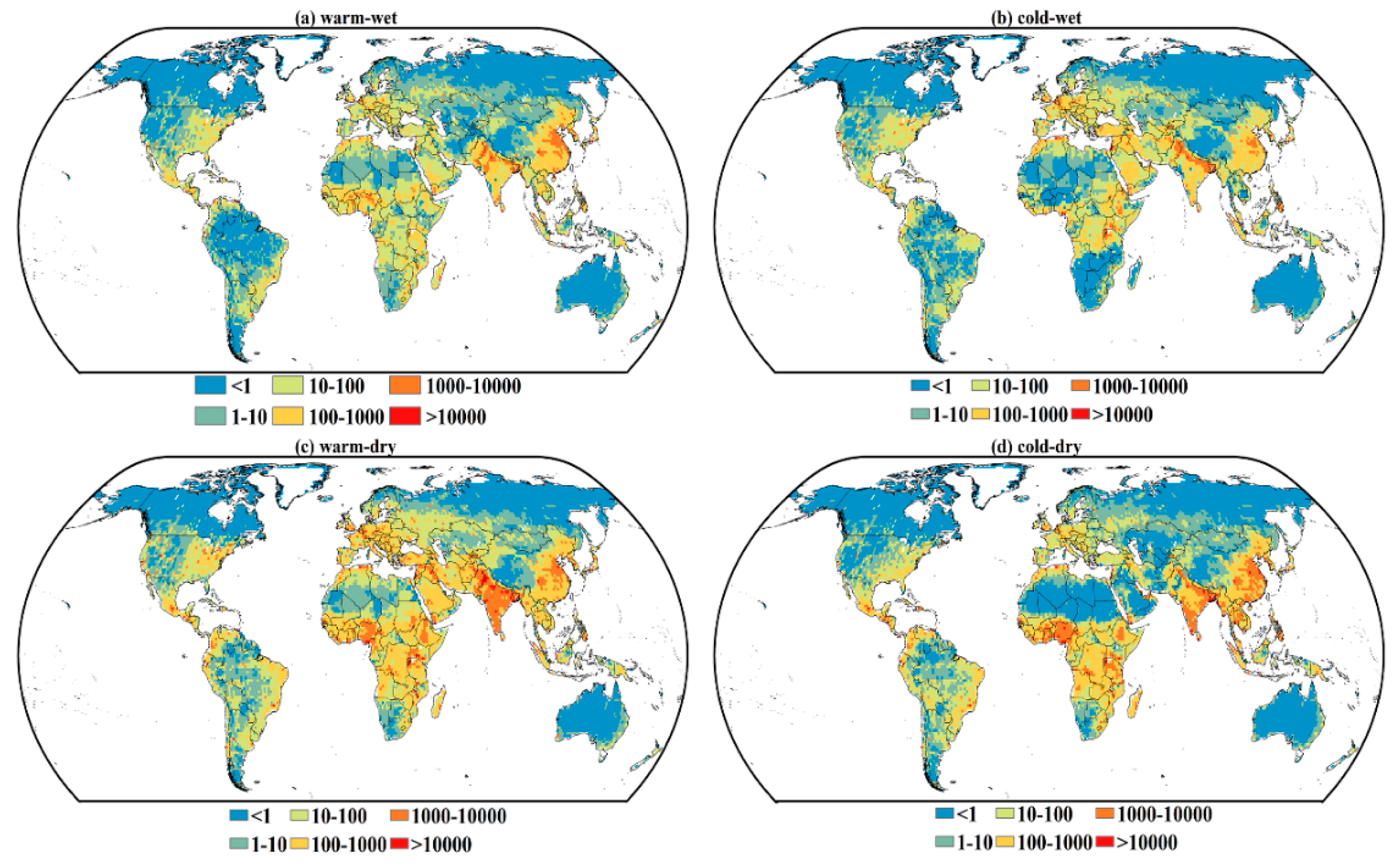
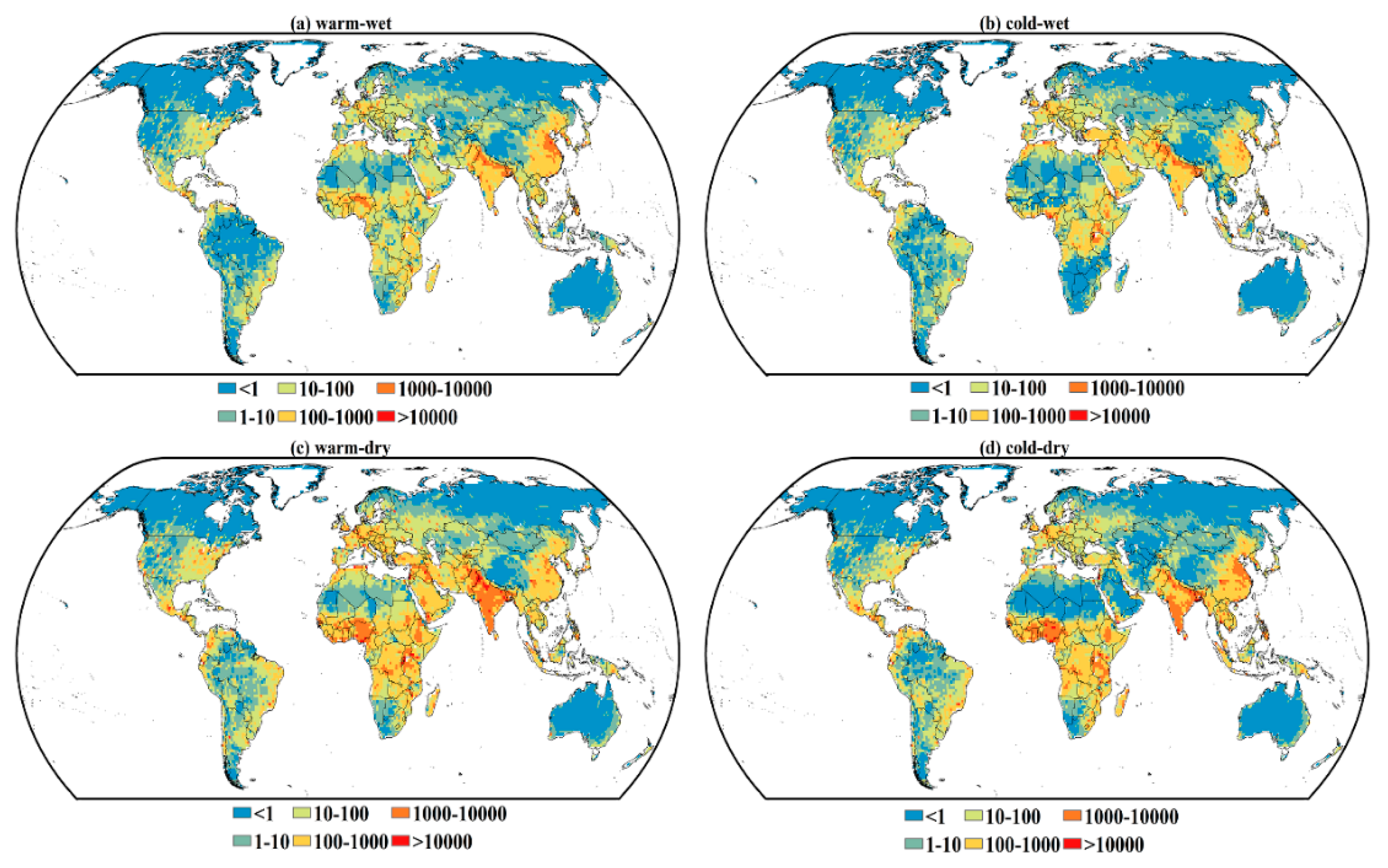
3.3. The Spatial Distribution of Population Exposure under Different Compound Extreme Events

We calculated the population exposure under different extreme indices. In order to intuitively perceive the exposure of the global population under different composite events, we divided the exposure levels into six levels: extremely low (less than 10³ person · day), low (10³–10⁴ person · day), relatively low (10⁴–10⁵ person · day), medium (10⁵–10⁶ person · day), high (10⁶–10⁷ person · day), and extremely high (exceed 10⁷ person · day). Figure 8 shows the population exposure under different climate events in 2060. For warm–wet events and cold–wet events, areas with a medium-level exposure or higher are mainly distributed in East Asia, South Asia, central and western Asia, central Africa, and western Europe. Areas where people have exposure levels of medium or higher under two extreme events accounted for 12.75% and 13.16% of the total land area, respectively. For the warm–dry event and cold–dry event, regions with medium or higher exposure levels are mainly distributed in East Asia, Southeast Asia, South Asia, central Asia, West Asia, central Africa, and western Europe. Areas with a medium or higher population exposure account for 23.54% and 18.83% of the total land area, respectively. East Asia and South Asia are the regions with the highest population density in the world. According to the exposure calculation formula, it is not difficult to see that these two regions are also the areas with the highest population exposure. Increasing the area of public green space, improving the health and medical security of residents, is particularly important for reducing the harm of extreme weather events to local residents.

Figure 9 shows the exposure of the population to four compound extreme events in 2100. Their spatial distribution is basically consistent with the pattern in 2060. The difference is that the proportion of areas with a population exposure level of medium or higher has increased. The proportion of areas corresponding to warm–wet, cold–wet, warm–dry, and cold–dry events is 13.07%, 13.49%, 25.17%, and 19.21%, respectively. Obviously, when we focus on exposure levels of medium or higher, the proportion of compound events related to dry conditions is larger than that related to wet conditions. It can also be said that extreme events related to drought have a greater impact on humans. Under the four extreme events, we can also see that the population exposure levels in East Asia, South Asia (mainly in India), and central Africa are higher than those in other regions. These areas are also areas that urgently need to strengthen extreme climate monitoring and risk prevention.

4. Discussion

We find that there were significant changes in events related to humidity. From the results of the M-K mutation test, it can be seen that events related to drought will change in a more complex manner in the next 80 years, and the corresponding UF and UB curves have multiple intersections, which also means that events related to drought are complex and variable. As we all know, the year when a certain climate event suddenly changes is the year when climate disasters are most likely to occur, so we should be vigilant against drought disasters in the future. From a spatial perspective, the number of days that compound events related to drought occur varies greatly worldwide. Compound warm–dry events occur for less than 10 days per year in high latitude areas such as Greenland, while the maximum number of days per year can reach over 80 days in regions such as West Asia and South Asia. Zhang has found the spatial distribution of global drought, which is basically consistent with our conclusion, indicating that Africa is a relatively arid region [45]. There are also studies predicting future climate change, indicating that the increase in compound extreme heat events in low-latitude regions is more prominent than in mid-latitude regions [46]. Hao’s research found that, under the background of global warming, the probability of extreme events with a combined high temperature and drought has increased [47]. The existing research shows that the predicted high temperature and drought complex extreme events in northern Eurasia, Europe, Southeast Australia, most regions of the United States, and India will increase, and these regions will face a greater risk of high temperature and drought complex extreme events in the future [48,49]. In the future, these regions will face a greater risk of combined extreme events of high temperature and drought.

It should be noted that, from the mid-20th century to the late 20th century, under four compound events, the area with a population exposure level of intermediate or higher will increase. It is worth noting that East Asia, South Asia, and central Africa need to develop corresponding policies to protect sensitive populations such as the elderly and children, as these regions have a high population density and lower resistance to climate risks. Faced with the increasingly severe impact of extreme events, countries around the world must quickly prepare for disaster prevention and reduction, and strengthen adaptation actions. When formulating extreme event prevention plans and countermeasures, it is necessary to adapt to local conditions and consider the climate characteristics of the local and surrounding areas. In addition, it is necessary to increase the construction of extreme event monitoring and warning systems, and strengthen the monitoring and warning of extreme events and their risks. The study of compound extreme events involves a wide range of fields, and the multiple factors themselves can belong to different weather and climate variables, as well as a combination of driving and disaster-causing factors. Scholars have used neural network methods or established risk assessment systems to evaluate the environmental risk levels of residents in different regions [50,51]. Therefore, more interdisciplinary, cross-departmental, and cross-regional research is needed in the future.

There are certain limitations and uncertainties in this paper. The accuracy of the prediction results is related to the accuracy of the model used. For the five data sources, we used a simple arithmetic mean method to obtain the values of climate factors. Although it can reduce some errors, it is best to compare it with other bias correction methods in future research. In addition, we used the SSP2-4.5 scenario (moderate-compulsion scenario) for prediction, and, if the low-compulsion scenario and the high-compulsion scenario, such as the SSP1-2.6 scenario and the SSP5-8.5 scenario, are used, different results may be obtained. The use of data from different future scenarios in local areas for prediction is also a direction for future efforts.

5. Conclusions

This study estimates the temporal and spatial patterns of four compound extreme climate events (including warm–dry, warm–wet, cold–dry and cold–wet) and the corresponding population exposure based on CMIP6 models. The following conclusions can be drawn from this study:

(1)

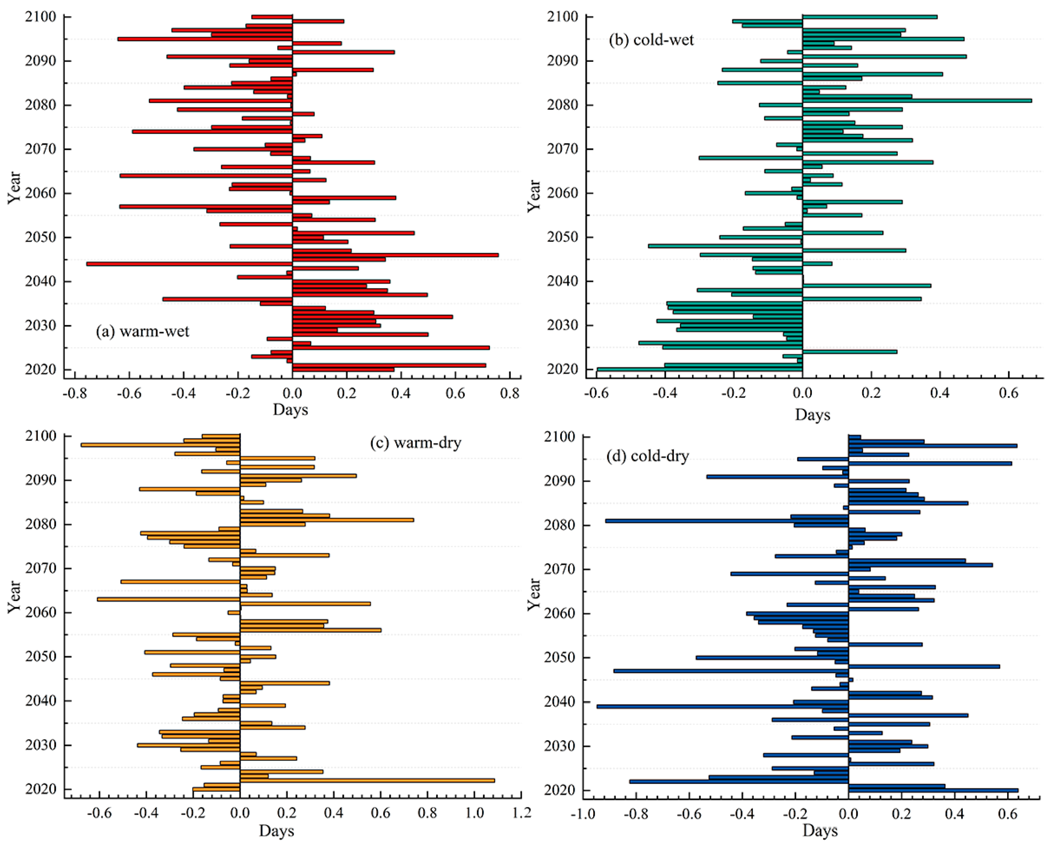
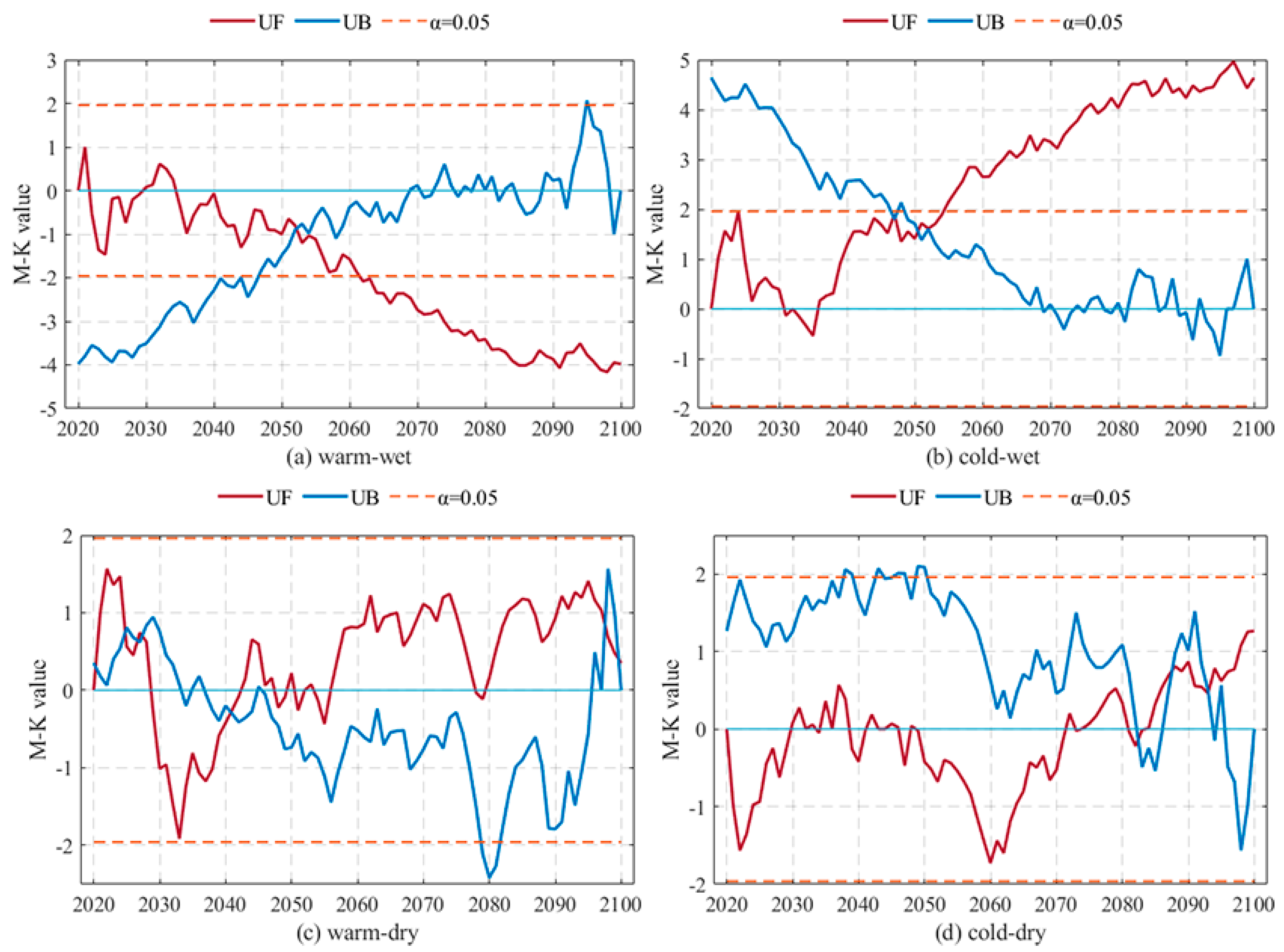
In the future period from 2020 to 2100, there will be a significant downward trend in the warm–wet event, with a decline rate of 0.06 days per decade. Cold–wet events show a significant increasing trend, with an increase rate of 0.06 days per decade. Warm–dry events and cold–dry events show an upward trend, with rates of 0.01 days per decade and 0.02 days per decade, respectively.

(2)

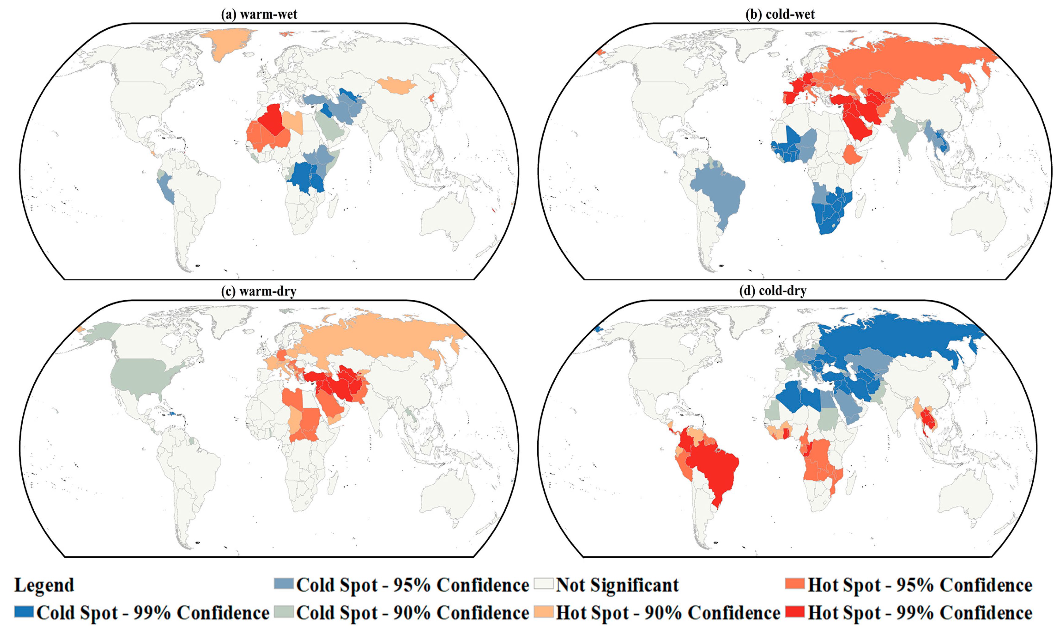
West Asia is a hot area where warm–dry events and cold–wet events occur. Northern Africa is a high-risk area for the warm–wet event, while countries such as Brazil in South America are hot spots for the cold–dry event. To address climate risks, regional exchanges and co-operation are necessary.

(3)

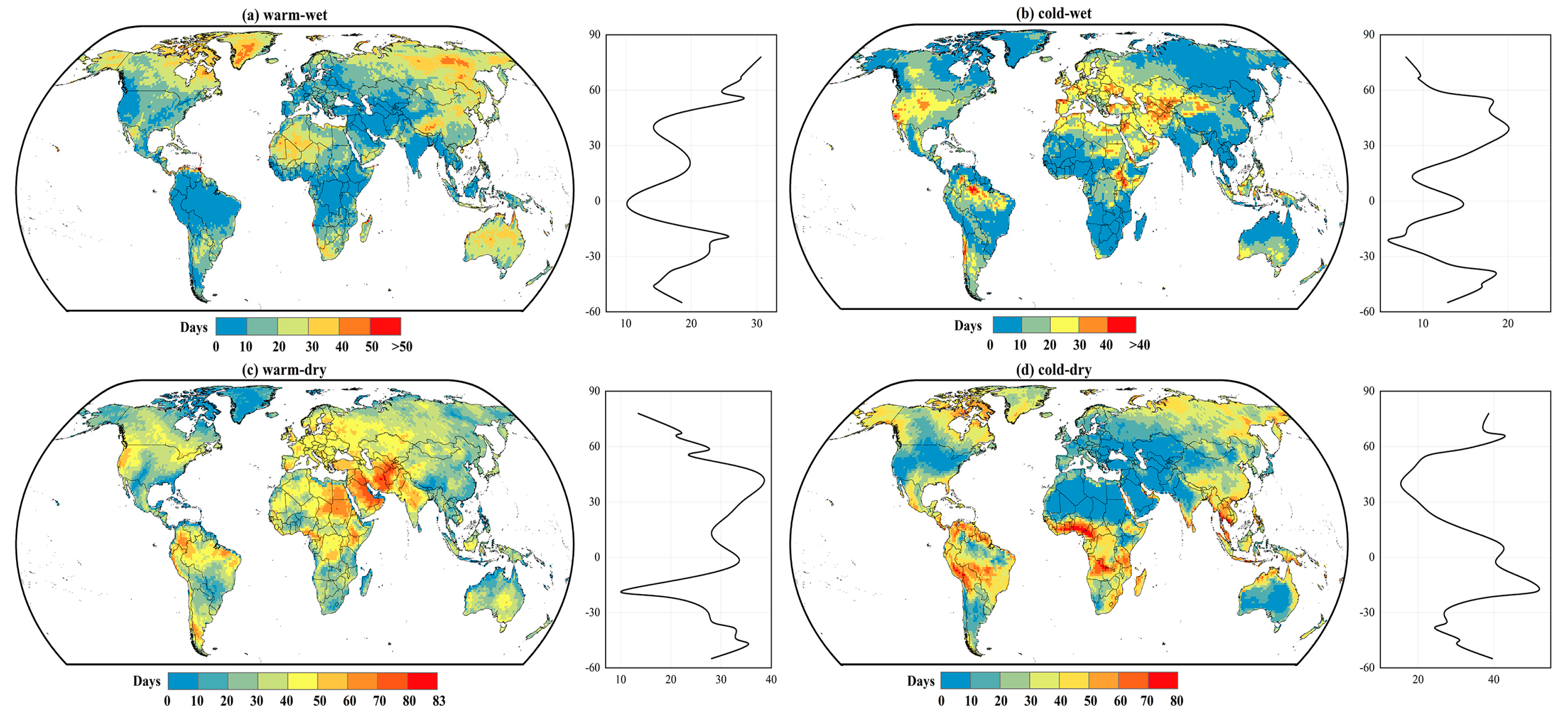
The intensity of the warm–wet event in the southern hemisphere is higher than that in the northern hemisphere, and the area with the highest number of warm and humid event days is located near a 20 degrees south latitude. The intensity of the cold–wet event is higher in the northern hemisphere than in the southern hemisphere. The intensity of the warm–dry event in the northern hemisphere is higher than that in the southern hemisphere. The intensity of the cold–dry event is strongest near a 60 degrees north and south latitude.

(4)

East Asia, South Asia, and central Africa have higher levels of population exposure globally than other regions. Areas with medium (10⁵ person · day) or higher population exposure levels for warm–wet and cold–wet events both account for approximately 13% of the total area, while warm–dry and cold- dry events account for 25% and 19% of the total area, respectively.

References

1. Mazdiyasni, O.; AghaKouchak, A.; Davis, S.J.; Madadgar, S.; Mehran, A.; Ragno, E.; Sadegh, M.; Sengupta, A.; Ghosh, S.; Dhanya, C.T.; et al. Increasing probability of mortality during Indian heat waves. Sci. Adv. 2017, 3, e1700066. [Google Scholar] [CrossRef] [PubMed]
2. Gu, X.; Zhang, Q.; Li, J.; Singh, V.P.; Liu, J.; Sun, P.; Cheng, C. Attribution of global soil moisture drying to human activities: A quantitative viewpoint. Geophys. Res. Lett. 2019, 46, 2573–2582. [Google Scholar] [CrossRef]
3. Satoh, Y.; Yoshimura, K.; Pokhrel, Y.; Kim, H.; Shiogama, H.; Yokohata, T.; Hanasaki, N.; Wada, Y.; Burek, P.; Byers, E.; et al. The timing of unprecedented hydrological drought under climate change. Nat. Commun. 2022, 13, 3287. [Google Scholar] [CrossRef]
4. Li, C.; Gu, X.; Slater, L.J.; Liu, J.; Li, J.; Zhang, X.; Kong, D. Urbanization-Induced Increases in Heavy Precipitation are Magnified by Moist Heatwaves in an Urban Agglomeration of East China. J. Clim. 2023, 36, 693–709. [Google Scholar] [CrossRef]
5. Fouillet, A.; Rey, G.; Laurent, F.; Pavillon, G. Excess mortality related to the August 2003 heat wave in France. Int. Arch. Occup. Environ. Health 2006, 80, 16–24. [Google Scholar] [CrossRef] [PubMed]
6. Sun, X.; Sun, Q.; Zhou, X.; Li, X.; Yang, M.; Yu, A.; Geng, F. Heat wave impact on mortality in Pudong New Area, China in 2013. Sci. Total Environ. 2014, 493, 789–794. [Google Scholar] [CrossRef] [PubMed]
7. Van Oldenborgh, G. Rapid Attribution of the Extreme Rainfall in Texas from Tropical Storm Imelda. 2019. Available online: https://www.worldweatherattribution.org/rapid-attribution-of-the-extreme-rainfall-in-texas-from-tropical-storm-imelda/ (accessed on 1 September 2023).
8. Ridder, N.; Pitman, A.; Westra, S.; Ukkola, A.; Hong, X.; Bador, M.; Hirsch, A.L.; Evans, J.; Di Luca, A.; Zscheischler, J. Global hotspots for the occurrence of compound events. Nat. Commun. 2020, 11, 5956. [Google Scholar] [CrossRef] [PubMed]
9. Zhang, P.; Jeong, J.-H.; Yoon, J.-H.; Kim, H.; Wang, S.; Linderholm, H.W.; Fang, K.; Wu, X.; Chen, D. Abrupt shift to hotter and drier climate over inner East Asia beyond the tipping point. Science 2020, 370, 1095–1099. [Google Scholar] [CrossRef]
10. Guan, Y.; Gu, X.; Slater, L.; Li, L.; Kong, D.; Liu, J.; Zhang, X.; Yan, X. Tracing anomalies in moisture recycling and transport to two record-breaking droughts over the Mid-to-Lower Reaches of the Yangtze River. J. Hydrol. 2022, 609, 127787. [Google Scholar] [CrossRef]
11. Yu, X.; Gu, X.; Kong, D.; Zhang, Q.; Cao, Q.; Slater, L.J.; Ren, G.; Luo, M.; Li, J.; Liu, J.; et al. Asymmetrical shift toward less light and more heavy precipitation in an urban agglomeration of East China: Intensification by urbanization. Geophys. Res. Lett. 2022, 49, e2021GL097046. [Google Scholar] [CrossRef]
12. Zscheischler, J.; Seneviratne, S.I. Dependence of drivers affects risks associated with compound events. Sci. Adv. 2017, 3, e1700263. [Google Scholar] [CrossRef] [PubMed]
13. Sarhadi, A.; Ausín, M.C.; Wiper, M.P.; Touma, D.; Diffenbaugh, N.S. Multidimensional risk in a nonstationary climate: Joint probability of increasingly severe warm and dry conditions. Sci. Adv. 2018, 4, aau3487. [Google Scholar] [CrossRef]
14. Willett, K.M.; Sherwood, S. Exceedance of heat index thresholds for 15 regions under a warming climate using the Wet-Bulb Globe temperature. Int. J. Climatol. 2012, 32, 161–177. [Google Scholar] [CrossRef]
15. Schwingshackl, C.; Sillmann, J.; Vicedo-Cabrera, A.M.; Sandstad, M.; Aunan, K. Heat stress indicators in CMIP6: Estimating future trends and exceedances of impact-relevant thresholds. Earths Future 2021, 9, e2020EF001885. [Google Scholar] [CrossRef]
16. Barriopedro, D.; Fischer, E.M.; Luterbacher, J.; Trigo, R.M.; GarcíaHerrera, R. The hot summer of 2010: Redrawing the temperature record map of Europe. Science 2011, 332, 220–224. [Google Scholar] [CrossRef]
17. Grumm, R.H. The central European and Russian heat event of July–August 2010. Bull. Am. Meteorol. 2011, 92, 1285–1296. [Google Scholar] [CrossRef]
18. Witte, J.C.; Douglass, A.R.; da Silva, A.; Torres, O.; Levy, R.; Duncan, B.N. NASA A-Train and Terra observations of the 2010 Russian wildfires. Atmos. Chem. Phys. 2011, 11, 9287–9301. [Google Scholar] [CrossRef]
19. Hauser, M.; Orth, R.; Seneviratne, S.I. Role of soil moisture versus recent climate change for the 2010 heat wave in western Russia. Geophys. Res. Lett. 2016, 43, 2819–2826. [Google Scholar] [CrossRef]
20. IPCC. Summary for Policymakers, Climate Change 2021: The Physical Science Basis; Cambridge University Press: Cambridge, UK, 2021; pp. 3–32. [Google Scholar]
21. Wu, X.; Hao, Z.; Hao, F.; Zhang, X. Variations of compound precipitation and temperature extremes in China during 1961–2014. Sci. Total Environ. 2019, 663, 731–737. [Google Scholar] [CrossRef]
22. Ciais, P.; Reichstein, M.; Viovy, N.; Granier, A.; Ogée, J.; Allard, V.; Aubinet, M.; Buchmann, N.; Bernhofer, C.; Carrara, A.; et al. Europe-wide reduction in primary productivity caused by the heat and drought in 2003. Nature 2005, 437, 529–533. [Google Scholar] [CrossRef]
23. Allen, C.D.; Macalady, A.K.; Chenchouni, H.; Bachelet, D.; McDowell, N.; Vennetier, M.; Kitzberger, T.; Rigling, A.; Breshears, D.D.; Hogg, E.H.; et al. A global overview of drought and heat-induced tree mortality reveals emerging climate change risks for forests. For. Ecol. Manag. 2010, 259, 660–684. [Google Scholar] [CrossRef]
24. Bandyopadhyay, S.; Kanji, S.; Wang, L. The impact of rainfall and temperature variation on diarrheal prevalence in sub-Saharan Africa. Appl. Geogr. 2012, 33, 63–72. [Google Scholar] [CrossRef]
25. Schmidli, J.; Frei, C. Trends of heavy precipitation and wet and dry spells in Switzerland during the 20th century. Int. J. Climatol. 2005, 25, 753–771. [Google Scholar] [CrossRef]
26. Benestad, R.E.; Haugen, J.E. On complex extremes: Flood hazards and combined high spring-time precipitation and temperature in Norway. Clim. Chang. 2007, 85, 381–406. [Google Scholar] [CrossRef]
27. Eyring, V.; Bony, S.; Meehl, G.A.; Senior, C.A.; Stevens, B.; Stouffer, R.J.; Taylor, K.E. Overview of the coupled model intercomparison project phase 6 (CMIP6) experimental design and organization. Geosci. Model Dev. 2016, 9, 1937–1958. [Google Scholar] [CrossRef]
28. Stouffer, R.J.; Eyring, V.; Meehl, G.A.; Bony, S.; Senior, C.; Stevens, B.; Taylor, K.E. CMIP5 scientific gaps and recommendations for CMIP6. Bull. Am. Meteorol. 2017, 98, 95–105. [Google Scholar] [CrossRef]
29. Rohat, G.; Flacke, J.; Dosio, A.; Dao, H.; van Maarseveen, M. Projections of human exposure to dangerous heat in African cities under multiple socioeconomic and climate scenarios. Earths Future 2019, 7, 528–546. [Google Scholar] [CrossRef]
30. Riahi, K.; van Vuuren, D.P.; Kriegler, E.; Edmonds, J.; O’Neill, B.C.; Fujimori, S.; Bauer, N.; Calvin, K.; Dellink, R.; Fricko, O.; et al. The shared socioeconomic pathways and their energy, land use, and greenhouse gas emissions implications: An overview. Glob. Environ. Chang. 2017, 42, 153–168. [Google Scholar] [CrossRef]
31. Beniston, M. Trends in joint quantiles of temperature and precipitation in Europe since 1901 and projected for 2100. Geophys. Res. Lett. 2009, 36, L07707. [Google Scholar] [CrossRef]
32. Hao, Z.; AghaKouchak, A.; Phillips, T.J. Changes in concurrent monthly precipitation and temperature extremes. Environ. Res. Lett. 2013, 8, 034014. [Google Scholar] [CrossRef]
33. Yue, S.; Pilon, P.; Cavadias, G. Power of the Mann-Kendall and Spearman’s rho tests for detecting monotonic trends in hydrological series. J. Hydrol. 2002, 259, 254–271. [Google Scholar] [CrossRef]
34. Gocic, M.; Trajkovic, S. Analysis of changes in meteorological variables using Mann–Kendall and Sen’s slope estimator statistical tests in Serbia. Glob. Planet Chang. 2013, 100, 172–182. [Google Scholar] [CrossRef]
35. Mann, H. Nonparametric test against trend. Econometrica 1945, 13, 245–259. [Google Scholar] [CrossRef]
36. Kendall, M. Rank Correlation Methods. 1948. Available online: https://psycnet.apa.org/record/1948-15040-000 (accessed on 11 September 2023).
37. Thompson, E.; Saveyn, P.; Declercq, M.; Meert, J.; Guida, V.; Eads, C.D.; Robles, E.S.J.; Britton, M.M. Characterisation of heterogeneity and spatial autocorrelation in phase separating mixtures using Moran’s I. J. Colloid Interface Sci. 2018, 513, 180–187. [Google Scholar] [CrossRef] [PubMed]
38. Zhang, T.; Lin, G. On Moran’s I coefficient under heterogeneity. Comput. Stat. Data Ann. 2016, 95, 83–94. [Google Scholar] [CrossRef]
39. Cliff, A.D.; Ord, J.K. Spatial Processes: Models and Applications; Pion Limited: London, UK, 1981. [Google Scholar]
40. Getis, A.; Ord, J.K. The analysis of spatial association by use of distance statistics. Geogr. Anal. 1992, 24, 189–206. [Google Scholar] [CrossRef]
41. Streletskiy, D.A.; Sherstiukov, A.B.; Frauenfeld, O.W.; Nelson, F.E. Changes in the 1963–2013 shallow ground thermal regime in Russian permafrost regions. Environ. Res. Lett. 2015, 10, 125005. [Google Scholar] [CrossRef]
42. Liu, D.; Zhao, Q.; Guo, S.; Liu, P.; Xiong, L.; Yu, X.; Zou, H.; Zeng, Y.; Wang, Z. Variability of spatial patterns of autocorrelation and heterogeneity embedded in precipitation. Hydrol. Res. 2019, 50, 215–230. [Google Scholar] [CrossRef]
43. Jones, B.; O’Neill, B.C.; McDaniel, L. Future population exposure to US heat extremes. Nat. Clim. Chang. 2015, 5, 652–655. [Google Scholar] [CrossRef]
44. Jones, B.; O’Neill, B.C. Spatially explicit global population scenarios consistent with the Shared Socioeconomic Pathways. Environ. Res. Lett. 2016, 11, 084003. [Google Scholar] [CrossRef]
45. Zhang, G.; Wang, H.; Gan, T.; Zhang, S.; Shi, L.; Zhao, J.; Su, X.; Song, S. Climate Change Determines Future Population Exposure to Summertime Compound Dry and Hot Events. Earths Future 2022, 10, e2022EF003015. [Google Scholar] [CrossRef]
46. Li, D.; Yuan, J.; Kopp, R.E. Escalating global exposure to compound heat-humidity extremes with warming. Environ. Res. Lett. 2020, 15, 064003. [Google Scholar] [CrossRef]
47. Hao, Z.; Hao, F.; Singh, V.P.; Zhang, X. Changes in the severity of compound drought and hot extremes over global land areas. Environ. Res. Lett. 2018, 13, 124022. [Google Scholar] [CrossRef]
48. Herrera-Estrada, J.E.; Sheffield, J. Uncertainties in future projections of summer droughts and heat waves over the contiguous United States. J. Clim. 2017, 30, 6225–6246. [Google Scholar] [CrossRef]
49. Schubert, S.D.; Wang, H.; Koster, R.D.; Suarez, M.J.; Groisman, P.Y. Northern Eurasian heat waves and droughts. J. Clim. 2014, 27, 3169–3207. [Google Scholar] [CrossRef]
50. Pietrucha, K.; Tchórzewska, B. Water Supply System operation regarding consumer safety using Kohonen neural network. In Safety, Reliability and Risk Analysis: Beyond the Horizon; CRC Press: Boca Raton, FL, USA, 2014; pp. 1115–1120. [Google Scholar]
51. Janusz, R.; Barbara, T.; Katarzyna, P. A Hazard Assessment Method for Waterworks Systems Operating in Self-Government Units. Int. J. Environ. Res. Public Health 2019, 16, 767. [Google Scholar] [CrossRef]
Figure 1. Changes in four compound extreme indices from 2020 to 2100.
Sustainability 16 05007 g001
Figure 2. Changes in the anomalies of four compound extreme indices from 2020 to 2100.
Sustainability 16 05007 g002
Figure 3. M-K mutation test results for four composite indices.
Sustainability 16 05007 g003
Figure 4. Hot spot analysis of four compound indices in 2060.
Sustainability 16 05007 g004
Figure 5. Hot spot analysis of four compound indices in 2100.
Sustainability 16 05007 g005
Figure 6. The spatial distribution of four compound indices in 2060.
Sustainability 16 05007 g006
Figure 7. The spatial distribution of four compound indices in 2100.
Sustainability 16 05007 g007
Figure 8. Spatial distribution of the global population exposure to compound indices in 2060 (Unit: 103 person · day).
Sustainability 16 05007 g008
Figure 9. Spatial distribution of the global population exposure to compound indices in 2100 (Unit: 103 person · day).
Sustainability 16 05007 g009