From Individual Motivation to Geospatial Epidemiology: A Novel Approach Using Fuzzy Cognitive Maps and Agent-Based Modeling for Large-Scale Disease Spread

Abstract

In the past few years, there have been many studies addressing the simulation of COVID-19’s spatial transmission model of infectious disease in time. However, very few studies have focused on the effect of the epidemic environment variables in which an individual lives on the individual’s behavioral logic leading to changes in the overall epidemic transmission trend at larger scales. In this study, we applied Fuzzy Cognitive Maps (FCMs) to modeling individual behavioral logistics, combined with Agent-Based Modeling (ABM) to perform “Susceptible—Exposed—Infectious—Removed” (SEIR) simulation of the independent individual behavior affecting the overall trend change. Our objective was to simulate the spatiotemporal spread of diseases using the Bengaluru Urban District, India as a case study. The results show that the simulation results are highly consistent with the observed reality, in terms of trends, with a Root Mean Square Error (RMSE) value of 0.39. Notably, our approach reveals a subtle link between individual motivation and infection-recovery dynamics, highlighting how individual behavior can significantly impact broader patterns of transmission. These insights have potential implications for epidemiologic strategies and public health interventions, providing data-driven insights into behavioral impacts on epidemic spread. By integrating behavioral modeling with epidemic simulation, our study underscores the importance of considering individual and collective behavior in designing sustainable public health policies and interventions.

1. Introduction

By the end of 2023, more than 773 million cumulative cases of COVID-19 and over 6 million deaths had been reported worldwide [1]. Contrary to the exponential pattern spread of previous pandemics in early stages, such as H1N1 in 2009 [2] or the 2014 Ebola outbreak in West Africa [3], there was a sub-exponential increase in confirmed cases in many parts of the globe [4], rather than the expected exponential increase (typical of an unconfined outbreak). This was due to a combination of rapid and effective public health interventions, extensive quarantine policies, and changes in public behavior that significantly slowed the spread of the virus. The unparalleled scope and intensity of COVID-19’s spread and heightened governmental and public attentiveness set it apart from earlier infectious diseases. The worldwide concern over COVID-19 prompted diverse intervention measures by governments and varied daily self-protection behavior by individuals. These complexities have rendered the simulation of COVID-19’s spreading pattern more intricate than its predecessors.

Ever since Kermack and McKendrick (1927) [5] proposed the “Susceptible—Infectious—Removed” (SIR) model for simulation of infectious disease simulation studies, the SIR model and its variants have been widely used as an effective mathematical model for describing the transmission process of a particular infectious disease in a population. Depending on the characteristics of the infectious disease under study, its variant, the “Susceptible—Infectious—Susceptible” (SIS) model [6,7] is applied to diseases that do not acquire long-term immunity, while the “Susceptible—Exposed—Infectious—Removed” (SEIR) model [8,9] is more suitable for diseases with an incubation period. In recent decades, the advent of computational methodologies has revolutionized the modeling of intricate systems, especially in the realm of epidemiology [10]. Fuzzy Cognitive Maps (FCMs) have often been used in epidemiological research to address challenges related to spatial decision making [11]. Introduced by Kosko (1986) [12], FCMs capture the essence of systems by translating qualitative data into a quantifiable form. Fuzzy Cognitive Maps, structured as signed directed graphs, allow the establishment of causal relationships between system concepts, thereby providing an insightful representation of dynamics, especially in contexts imbued with uncertainty and imprecision. Parallel to the development of FCMs, Agent-Based Modeling (ABM) emerged as a pivotal tool. Rooted in its ability to simulate individual agents’ actions and interactions within specified environments, ABM, as delineated by Bonabeau (2002) [13], paved the way for understanding emergent phenomena in multifaceted systems. The granularity of ABM proves indispensable when melded with compartmental models like the SEIR model [14]. The ability of FCMs to represent loops and uncertainty in human decision making helps create richer agents in ABM, while the ability to simulate dynamics through space and time adds useful dimensions with which to hone FCMs [15].

Notably, combining ABM with SEIR introduces a granular perspective, allowing researchers to replicate individual-level interactions and behavior, thereby achieving a synthesis that reflects both micro-level intricacies and macro-level patterns in disease propagation. The pursuit of understanding infectious disease spread, exemplified by the COVID-19 pandemic, has led to a myriad of modeling approaches to predicting and mitigating potential outbreaks. Several foundational studies in recent years have delineated crucial aspects of these methodologies, which our current research both builds upon and diverges from in essential ways. For example, Chen et al., (2020) [16] developed a Bat-Host-Reservoir–People transmission network, which illuminated the initial transmission dynamics of COVID-19, particularly underscoring a significant finding: the basic reproductive number (R0) from nature-to-human transmission was considerably less potent than human-to-human transmission. Such insight provides a nuanced perspective on the initial stages of zoonotic outbreaks, emphasizing the transition from animal-to-human transmission to subsequent human interactions. Li et al., (2020) [17] reverse-engineered statistical data to pinpoint the R0 during the infancy of human-to-human transmission. The results offer a tangible representation of the virus’s contagiousness, forming an empirical foundation that can be compared against various modeling outputs. Subsequent research then shifted focus to policy implications, dissecting the temporal impacts of Non-Pharmaceutical Interventions (NPIs) in the UK and the US. Such studies, by parsing out the short-term R0 fluctuations post the implementation or cessation of NPIs, render valuable policy directives. Lyu et al., (2021) [18] proposed a method using spatiotemporal kernel density estimation (STKDE) to explore spatiotemporal clustering of high mortality rates in the United States COVID-19 centered in urban areas. They concluded that this concentration of high mortality was highly correlated with ethnicity and economic status. Expanding the geographical purview beyond COVID-19, Perez and Dragićević (2009) [19] delved into the dynamics of measles cases in Vancouver, Canada. By infusing population mobility factors, their work unveiled the spatial heterogeneity in epidemic spread, underlining the pivotal role of population movements in influencing disease trajectories. Bian (2004) [20] further enhanced this spatial perspective by offering a comprehensive approach where population segments were employed as agent groups within the SEIR framework. Leveraging interactions between adjacent areas, the authors propounded a mathematical model catering to long-distance transmissions.

Traditional epidemiological models, while valuable, often fail to capture the critical aspect of individual behavioral heterogeneity that evolves over time and space as epidemics spread. This limitation can lead to models that do not accurately reflect individual behavior and decision-making processes, thereby reducing the accuracy of infectious disease predictions and the effectiveness of assessments of the sustainability of public health security. Our research addresses this gap by integrating Fuzzy Cognitive Maps (FCMs) with Agent-Based Modeling (ABM). FCMs simulate the thinking processes of individual entities in an intuitive and transparent way, and they ensure the dynamic $R0$ value during simulation. Each individual modeled by an FCM will play an independent agent in ABM. ABM integrates factors such as population mobility, influence from neighborhood regions, and NPI policies to heighten prediction accuracy. By combining FCM and ABM, we can model how these entities interact and affect each other, thus capturing the impact of individual heterogeneity on the overall epidemic dynamics across a broader range of simulations [21]. The innovation of this hybrid approach lies in its ability to dynamically model the impact of individual behavioral logic from different communities on the overall environment, considering both local and global changes during an epidemic. This approach addresses the previous lack of spatiotemporal heterogeneity in modeling individual behavior and explores the complexity of individual motivations during epidemics. By providing a comprehensive and realistic model of disease transmission dynamics, this pioneering approach offers valuable insights for designing sustainable public health strategies and interventions. It underscores the importance of adaptive and responsive measures that can enhance the resilience and sustainability of health systems in managing epidemics.

2. Background Theory

2.1. FCM

Fuzzy Cognitive Maps (FCMs) by Kosko (1986) [12] offer a robust framework for simulating the complex interplay of individual cognition and emotions during the spread of infectious diseases. FCMs are graph-based models where nodes represent concepts (e.g., awareness of disease, fear, preventive measures) and edges denote the causal relationships between these concepts. Each edge is assigned a weight, indicating the strength and direction of the influence. FCMs describe the behavior of a system in terms of concepts; each concept represents an entity, a state, a variable, or a characteristic of the system [22]. An FCM is visually depicted as a directed graph with feedback loops, comprising nodes and weighted links between them. These links, which are both signed and weighted, connect different nodes to illustrate the causal interactions among various concepts [23]. An example of a standard FCM composed of six concepts is presented in Figure 1. The corresponding weight matrix representing the weights between concepts is shown in Equation (1).

$$W=\left[\begin{array}{cccccc}0& 0.5& 0& 0& 0& 0.1\\ 0& 0& 0.3& 0& 0& 0\\ 0& 0& 0& 0.2& 0& 0\\ 0& 0& 0& 0& 0.6& 0\\ 0& 0& 0& 0& 0& 0.4\\ -0.4& 0& 0& 0& 0& 0\end{array}\right]$$

(1)

Given an FCM with the values of nodes $C_i^t(i=1,2,\dots ,n)$ at timestep t, the value of each concept can be interatively calculated, according to Equation (2):

$$C_i^{t+1}=f(\sum _{j=1}^n{C}_j^t\ast {\omega }_{ji})$$

(2)

where

• $C_i^{t+1}$ is the value of concept $C_i$ at time $t+1$,
• $C_j^t$ is the value of concept $C_j$ at time t,
• ${\omega }_{ji}$ is the weight value from concept $C_j$ to concept $C_i$,
• f is the activation function.

2.2. ABM

Agent-Based Modeling (ABM) has strong roots in the fields of multi-agent systems (MASs) and robotics from the field of Artificial Intelligence (AI). ABM is not only tied to designing and understanding “artificial” agents, but also modeling human social behavior and individual decision making [13]. In applications of Agent-Based Modeling and Simulation (ABMS) to social processes, agents represent people or groups of people, and agent relationships represent processes of social interaction [25]. The core premise is that individuals and their social interactions can be effectively represented through a certain level of abstraction, at least for particular and clearly defined objectives, if not universally. This narrower focus on depicting agent behavior in ABMS differs from the broader ambitions of Artificial Intelligence (AI) [26].

2.3. SEIR Model

The classical SEIR model has four elements, which are S (susceptible), E (exposed), I (infectious), and R (recovered). Thus, $N=S+E+I+R$ means the total number of people. The basic hypothesis of the SEIR model is that all the individuals in the model will have the four roles as time goes on. The SEIR model has some limitations in real situations, but it provides a basic model for the research of different kinds of epidemic [27]. The sizes of the subpopulations within this model at any given time t are represented as S(t) for Susceptible, $E\left(t\right)$ for exposed, $I\left(t\right)$ for Infected, and $R\left(t\right)$ for Recovered. In order to simplify the simulation process, we added two assumptions to the assumptions of the original model: first, there is no net population inflow in the area of the case study; and second, the population of the area is equal, in terms of the literal mortality rate and the birth rate of newborns. Additionally, the model presupposes an immediate infectiousness upon infection (indicating no latent period), lifelong immunity following recovery, and mass-action mixing among individuals. The concept of mass-action mixing posits that the frequency of contact between susceptible and infected individuals is directly proportional to the product of their respective population sizes [28]. Models incorporating the assumption of well-mixing can function as baseline models to contrast against the effects of more intricate mechanisms. Additionally, the hypothesis of well-mixing facilitates the application of Ordinary Differential Equations (ODEs) as opposed to using partial differential equations or agent-based models. This is advantageous as ODEs are generally less complex to parameterize, simulate, and analyze.

$$\begin{array}{cc}\hfill \frac{dS}{dt}& =-\beta S_t{I}_t+\rho R_t,\hfill \\ \hfill \frac{dE}{dt}& =-\beta S_t{I}_t-{\alpha }_1{E}_t,\hfill \\ \hfill \frac{dI}{dt}& =-{\alpha }_1{E}_t-({\alpha }_2+\delta )I_t,\hfill \\ \hfill \frac{dR}{dt}& ={\alpha }_2{I}_t-\rho R_t\hfill \end{array}$$

(3)

where

• $\beta$ is the effective infection rate,
• $\delta$ is the disease-induced death rate,
• ${\alpha }_1$ is the developing rate of exposed humans becoming infectious,
• ${\alpha }_2$ is the rate of recovered humans,
• $\rho$ is the rate recovered humans enter ‘S’.

Initial condition: $S\left(0\right)=S_0,E\left(0\right)=E_0,I\left(0\right)=I_0,R\left(0\right)=R_0$. By determining the variations in the S, E, I, R values at each time step, one can discern the shifts in the broader scenario over time. Directly acquiring such changes through the modeling and simulation of the entire system can be challenging.

3. Methodology

3.1. Study Area

Bengaluru Urban District, one of the centers of technology and commerce in India, has a highly dense population and a complex urban structure. By the end of October 2020, Bengaluru Urban topped the COVID-19 confirmed cases [29,30]. This environment provides an ideal backdrop for studying the urban dynamics of virus transmission, especially in exploring patterns of outbreak spread in densely populated areas. The city’s high mobility and accessibility to a detailed demographic and health data facilitate complex simulations that inform local and global public health strategies [31,32]. In addition, as a technology-pioneering city, Bengaluru Urban District has relatively easy access to data on health, transportation, and demographics. This provides a wealth of data to support the use of FCM and ABM methods, which could help model and predict the spatial spread patterns of outbreaks.

3.2. Datasets

Two primary datasets were used for this project. The first dataset, Covid19india (2023) [29], is a comprehensive, daily updated record of COVID-19 cases up to August 2023 for the entirety of India at district level, including the Bengaluru Urban District. It meticulously tracked the progress of the epidemic by recording confirmed, recovered, and death case numbers daily, providing an important resource for analyzing disease trends and the impact of health interventions. Specifically, this study used a time-series dataset that recorded daily data on case numbers in the study area over a 300-day period since the first reported case on 26 April 2020, to provide a factual basis for our study. The second dataset, from the OpenCity Urban Data Portal [33], provides exhaustive geographic and administrative details for each ward within the Bruhat, Bengaluru, Mahanagara, and Palike (BBMP) as of 2020. This datset contains demographic and population information, which is essential for micro-understanding the distribution of pandemic spreading patterns in the cities. Here, we utilized it to model the socio-economic factors of the local population in each ward within the Bengaluru Urban District.

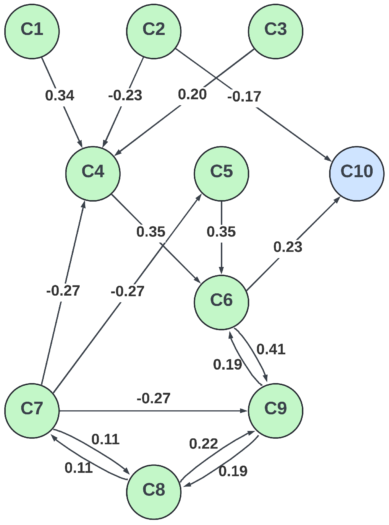
3.3. FCM Model Design

Regarding the construction of an FCM that describes the emotional cognition and behavioral logic of an individual in the face of a large-scale infectious disease, we needed to consider the nodes (concepts) and edges (weights) of the FCM separately. Mei et al., (2014) [24] trained an FCM model through Non-Linear Hebbian Learning (NHL) [34]. Using this model, a good performance was achieved in predicting the propagation characteristics of H1N1. We borrowed the concept setting from this model as well as the weights after training. For the concept setting, the concepts can be divided as:

• Inputs (e.g., cognition of the epidemiological situation).
• Internal status (e.g., emotions).
• Outputs, which need to be estimated for observation from outside.

These outputs are called Desired Output Concepts (DOCs), which are denoted by ${DOC}_i(i=1,\dots ,n_1,n_1<n)$. DOCs stand for the system factors and characteristics for which we want to estimate the values to describe the final state of the system. Suppose ${DOC}_i$ takes values in the range ${DOC}_i\in [{DOC}_i^{min},{DOC}_i^{max}]\subseteq [0,1]$ [24]. The specific concept settings, description, category, and initial value settings during simulation are shown in

Table 1. Individual Concepts Definition.

${\mathit{C}}_{\mathit{i}}$	Description	Category	Initial Value
$C_1$	Number of infected individuals	Input	0.0
$C_2$	Number of recovered individuals	Input	0.0
$C_3$	Health state of individual	Internal	0.0
$C_4$	Knowledge of local epidemic situation	Internal	0.0
$C_5$	Knowledge of global epidemic situation	Input	0.5
$C_6$	Epidemiological situation	Internal	0.0
$C_7$	Optimism level	Internal	0.0
$C_8$	Memory of situations	Internal	0.0
$C_9$	Instant reactions	Internal	0.0
$C_{10}\left(DOC\right)$ 1	Rate of getting influenced by the pandemic	Output	0.1

¹ $\beta$ in Equation (3).

.

The adjacent matrix or graph weight matrix setting of the FCM is subject to the one-way causality of a pair of concepts. Let us say that $C_1$ has a positive medium-strength causal effect on $C_4$, a process that can be represented as $w_{14}=0.34$. The specific weight matrix values are borrowed from Mei et al.’s [24] NHL training results in 2014, and the matrix representation is shown in Equation (4); the graph representation is shown in Figure 2.

$$W_{adj}=\left[\begin{array}{cccccccccc}0& 0& 0& 0.34& 0& 0& 0& 0& 0& 0\\ 0& 0& 0& -0.23& 0& 0& 0& 0& 0& -0.17\\ 0& 0& 0& 0.2& 0& 0& 0& 0& 0& 0\\ 0& 0& 0& 0& 0& 0.35& 0& 0& 0& 0\\ 0& 0& 0& 0& 0& 0.35& 0& 0& 0& 0\\ 0& 0& 0& 0& 0& 0& 0& 0& 0.41& 0.23\\ 0& 0& 0& -0.27& -0.27& 0& 0& 0.11& -0.27& 0\\ 0& 0& 0& 0& 0& 0& 0.11& 0& 0.22& 0\\ 0& 0& 0& 0& 0& 0.19& 0& 0.19& 0& 0\\ 0& 0& 0& 0& 0& 0& 0& 0& 0& 0\end{array}\right]$$

(4)

During the overall simulation process combined with the ABM, the Input concepts in the FCM representing each individual are first updated according to the changes in the external environment in the manner of Equation (5). Then, at the beginning of each simulation cycle, t, the updated $C_1$ and $C_2$ are used to calculate the remaining concepts (internal and output concepts) $C_j$ for the current cycle, in the manner of Equation (2).

$$\begin{array}{c}\hfill C_1^t=\frac{\# \mathrm{of} \mathrm{Confirmed} \mathrm{Cases} \mathrm{at} t}{\# \mathrm{of} \mathrm{all} \mathrm{agents}},\\ \hfill C_2^t=\frac{\# \mathrm{of} \mathrm{Recovered} \mathrm{Cases} \mathrm{at} t}{\# \mathrm{of} \mathrm{all} \mathrm{agents}}\end{array}$$

(5)

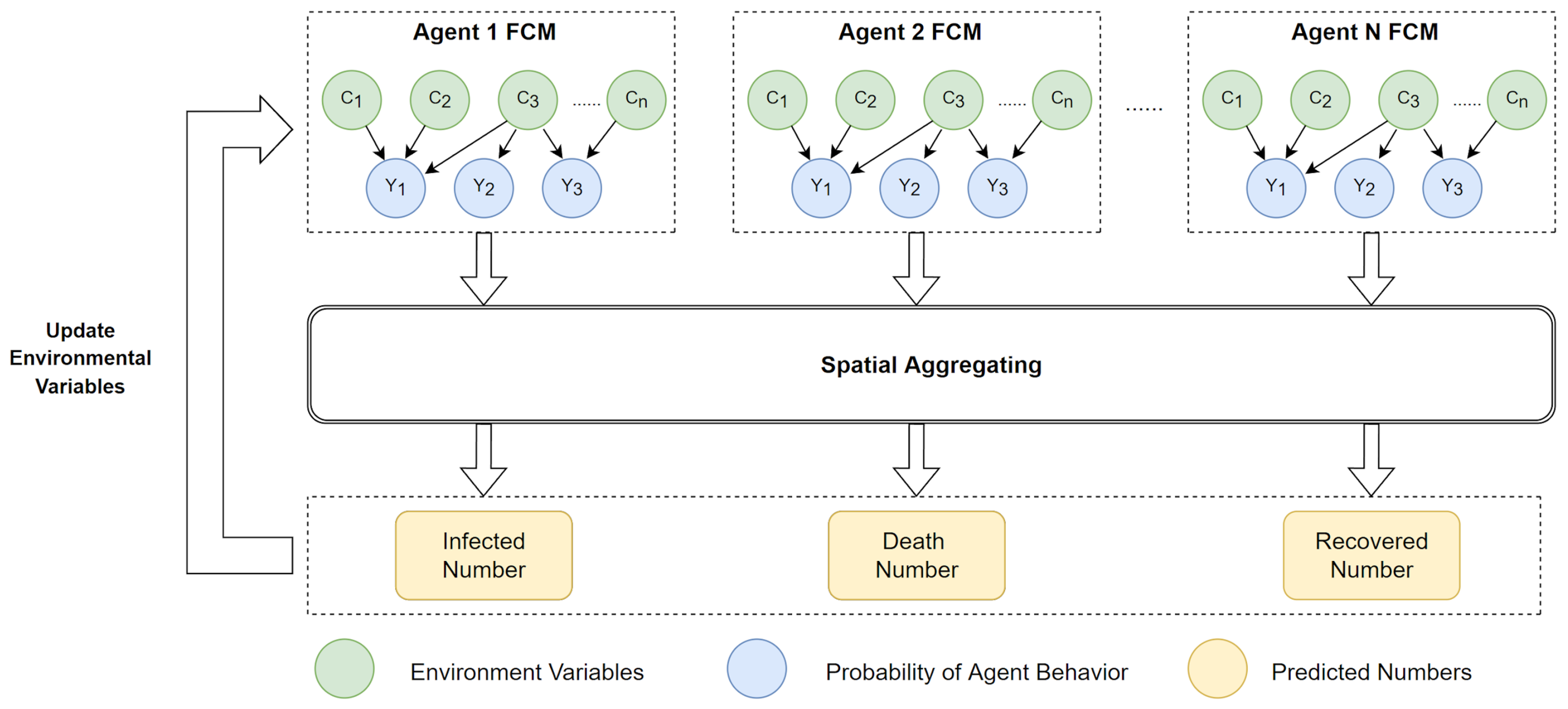
3.4. ABM and SEIR Model Design

Figure 3 illustrates the high-level design architecture of the FCM–ABM model simulating the SEIR process. We first initialize the hybrid FCM–ABM model by using the pre-trained FCM model mentioned above as a separate individual FCM for each agent. After that, the full simulated agents are distributed into each ward according to the population in the demographic dataset, and their neighbor relationship is established. The parameter settings are shown in

Table 2. ABM Simulation Parameters.

Category	Name	Description	Value
System Parameters	‘population’	Total population simulated	10,000
	‘days’	# of days in simulation	300
	‘iterations’	# of simulation iterations	20
Model Parameters	‘infect_rate’	Infectious Rate 1	0.2
	‘death_rate’	Disease Death Rate 2	0.0193
	‘recovery_days’	Average # of days to recover	7
	‘recovery_sd’	Standard deviation of ‘recovery_days’	3
	‘neighborhood_contact’	# of people met per person under local spread	40
	‘hotspot_contact’	# of people met per person under no intervention	120

¹ ${\alpha }_1$ in Equation (3). ² $\delta$ in Equation (3).

. Within each time node after the simulation is initiated, the algorithmic pseudo-code of the simulation process shown in Algorithm 1 is followed. It is important to note: the FCM of each agent is updated individually to determine the likelihood of each individual contracting the disease and recovering at each time point. Environmental factors at the current time point are updated by integrating all susceptible individuals in time and space. These updated factors will be used as FCM input concepts for each individual at subsequent time points. The key to closely aligning the ABM simulation process with the actual results is to ensure that the behavioral simulation of each agent accurately reflects the influence of the individual’s consciousness on his or her behavior. Individual FCM models are very effective in simulating this aspect. In each FCM loop, the notion of input of environmental variables reflects the influence of the environment on the individual. In turn, the significant impact that the individual has on the environment after integration is reflected in the individual’s output concepts, which allows the ABM simulation process to cycle successfully. The superiority of this design, in terms of its ability to integrate temporal and spatial properties, is demonstrated by the fact that each update of the FCM of the individual represented by the agent requires the combined influence of the local propagation properties of the ward in which it is located and the global propagation properties of the wards in its neighborhood. The approach used in this project comes closer to modeling the impact of individual consciousness on the broader epidemic transmission environment than the traditional ABM simulation SEIR model. As a result, it produces simulation predictions that are more realistic and reflective of the actual scenario.

Algorithm 1 FCM–ABM Simulating SEIR Pseudo-Code

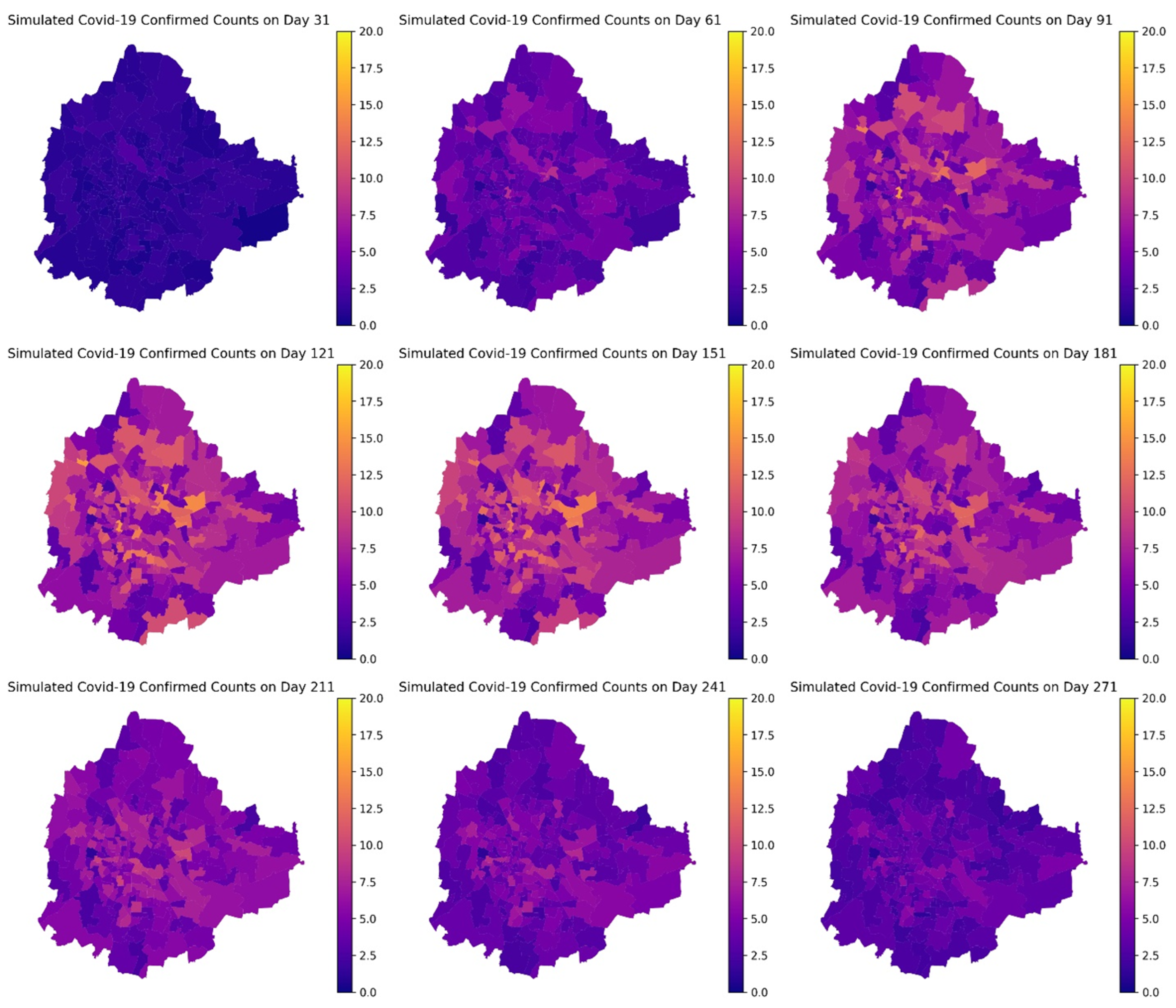
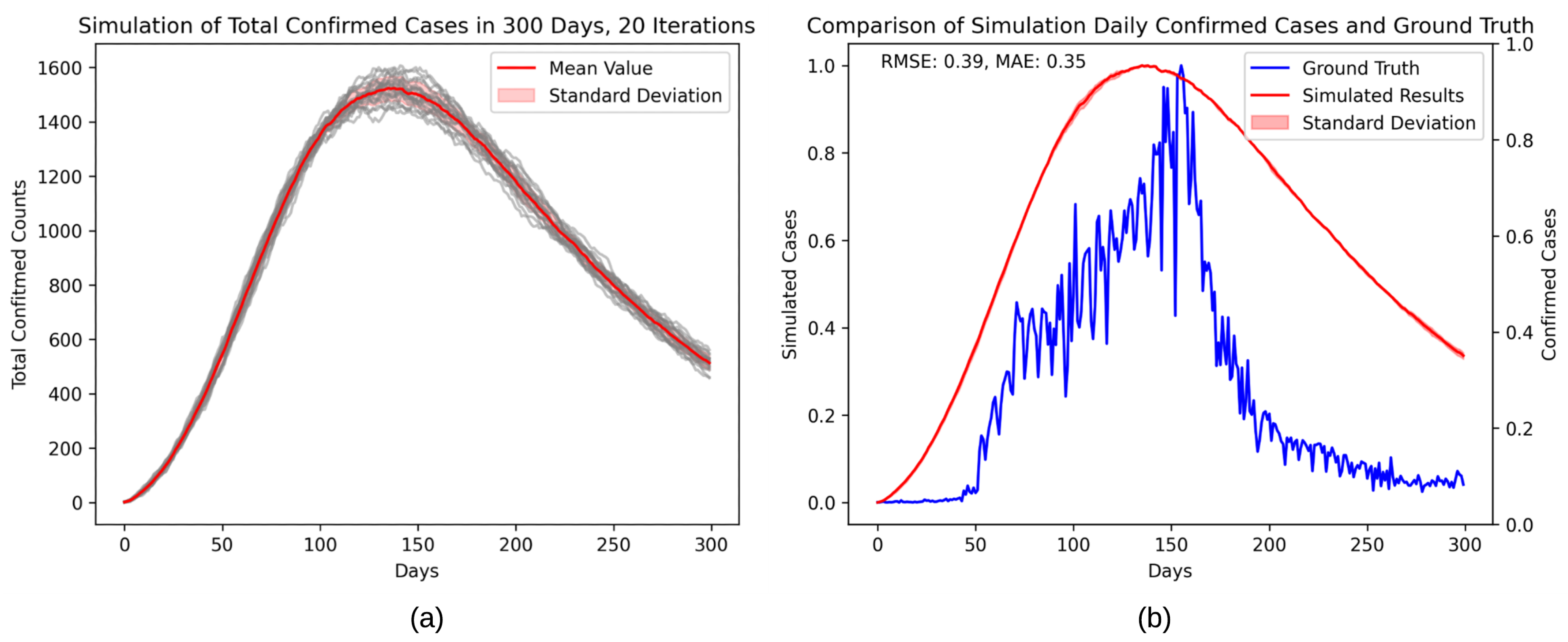
procedure input($FCM\left[\right],States\left[\right]$)     Initializing $FCM$ for all agents     Initializing $States\leftarrow$ ‘S’ for all agents     for $iter\in Iterations$ do         for $t\in Days$ do            for $i\in Population$ do                Update $FCM\left[i\right]$                $\beta \leftarrow FCM\left[10\right]$      ▹ Rate of getting influenced by the pandemic               if $States\left[i\right]==‘S’$ then                    if $random\left(\right)<\beta$ then                        $States\left[i\right]\leftarrow$ ‘E’                    end if                end if                if $States\left[i\right]==$ ‘E’ then                    if $hotspot$ then                   ▹ If current agent is in hotspot area                        while Iterate through $hotspot\_contacts$ do                           if $random\left(\right)<{\alpha }_1$ then                                ▹Infectious rate                               $States\left[i\right]\leftarrow$ ‘I’                           end if                        end while                    else                        while Iterate through $neighbor\_contacts$ do                           if $random\left(\right)<{\alpha }_1$ then                               $States\left[i\right]\leftarrow$ ‘I’                               $InfectDays\left[i\right]\leftarrow 0$                               $DaysNeedtoRecover\left[i\right]\leftarrow random\left(\right)$                           end if                        end while                    end if                end if                if $States\left[i\right]==‘I’$ then                    if $random\left(\right)<{\alpha }_2$ then                                             ▹Death Rate                        Delete $Agent\left[i\right]$                        Update $Stats\left[iter\right]\left[t\right]$                    else                        if $InfectDays\left[i\right]\ge DaysNeedtoRecover\left[i\right]$ then                           $States\left[i\right]\leftarrow$ ‘S’                        end if                    end if                end if                Update $Stats\left[iter\right]\left[t\right]$            end for         end for     end for     Return $Stats$ end procedure

4. Results

From 26 April 2020 (the first COVID-19 case recorded in the Bangalore urban area) to 19 February 2021, we modeled the COVID-19 transmission scenario in the Bangalore urban area for 300 days through 20 simulation iterations. Each iteration performed a separate dynamic FCM for the 10,000 simulated populations and ABM modeling for the whole. After obtaining the simulation results, we compared them with the factual statistics obtained in [29] to complete the evaluation of the simulation results.

The geodemographic graphs in Figure 4 provide a comprehensive visualization of the spatial-temporal progression of the pandemic, reflecting the diffusion and intensification of the virus within the district. From a temporal perspective, the initial 30 days of the simulation exhibit no discernible trend of an outbreak. However, from day 30 to day 180, there is a marked and rapid escalation in confirmed cases across all regions. Post day 180, a consistent decline in the number of confirmed cases is observed throughout the regions. The spatial distribution of cases evolves over time, with central areas consistently showing higher concentrations of confirmed cases. This could be indicative of higher population densities or varying degrees of adherence to public health guidelines. The patterns suggest that the central regions act as epicenters from which the virus propagates outward, affecting surrounding areas to varying degrees.

The simulation results of the model for the daily number of confirmed cases in the Bengaluru Urban District and its comparison with the ground truth are presented in Figure 5. It is clear that both the simulation results and the actual data, similar to the characteristics of most infectious diseases, show a typical ’S’-shaped curve for the number of confirmed cases on a single day of COVID-19: that is, there is an initial sub-exponential growth phase, a peak, and a subsequent decline phase. The peak in the mean trajectory shown in Figure 5a indicates that the number of cases peaks in the middle of the simulation period, after which the number of new cases begins to decline, suggesting that the outbreak may be under control or that it is failing. Some runs peak earlier, others later, and the height of the case count varies. The shaded area around the mean line represents the standard deviation at each time point, showing the variability or uncertainty in the simulation results. The blue line in Figure 5b shows considerable variability and several spikes, which may reflect actual reported anomalies or natural variations in disease spread. The red line follows the smooth bell curve typical of epidemiologic models, with a gradual decline after reaching a peak. The simulation results are very close to the actual data, in terms of trend changes in time and the points at which the peaks appear, suggesting that the simulation results reflect the general trend of the outbreak well. However, the gap between the simulation results and the actual data highlights the inherent complexity and unpredictability of real-world data.

5. Discussion

Spatiotemporal variables are modeled by introducing time series data and integrating socio-economic indicators, including population density, per capita income, availability of public health facilities, and population mobility. These factors are strongly correlated with a community’s resilience against large-scale pandemics [35], which enables us to capture the dynamic nature of epidemics. The spatiotemporal simulation results shown in Figure 4 exemplify that, by integrating these geospatial-temporal elements, our model can provide a detailed and accurate description of the spatial heterogeneity of a pandemic evolving in complex urban environments. The statistical analysis of the simulation results in Figure 5 captures the general trend of the outbreak well, with the peak of the simulated curve aligning closely with the highest concentration of actual cases. The simulation smooths out the finer details and fluctuations observed in the ground truth data, potentially due to the averaging effect of the model’s assumptions and parameters. The daily confirmed number of all wards reflects well the overall trend of the outbreak compared to the ground truth, including the time periods of the rising and descending phases and the temporal points when peaks occur.

However, there were some drawbacks in this work. First, in the overall statistical results, the decline phase of the number of COVID-19 cases, which is on the right-hand side of Figure 5, was faster in the ground truth than in the simulated results. This is due to the fact that the effects of sudden changes in virus mutations, vaccination or quarantine policies on individual immunity and infectious rates changes are not well captured [36,37]. Second, the input parameters of the FCM model used in this work were dynamically updated based on the run of the ABM model, but the weights of all FCMs were fixed by pre-training. This simplified modeling setup interpreted the differences in individual “cognitive-behavioral” logic because of the spatial heterogeneity in the socio-economic parameters of the community. In a real situation, more factors need to be taken into consideration, including age, occupation, cultural background, social support, etc. [38,39]. There is still room for improvement in the solution to the problem of modeling more realistically and effectively the heterogeneity of individual behavioral logic in epidemics. In addition, since the global outbreak in 2020, although several data platforms have been tracing and recording COVID-19 cases globally, developed by various agencies and research institutes (including the WHO [1], the New York Times [40], John Hopkins University [41], and the University of Illinois [42]), a common limitation shared by this work and similar projects in forecasting and analyzing epidemiological spatiotemporal patterns has been the need for high-quality and readily available daily updates [43]. Obtaining high-quality datasets at the sub-county level remains a challenge, making it difficult to evaluate spatiotemporal simulations quantitatively.

5.1. Future Work

Based on the limitations mentioned above, future optimization efforts should be focused on the following points. First, improving the model’s prediction accuracy in the time dimension and its robustness to sudden external changes. This includes not only incorporating more dynamic features, but also improving the model’s adaptation ability to rapidly changing environments. For instance, state-of-the-art time discretization techniques for time-fractional partial differential equations can provide more accurate predictions over extended periods, optimizing long-term accuracy in temporal dimensions [44]. Another aspect is to enhance the physical realism as well as the interpretability of the model in highly heterogeneous urban complex environments. This can be done by employing forward-retention and maximum-principle-retention numerical schemes [45,46] to maintain the physical consistency of the model. Finally, future research requires standardized, highly accurate epidemiological datasets with high spatial precision (sub-county level) as a publicly available standard for quantitatively evaluating spatiotemporal epidemiological prediction models. This could greatly facilitate the continued contribution of similar researchers on the same track.

5.2. Broader Impact

While many studies have focused on predicting COVID-19 cases and discovering spatiotemporal patterns [47,48,49], our work provides the field with new findings obtained from individuals’ behavior in an epidemic. These findings have important implications for public health strategies in urban areas. Quarantine policies and social distancing have proven effective in slowing the spread of COVID-19 [50,51]. Our model can inform interventions aimed at controlling the spread of infectious diseases in similar settings or other epidemiological contexts. By predicting disease spread under various scenarios, public health officials can better allocate medical resources, implement timely containment measures, and tailor public health policies to the specific dynamics of urban areas. Understanding how densely populated regions respond to different intervention strategies can lead to more effective and sustainable urban health management practices.

6. Conclusions

In this study, we applied FCM and ABM to explore the transmission dynamics of COVID-19. Our findings reveal complex transmission patterns consistent with real-world epidemiological data, but also highlight prediction biases, particularly for the Bengaluru Urban District. The use of FCMs allows for incorporating complex and uncertain factors (e.g., human behavior and policy changes) into the model consideration, which are often difficult to quantify. At the same time, ABM provides a fine-grained view of individual interactions and their potential role in disease spreading. The combination of FCM and ABM offers a new approach to understanding epidemic dynamics. Unlike traditional epidemiological modeling, this combined approach provides a more nuanced perspective that takes into account the uncertainty and variability inherent in human societies. This is particularly important for modeling diseases such as COVID-19, where community behavior and policy decisions can significantly impact epidemic trajectories. Taking population mobility in geographic space into account makes our model more robust to temporal heterogeneity in population distribution.

References

1. WHO COVID-19 Cases|WHO COVID-19 Dashboard. 2023. Available online: https://data.who.int/dashboards/covid19/cases (accessed on 12 March 2022).
2. Picoli, S.; Teixeira, J.; Ribeiro, H.; Malacarne, L.; Paupitz, R.; Mendes, R. Spreading patterns of the influenza A (H1N1) pandemic. PLoS ONE 2011, 6, e17823. [Google Scholar] [CrossRef] [PubMed]
3. Hunt, A. Exponential growth in Ebola outbreak since May 14, 2014. Complexity 2014, 20, 8–11. [Google Scholar] [CrossRef]
4. Maier, B.; Brockmann, D. Effective containment explains subexponential growth in recent confirmed COVID-19 cases in China. Science 2020, 368, 742–746. [Google Scholar] [CrossRef] [PubMed]
5. Kermack, W.; McKendrick, A. A contribution to the mathematical theory of epidemics. Proc. R. Soc. Lond. Ser. Contain. Pap. Math. Phys. Character 1927, 115, 700–721. [Google Scholar] [CrossRef]
6. Van Den Driessche, P.; Watmough, J. A simple SIS epidemic model with a backward bifurcation. J. Math. Biol. 2000, 40, 525–540. [Google Scholar] [CrossRef] [PubMed]
7. Liu, J.; Paré, P.; Du, E.; Sun, Z. A Networked SIS Disease Dynamics Model with a Waterborne Pathogen. In Proceedings of the 2019 American Control Conference (ACC), Philadelphia, PA, USA, 10–12 July 2019. [Google Scholar] [CrossRef]
8. Osman, M.; Adu, I.; Chen, Y. A simple SEIR mathematical model of malaria transmission. Asian Res. J. Math. 2017, 7, 1–22. [Google Scholar] [CrossRef]
9. Almeida, R. Analysis of a fractional SEIR model with treatment. Appl. Math. Lett. 2018, 84, 56–62. [Google Scholar] [CrossRef]
10. Bjørnstad, O.; Shea, K.; Krzywinski, M.; Altman, N. The SEIRS model for infectious disease dynamics. Nat. Methods 2020, 17, 557–558. [Google Scholar] [CrossRef]
11. de Lima, L.M.M.; de Sá, L.R.; dos Santos Macambira, A.F.U.; de Almeida Nogueir, J.; de Toledo Vianna, R.P.; de Moraes, R.M. A new combination rule for Spatial Decision Support Systems for epidemiology. Int. J. Health Geogr. 2019, 18, 24. [Google Scholar] [CrossRef]
12. Kosko, B. Fuzzy cognitive maps. Int. J. Man-Mach. Stud. 1986, 24, 65–75. [Google Scholar] [CrossRef]
13. Bonabeau, E. Agent-based modeling: Methods and techniques for simulating human systems. Proc. Natl. Acad. Sci. USA 2002, 99, 7280–7287. [Google Scholar] [CrossRef] [PubMed]
14. Kröger, M.; Schlickeiser, R. Analytical solution of the SIR-model for the temporal evolution of epidemics. Part A: Time-independent reproduction factor. J. Phys. Math. Theor. 2020, 53, 505601. [Google Scholar] [CrossRef]
15. Davis, C.; Giabbanelli, P.; Jetter, A. The Intersection of Agent Based Models and Fuzzy Cognitive Maps: A Review of an Emerging Hybrid Modeling Practice. In Proceedings of the 2019 Winter Simulation Conference (WSC), National Harbor, MD, USA, 8–11 December 2019. [Google Scholar] [CrossRef]
16. Chen, T.; Rui, J.; Wang, Q.; Zhao, Z.; Cui, J.; Yin, L. A mathematical model for simulating the phase-based transmissibility of a novel coronavirus. Infect. Dis. Poverty 2020, 9, 18–25. [Google Scholar] [CrossRef] [PubMed]
17. Li, Q.; Guan, X.; Wu, P.; Wang, X.; Zhou, L.; Tong, Y.; Ren, R.; Leung, K.; Lau, E.; Wong, J.; et al. Early transmission dynamics in Wuhan, China, of novel Coronavirus–Infected pneumonia. N. Engl. J. Med. 2020, 382, 1199–1207. [Google Scholar] [CrossRef] [PubMed]
18. Lyu, F.; Kang, J.; Wang, S.; Han, S.; Li, Z.; Wang, S. Multi-scale CyberGIS analytics for detecting spatiotemporal patterns of COVID-19. Hum. Dyn. Smart Cities 2021, 217–232. [Google Scholar] [CrossRef] [PubMed]
19. Perez, L.; Dragićević, S. An agent-based approach for modeling dynamics of contagious disease spread. Int. J. Health Geogr. 2009, 8, 50. [Google Scholar] [CrossRef] [PubMed]
20. Bian, L. A conceptual framework for an individual-based spatially explicit epidemiological model. Environ. Plan. Plan. Des. 2004, 31, 381–395. [Google Scholar] [CrossRef]
21. Giabbanelli, P.; Fattoruso, M.; Norman, M. CoFluences: Simulating the spread of social influences via a hybrid Agent-Based/Fuzzy cognitive maps architecture. In Proceedings of the 2019 ACM SIGSIM Conference on Principles of Advanced Discrete Simulation, Chicago, IL, USA, 3–5 June 2019. [Google Scholar] [CrossRef]
22. Dickerson, J.; Kosko, B. Virtual worlds as fuzzy cognitive maps. Presence Teleoperators Virtual Environ. 1994, 3, 173–189. [Google Scholar] [CrossRef]
23. Xirogiannis, G.; Stefanou, J.; Glykas, M. A fuzzy cognitive map approach to support urban design. Expert Syst. Appl. 2004, 26, 257–268. [Google Scholar] [CrossRef]
24. Mei, S.; Zhu, Y.; Qiu, X.; Zhou, X.; Zu, Z.; Boukhanovsky, A.; Sloot, P. Individual Decision Making Can Drive Epidemics: A Fuzzy Cognitive Map Study. IEEE Trans. Fuzzy Syst. 2014, 22, 264–273. [Google Scholar] [CrossRef]
25. Gilbert, G.; Troitzsch, K. Simulation for the Social Scientist. 1999. Available online: http://www.pensamientocomplejo.com.ar/docs/files/Gilbert%20and%20Troitzsch%20-%20Simulation%20for%20the%20social%20scientist.pdf (accessed on 10 May 2023).
26. Macal, C.; North, M. Tutorial on agent-based modelling and simulation. J. Simul. 2010, 4, 151–162. [Google Scholar] [CrossRef]
27. He, S.; Peng, Y.; Sun, K. SEIR modeling of the COVID-19 and its dynamics. Nonlinear Dyn. 2020, 101, 1667–1680. [Google Scholar] [CrossRef] [PubMed]
28. Weiss, H. The SIR model and the foundations of public health. Mater. Mat. 2013, 2013, 1–17. [Google Scholar]
29. Covid19india GitHub—Covid19india/Data. 2023. Available online: https://github.com/covid19india/data/ (accessed on 10 May 2023).
30. Tamrakar, V.; Srivastava, A.; Saikia, N.; Parmar, M.; Shukla, S.; Shabnam, S.; Boro, B.; Saha, A.; Debbarma, B. District level correlates of COVID-19 pandemic in India during March-October 2020. PLoS ONE 2021, 16, e0257533. [Google Scholar] [CrossRef] [PubMed]
31. Alam, S.; Schlecht, E.; Reichenbach, M. Impacts of COVID-19 on Small-Scale Dairy Enterprises in an Indian Megacity—Insights from Greater Bengaluru. Sustainability 2022, 14, 2057. [Google Scholar] [CrossRef]
32. Bauza, V.; Sclar, G.; Bisoyi, A.; Owens, A.; Ghugey, A.; Clasen, T. Experience of the COVID-19 pandemic in rural Odisha, India: Knowledge, preventative actions, and impacts on daily life. Int. J. Environ. Res. Public Health 2021, 18, 2863. [Google Scholar] [CrossRef] [PubMed]
33. OpenCity. BBMP Ward Information. OpenCity. 2020. Available online: https://data.opencity.in/dataset/bbmp-ward-information (accessed on 10 December 2023).
34. Papageorgiou, E.; Groumpos, P. A new hybrid method using evolutionary algorithms to train Fuzzy Cognitive Maps. Appl. Soft Comput. 2005, 5, 409–431. [Google Scholar] [CrossRef]
35. Nuzzo, J.; Meyer, D.; Snyder, M.; Ravi, S.; Lapascu, A.; Souleles, J.; Andrada, C.; Bishai, D. What makes health systems resilient against infectious disease outbreaks and natural hazards? Results from a scoping review. BMC Public Health 2019, 19, 1310. [Google Scholar] [CrossRef] [PubMed]
36. Zhou, Y.; Rahman, M.; Khanam, R. The impact of the government response on pandemic control in the long run—A dynamic empirical analysis based on COVID-19. PLoS ONE 2022, 17, e0267232. [Google Scholar] [CrossRef]
37. Khan, M.; Nazli, A.; Al-Furas, H.; Asad, M.; Ajmal, I.; Khan, D.; Shah, J.; Farooq, M.; Jiang, W. An overview of viral mutagenesis and the impact on pathogenesis of SARS-CoV-2 variants. Front. Immunol. 2022, 13, 1034444. [Google Scholar] [CrossRef]
38. Saeed, H.; Eslami, A.; Nassif, N.; Simpson, A.; Lal, S. Anxiety linked to COVID-19: A systematic review comparing anxiety rates in different populations. Int. J. Environ. Res. Public Health 2022, 19, 2189. [Google Scholar] [CrossRef] [PubMed]
39. Czepiel, D.; McCormack, C.; Da Silva, A.; Seblova, D.; Moro, M.; Restrepo-Henao, A.; Martínez, A.; Afolabi, O.; Alnasser, L.; Alvarado, R.; et al. Inequality on the frontline: A multi-country study on gender differences in mental health among healthcare workers during the COVID-19 pandemic. Glob. Ment. Health 2024, 11, e34. [Google Scholar] [CrossRef] [PubMed]
40. Times, N. Covid in the U.S.: Latest Maps, Case and Death Counts. 2023. Available online: https://www.nytimes.com/interactive/2021/us/covid-cases.html (accessed on 12 May 2024).
41. CSSEGISandData GitHub—CSSEGISandData/COVID-19: Novel Coronavirus (COVID-19) Cases, Provided by JHU CSSE. 2023. Available online: https://github.com/CSSEGISandData/COVID-19 (accessed on 12 May 2024).
42. University of Illinois at Urbana-Champaign WhereCOVID-19 by CyberGIS Center for Advanced Digital and Spatial Studies. 2020. Available online: https://wherecovid19.cigi.illinois.edu/ (accessed on 12 May 2024).
43. Abbasi, K. COVID-19: Fail to prepare, prepare to fail. J. R. Soc. Med. 2020, 113, 131. [Google Scholar] [CrossRef] [PubMed]
44. Yang, X.; Zhang, H. The uniform l1 long-time behavior of time discretization for time-fractional partial differential equations with nonsmooth data. Appl. Math. Lett. 2022, 124, 107644. [Google Scholar] [CrossRef]
45. Yang, X.; Zhang, H.; Zhang, Q.; Yuan, G.; Sheng, Z. The finite volume scheme preserving maximum principle for two-dimensional time-fractional Fokker–Planck equations on distorted meshes. Appl. Math. Lett. 2019, 97, 99–106. [Google Scholar] [CrossRef]
46. Yang, X.; Zhang, H.; Zhang, Q.; Yuan, G. Simple positivity-preserving nonlinear finite volume scheme for subdiffusion equations on general non-conforming distorted meshes. Nonlinear Dyn. 2022, 108, 3859–3886. [Google Scholar] [CrossRef]
47. Roosa, K.; Lee, Y.; Luo, R.; Kirpich, A.; Rothenberg, R.; Hyman, J.; Yan, P.; Chowell, G. Real-time forecasts of the COVID-19 epidemic in China from February 5th to February 24th, 2020. Infect. Dis. Model. 2020, 5, 256–263. [Google Scholar] [CrossRef] [PubMed]
48. Desjardins, M.R.; Hohl, A.; Delmelle, E.M. Rapid surveillance of COVID-19 in the United States using a prospective space-time scan statistic: Detecting and evaluating emerging clusters. Appl. Geogr. 2020, 118, 102202. [Google Scholar] [CrossRef] [PubMed]
49. Grasselli, G.; Pesenti, A.; Cecconi, M. Critical care utilization for the COVID-19 outbreak in Lombardy, Italy. JAMA 2020, 323, 1545. [Google Scholar] [CrossRef]
50. Anderson, R.; Heesterbeek, H.; Klinkenberg, D.; Hollingsworth, T. How will country-based mitigation measures influence the course of the COVID-19 epidemic? Lancet 2020, 395, 931–934. [Google Scholar] [CrossRef]
51. Wilder-Smith, A.; Freedman, D. Isolation, quarantine, social distancing and community containment: Pivotal role for old-style public health measures in the novel coronavirus (2019-nCoV) outbreak. J. Travel Med. 2020, 27, taaa020. [Google Scholar] [CrossRef] [PubMed]
Figure 1. Each concept denoted as C i , where C i possesses a state value labeled A i . This value A i may range within the interval [ 0 , 1 ] , signifying the level of activation of a concept or it can adopt a binary logic from the set 0 , 1 , indicating whether a concept is in an active (‘open’) or inactive (‘closed’) state. The weight ω i j of a directed link indicates the influence degree from the cause concept C i to the effect concept C j , which can be a fuzzy value with in [ 1 , 1 ] or a trivalent logic within −1, 0, 1 [24].
Sustainability 16 05036 g001
Figure 2. Individual FCM construction.
Sustainability 16 05036 g002
Figure 3. High-level design of SEIR model.
Sustainability 16 05036 g003
Figure 4. Geographic plots showing daily confirmed COVID-19 cases in ward level across the Bengaluru Urban District, in 300 days, at 30-day intervals. Colors range from purple (low) to orange (high), and the color bar quantifies case distribution, allowing easy comparison over time.
Sustainability 16 05036 g004
Figure 5. Comparative dynamics of simulated and actual daily COVID-19 case counts: (a) Mean and standard deviation of the simulation results for the number of new diagnoses per day over 20 periods, after smoothing with a sliding window of length 8. The red line represents the average trajectory of disease transmission over 20 iterations. The grey lines represent individual iterations, showing the variation in each simulation run. Wider shaded areas indicate greater variability between individual iterations. (b) Comparative analysis of COVID-19’s simulated daily confirmed cases versus actual reported data (i.e., “ground truth”) over 300 days. The blue line indicates the daily fluctuations in recorded confirmed cases. The red line indicates the simulation results. The pink shaded area represents the standard deviation of the simulated results, indicating the variability of the simulated data.
Sustainability 16 05036 g005