Analysis of Land Use Change and Its Economic and Ecological Value under the Optimal Scenario and Green Development Advancement Policy: A Case Study of Hechi, China

Abstract

Studying future land use change for sustainable regional development remains a challenging task. Although many previous studies have conducted multi-scenario simulations, research on optimal scenarios that consider the impact of regional policies is relatively limited. In this paper, based on exploring the drivers of land use change, a land value assessment framework that considers the impacts of future land use change is developed by combining multi-objective programming and patch-generating land use simulation models. The framework is useful for predicting land use changes and assessing the ecological and economic values of land in different development strategy contexts (natural development scenario, economic development scenario, ecological protection scenario and green economy scenario). The results show that during the period 1990–2020, the forest area fluctuated greatly. The area of forest initially increased from 249.21 × 10⁴ hm² to 249.33 × 10⁴ hm², but then decreased to 248.53 × 10⁴ hm². Moreover, the model results show that altitude is the main driving force of land use change. By 2035, the economic value under the green economy scenario will be CNY 924.08 × 10⁸, slightly lower than the CNY 938.01 × 10⁸ under the economic development scenario. However, the ecological value under the economic development scenario will drop from CNY 675.43 × 10⁸ CNY in 2020 to CNY 633.56 × 10⁸ in 2025. Therefore, the green economy scenario will be more in line with the development needs of local policies, and the future land use distribution of this scenario can provide reference for regional land planning.

1. Introduction

Rationalized land use allocation is expected to result in more balanced economic and ecological values. The cumulative effects of localized changes in land use have far-reaching ramifications for the life-support functions of the planet and human livelihoods [1]. Given its importance, land use change has become a focus of attention for many international organizations and countries [2,3]. For example, the International Geosphere-Biosphere Program (IGBP) and the International Human Dimensions Program on Global Environmental Change (IHDP) established a land use and land cover change (LUCC) research program in the 1990s to mitigate a range of issues arising from climate change and ecological evolution. The land conservation targets are also encompassed by the Sustainable Development Goals (SDGs) adopted in 2015 as part of the United Nations’ 2030 Agenda for Sustainable Development [4]. In China, measures such as converting farmland into forests, land management laws, green agriculture, and ecological civilization construction aim to, among other things, alleviate the adverse impacts caused by irrational land use changes [5,6]. In particular, the Green Development Advancement Policy (GDAP), a local policy that rationally develops and utilizes locally advantageous resources to promote economic development, has the main goal of promoting local economic development while maximizing the restoration and protection of the environment through activities related to six aspects: industry, infrastructure, consumption, the attainment of carbon peaking and carbon neutrality, finance, and ecological civilization construction [7]. It is possible to provide valuable insights for regional planning by predicting future land use changes. To date, numerous scholars have undertaken a series of studies to predict land use changes [8,9,10]. For instance, Hu et al. [11] estimated land use changes and ecosystem service values (ESVs) in Anhui Province spanning the 1995–2030 period. Meanwhile, Peng et al. [12] forecasted the future pattern of changes in natural wetlands under the optimal scenario. Zhu et al. [13] combined resource environmental carrying capacity (RECC) with land use change (LUC) to study and optimize the spatial pattern of land use in Zhengzhou from 2000 to 2030. However, many prior studies have failed to comprehensively explore optimal future scenarios and have been somewhat deficient in identifying the potential drivers of land use change [14]. In order to fill this gap, we define the optimal scenario as a development model that promotes local economic development while maximizing the recovery and protection of the environment, and measure the best scenario by using ecological value and economic value. The land use forecasting simulation model comprises two components: scenario design, which addresses regional requirements, and a spatial distribution model that facilitates the prediction of distribution [10]. The scenario design is devoted to forecasting the demand for different types of land use, with a detailed analysis of the potential developmental trajectories within the study area. While approaches such as Markov chains [15] and the gray model (GM(1,1)) [11] necessitate only historical land use changes to project future land demand, their applicability is confined to straightforward scenarios [16]. In contrast, the system dynamics (SD) model comprehensively incorporates objective factors, including social and climatic considerations [10]. Nevertheless, the widespread adoption of the SD model is constrained by its inherent complexity [12,17]. With this limitation in mind, the multi-objective planning (MOP) approach has emerged as a scenario design methodology that optimizes an objective function to generate a land use structure that best meets decision-makers’ requirements [18]. This approach has the advantage of incorporating objective factors while remaining relatively simple and easy to implement [9,19].

Among spatial allocation models, scholars mostly apply the FLUS model [20], the CLUE-S model [21], the CA-Markov model [22] and the PLUS model [23]. In terms of simulation and prediction, these models have their own advantages and disadvantages. For example, the CLUE-S model is well integrated, but the influence of natural and policy factors is not fully considered. The CA-Markov model can predict the total amount of transfers and the transfer probability matrices of different land use types. Nevertheless, the relationship between the spatial location of land use and its driving factors is complicated and nonlinear. Thus, it is difficult for the CA-Markov model to determine the transition rules of land use change [24,25]. Compared with the cellular automata (CA), FLUS models, and CLUE-S, patch-generating land use simulation (PLUS) models can effectively address the nonlinear relationships between drivers and land use types [23], mine the transformation rules and simulate dynamic changes in patches [26]. Therefore, combining the MOP and PLUS models to simulate and predict land use change can efficiently identify the main drivers of land use change. In addition, the spatial pattern can be reconstructed according to the simulation results to ensure that the simulated land use is close to the expectation.

Many prior studies have failed to comprehensively explore optimal future scenarios and have been somewhat deficient in identifying the potential drivers of land use change. To address this gap, this paper aims to thoroughly explore land use changes and their drivers under the optimal scenario, and to conduct further research on the values derived from land change. Specifically, this study can accurately predict the detailed situation of land use quantity and distribution in the optimal scenario by establishing a research framework that effectively integrates MOP and PLUS models. This innovative approach enhances the ability to support sustainable regional development and provides valuable insights for regional land management.

2. Research Methodology

This study presents a detailed workflow (see Figure 1). It predicts future land use changes from 2020 to 2035 and evaluates the economic and ecological values under corresponding scenarios. Firstly, the data were processed. Secondly, under the policy background of GDAP, the specific planning documents relating to GDAP were quantified into multi-objective planning and combined with the Markov chain method, four scenarios were proposed, and the future land use pattern was predicted. In the end, the value of the land was evaluated.

2.1. PLUS Model

2.1.1. Land Expansion Analysis

The PLUS model is an evolutionary version based on the FLUS model, which considers the policy-driven bootstrapping role and focuses on patch-level fine-grained land use prediction [27]. First, by overlaying the land use data of two periods and extracting the state change cells from the later data, these cells represent the areas of change in various land use types. Then, suitability maps for various land use categories were generated through application of the random forest classification algorithm. The algorithm takes 16 driving factors as independent variables and land use as dependent variables. When the training samples were created, the sample size was set to 1% of the total land use pixels. The number of randomly selected features (mTry) and the decision tree (n Tree) were also specified as key parameters [28]. The mTry was set to four, as it is often a third or square root of the total number of features [29]. The efficiency and accuracy of calculations are affected by the nTree value. A higher nTree value results in higher precision but lower speed. We set this value to 40 [11].

2.1.2. Land Use Prediction Module

The PLUS model’s land use prediction module incorporates “bottom-up” (i.e., local land-use competition) and “top-down” (i.e., land-use demand) effects [30]. When the simulation is carried out, the number of the simulated land reaches the expected value by constantly changing the regional land-use competition mechanism [31]. Before running the PLUS model, various parameters need to be adjusted, which mainly include the following:

(1) Neighborhood weight: the value 0 to 1 is used to express the potential for expansion of various land uses. Land use types with a higher value have a greater expansion capacity. In order to obtain the neighborhood weight, we first calculated the proportion of the expansion area of six land use types in relation to the total expansion area for 1990 to 2020 [8,24]. Then, we adjusted the neighborhood weight for the different scenarios by combining personal experience, referring to other studies [24,32] and exploiting expert knowledge. Through several simulations, we selected the parameters that had the highest accuracy and were most similar to the future number of land requirements, as shown in

Table 1. Neighborhood weights set for each scenario.

	Cropland	Forest	Grass	Water Area	Built-Up Land	Bare Land
Natural development scenario (NDS)	0.6	0.74	0.47	0.9	0.8	0.1
Economic development scenario (EDS)	0.5	1	0.5	0.9	0.5	0.1
Ecological protection scenario (EPS)	0.7	0.4	0.1	0.5	1	0.1
Green economy scenario (GES)	0.5	0.9	0.5	0.8	0.7	0.1

.

(2) Conversion matrix: the conversion matrix is a square matrix with n rows and n columns; the value in the corresponding matrix is 1 if a land use type can be transformed to another, otherwise, it is 0 [33]. In the natural development scenario, there is no restriction on the conversion matrix. The economic development scenario restricts the conversion of cropland and construction land, considering that these two types of land are the main origin of economic value. Grassland, forest and water areas are not converted in the ecological protection scenario. In the green economy scenario, the other three scenarios are comprehensively considered. We convert the conversion matrix into a conversion diagram for viewing (Figure 2).

(3) Spatial constraints: spatial constraints refer to specific areas where land use cannot be altered, such as national parks and nature reserves [34]. In this study, we constructed spatial constraints by creating a 60 m buffer zone around the watershed and combining it with the World Database on Protected Areas. The setting of the 60 m buffer zone conforms to both the literature experience and local regulations. Notably, spatial constraints were set for only the ecological-protection and green-economy scenarios of the PLUS model.

(4) Demand area: the required area is a crucial parameter for determining whether PLUS will halt iteration. It refers the to the land use area of the target year [35]. In this paper, it is calculated by MOP; see Section 2.3 for details.

Then, the detailed patterns of land use types are repeatedly simulated by using the PLUS model. The model will stop iterating when the simulated area is roughly the same as the required area, within the appropriate range.

2.2. Accuracy Verification

Land use data were used for validation of the PLUS model to make sure it was accurate. Specifically, we used 1990–2005 land use data to predict 2020 land use and contrasted it with the actual 2020 land use map. Overall accuracy and the Kappa coefficient were used to measure model accuracy. Overall accuracy is the proportion of correctly classified pixels to all pixels [36,37]. Its calculation formula is

$$P_{OA}=\frac{{{\displaystyle \sum }}_{i=1}^k{P}_{ii}}{N}\times 100\%$$

(1)

where P_ii is the number of pixels correctly classified in the specified land use (i) and N denotes the total number of pixels.

The kappa coefficient reflects the degree of agreement between the simulated image and the real image, and it is an objective evaluation standard for testing the consistency of the two images. The formula is

$$K=\frac{N{{\displaystyle \sum }}_{i=1}^m{P}_{ii}-{{\displaystyle \sum }}_{i=1}^m\left(P_{pi}\times P_{qi}\right)}{N^2-{{\displaystyle \sum }}_{i=1}^m(P_{pi}\times P_{qi})}$$

(2)

where P_pi is the total number of pixels of class i in the real image and P_qi is the total number of pixels of class i in the simulated image.

In this study, the map’s overall accuracy in 2020 was found to be 0.97, with a kappa coefficient of 0.92, indicating that the simulation results are more accurate.

2.3. Use of MOP to Generate Land Use Scenarios

2.3.1. Scenario Design

Multi-objective programming (MOP) is an open and flexible approach that can be applied to a wide range of environmental and macroeconomic policies [38]. By appropriately defining objective optimization functions and constraints, we can consider expectations and variables relevant to planners, such as future economic conditions and food demand. This study refers to the objective optimization functions of other scholars [9,39]. The purpose is to quantify the clear requirements for future development in GDAP and related policies within the following scenario design. The MOP method was used to develop three scenarios for the target year 2035, namely, the economic development scenario (EDS), the ecological protection scenario (EPS), and the green economy scenario (GES), taking into account local policies. Additionally, the Markov chain method was used to construct a natural development scenario (NDS) for comparison with the other three scenarios. These scenarios were selected for analysis because they provide a comprehensive understanding of the trade-offs and synergies between ecological and economic values in land use change. Among the various scenarios, there is an “optimal scenario” in the future which is expected to present high economic and ecological benefits and a positive growth trend.

The NDS is a baseline scenario that does not take into account unforeseen policies or natural disasters, also known as the unconstrained development scenario. Land use continues to develop according to historical trends under this scenario. We used land use maps from 2005 and 2020 and applied the Markov chain method to calculate future land requirements.

EDS takes economic value as the primary consideration and emphasizes economic growth; future land use changes are based on social and economic development. In order to quantify the scenario, the following objective function is established:

$$f_1\left(x\right)=max{{\displaystyle \sum }}_{i=1}^6{a}_i\times x_i=\max \left(a_1{x}_1+a_2{x}_2+a_3{x}_3+a_4{x}_4+a_5{x}_5+a_6{x}_6\right)$$

(3)

where x_i is the land use area and a_i is the economic coefficient, which is calculated by dividing the industrial value by the area of land use. The economic coefficient is calculated as follows: $a_1$ represents the economic coefficient of cropland, which is obtained by dividing the value of agricultural production by the area of cropland, which is equal to 4.03. $a_2$ represents the economic coefficient of forest, which is equal to 0.14, which is obtained by dividing the value of forestry production by the area of forest. Due to the low level of local livestock production, we set the value of grassland at 10% the value of livestock production, and, finally, we obtained $a_3$ as 0.28. The value of the water area is calculated according to the fishery production, and after calculation we obtain $a_4$ as equal to 2.61. The ratio of the sum of the output values of the primary and secondary industries to the construction land area is $a_5$, which is calculated to be 247.52. The economic value of bare land is set to 0, and $a_6$ is equal to 0. EPS prioritizes the protection of the environment over economic development. In case of conflict between the two, priority must be given to the ecosystem. Future land use changes should be based on environmental protection. The objective function is defined as follows:

$$f_2\left(x\right)=max{{\displaystyle \sum }}_{i=1}^6{b}_i\times x_i=max\left(b_1{x}_1+b_2{x}_2+b_3{x}_3+b_4{x}_4+b_5{x}_5+b_6{x}_6\right)$$

(4)

where b_i is the ecological coefficient, obtained by calculating the ecosystem service value of land use. We referred to the research of Xie et al. [40] to calculate this parameter. Importantly, in calculating the ecological coefficient of land use, we exclude the value of services that have both economic and ecological attributes, such as food production. This ensures that only ecological service values are considered. Finally, $b_1$ equals 0.39, $b_2$ equals 2.63, $b_3$ equals 2.06, $b_4$ equals 6.65, $b_5$ equals 0 and $b_6$ equals 0.15.

The GES aims to maximize ecological benefits while considering economic development. Its objective is to achieve an optimal balance between economic and ecological values. The objective function is expressed as follows:

$$f_3\left(x\right)=max\left\{\alpha \times f_1\left(x\right)+\left(1-\alpha \right)\times f_2\left(x\right)\right\}$$

(5)

where α represents the weighting coefficient, which we adjust in increments of 0.01 to calculate the land use area under different weights. We observed that when α is 0.31 or 0.34, the $x$ values (10⁴/hm²) are 35.75, 249.8, 42.04, 4.25, 2.92 and 0.0026, while the x values obtained by other weights are unchanged; they are 30.91, 249.8, 46.88, 4.25, 2.92 and 0.0026, respectively. As when α is 0.31 or 0.34 the obtained $x$ is more in line with the historical trend, we consider choosing the weight α as 0.31 or 0.34. We completed the calculation of this part by using lingo11 software. Considering the concept of ‘ecological priority’ emphasized in many planning documents of Hechi City, we chose α = 0.31.

2.3.2. Constraint Conditions

Cropland constraints: over time, the grain provided by cropland should exceed consumption. According to the “Master Plan of Hechi City (2016–2035)”, by 2035, the population will reach 5.3 million, the per capita grain consumption will reach 144.95 kg/person, the cultivated land output will reach 3915 kg/hm², and the planting rate will reach 63.49%. Therefore, we set the lower limit of cultivated land to 30.91 × 10⁴ hm². From 1990 to 2020, the total cultivated land area decreased, and the “14th Five-Year Plan for the Agricultural and Rural Modernization Development of Hechi City” proposed implementing a new round of returning farmland to forests and grasslands; thus, the upper limit of cultivated land was set as the predicted value of the Markov chain.

$$30.91\times {10}^4\le x_1\le 38.98\times {10}^4$$

(6)

Forest constraints: the “14th Five-Year Plan for the Ecological and Environmental Protection of Hechi City” aims to achieve a forest cover of at least 71.52% by 2025. Based on the 1.02% increase in coverage from 2015 to 2020, we predicted that the forest coverage in 2035 will be no less than 72.57%, resulting in a forest area of at least 242.94 × 10⁴ hm². The upper limit of forest growth is set at a historical high of 249.80 × 10⁴ hm².

$$30.91\times {10}^4\le x_1\le 38.98\times {10}^4$$

(7)

Grassland constraints: the “Guiding Opinions of the General Office of the People’s Government of the Guangxi Zhuang Autonomous Region on Supporting the Construction of Hechi City into a Pilot Green Development Area” advocates ecological priority and green development. On this basis, it is predicted that the grassland area will stabilize or increase in the future; thus, the upper limit of grassland is set at 47.32 × 10⁴ hm² (1995 data), and the lower limit is set at 42.04 × 10⁴ hm² (the grass area in 2035 predicted by the Markov chain).

$$42.04\times {10}^4\le x_3\le 47.32\times {10}^4$$

(8)

Water area constraints: since 1990, the watershed area has shown an increasing trend. Therefore, we set the lower water area constraint for 2035 to 30.76 × 10⁴ hm² (which was the water area in 2020) and the upper constraint to 42.51 × 10⁴ hm² (which is 120% of the Markov chain-projected water area in 2035).

$$30.76\times {10}^4\le x_4\le 42.51\times {10}^4$$

(9)

Built-up land constraints: The area of built-up land was projected to be between 1.95 × 10⁴ hm² (80% of the Markov chain projection for built-up land in 2035) and 2.92 × 10⁴ hm² (120% of the Markov chain projection for built-up land in 2035).

$$1.95\times {10}^4\le x_5\le 2.92\times {10}^4$$

(10)

Bare land constraints: Considering that urban development often takes up bare land, we set its upper limit at the bare land area in 2020 and the lower limit at 50% of the same area.

$$0.0023\times {10}^4\le x_6\le 0.0047\times {10}^4$$

(11)

Total area constraint: The total land use area in 2035 should be equal to the area in 2020.

$$x_1+x_2+x_3+x_4+x_5+x_6=334.76\times {10}^4$$

(12)

2.4. Land Value Assessment

The evaluation of the economic and ecological value of land use change can comprehensively evaluate the trade-offs between different development scenarios. This method also embodies the core concept of GDAP, that is, “green development”, using ecological value to consider “green” and economic value to analyze “development”. The calculation of the economic and ecological value of land use is based on the procedure in Section 2.3.1, and the formula for the economic and ecological value is as follows:

$$f_1\left(x\right)={{\displaystyle \sum }}_{i=1}^6{a}_i\times x_i=\left(4.03x_1+0.14x_2+0.28x_3+2.61x_4+247.52x_5+0x_6\right)$$

(13)

$$f_2\left(x\right)={{\displaystyle \sum }}_{i=1}^6{b}_i\times x_i=\left(0.39x_1+2.63x_2+2.06x_3+6.65x_4+0x_5+0.15x_6\right)$$

(14)

where $f_1\left(x\right)$ is the economic value, $a_i$ is the economic coefficient, $f_2\left(x\right)$ is the ecological value, and $b_i$ is the ecological coefficient. The variable $x_i$ is the land category.

3. Materials and Methods

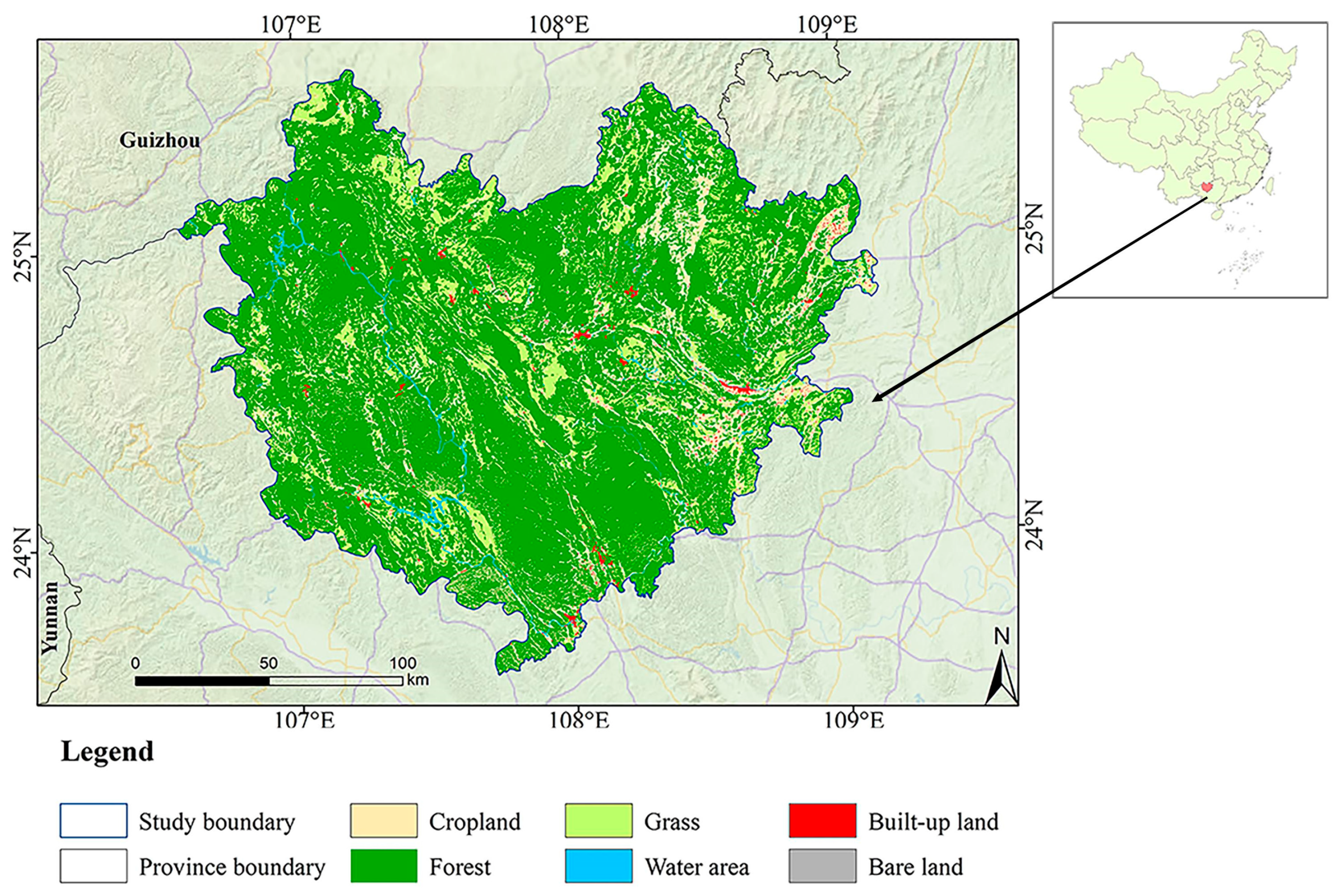
3.1. Study Area

Hechi is in the northwestern region of Guangxi, situated at the southern edge of the Yunnan–Guizhou Plateau. As such, it represents a crucial passageway between the southwest and the coastal regions. The geographic coordinates are between 106°34′ E and 109°09′ E and 23°41′ N and 25°37′ N, with an east–west length of 228 km, a north–south width of 260 km, and a total area of 33,500 square kilometers (Figure 3). The area lies in the low-latitude zone and is subject to the subtropical monsoon climate. Average annual temperatures range from 16.9 to 21.5 °C. The average annual rainfall is usually 1200–1600 mm, the summers are long and hot, the winters are short and warm, and there is sufficient light and a long frost-free period, which is favorable for the growth of crops. With many high mountains, little arable land and an extensive karst distribution, Hechi is a major karst landscape distribution area, with a karst landscape area of 21,800 square kilometers, accounting for 65.74% of the city’s land area [41]. As an important ecological barrier in the northwest, Hechi bears a major responsibility for maintaining ecological security; however, it is also an underdeveloped and resource-oriented region. Therefore, accelerating economic transformation and consolidating and expanding the results of poverty alleviation are arduous tasks. The findings of this study can serve as a reference for land planning in underdeveloped regions, and can also provide a reference for other areas that implement similar GDAP policies [42].

3.2. Data Sources and Processing

The 1990, 2005 and 2020 land use data used in the paper came from the Resource Environment and Science Data Center of the Chinese Academy of Sciences. These data have a spatial resolution of 30 m. We reclassified the land use into six first-level classifications and combined these with field surveys to modify obviously erroneous pixels; the precision of the comprehensive evaluation of the final first-level types reached more than 93%.

Sixteen driving factors were also collected from socio-economic, climatic and environmental factors. They were collected in such a way that the time period of each driver was as close as possible to that of the land use data [43]. The socioeconomic factors included population, GDP, the distance from the county government and various roads (including the distance from national roads, provincial roads, highways, railroads, secondary roads, and tertiary roads). Climatic and environmental factors included the average annual temperature, annual precipitation, the soil type, soil-erosion intensity level, the digital elevation model (DEM), slope, and the distance from water. Various distances to roads and waters were calculated by the Euclidean distance method. Furthermore, we gathered statistical indicators including population, GDP and national average prices, as well as the acreage devoted to cultivating rice, soybeans, and other crops from the Guangxi Provincial Statistical Yearbook and the Compendium of Agricultural Costs and Benefits in China. We generated a 60 m buffer zone around the water system and referred to the World Database on Protected Areas [44] to establish spatial constraints for the PLUS model.

Table 2. Data used in this study and their detailed information.

Category	Index	Original Resolution	Period	Data Resources
Land use/cover	Land use/cover	30 m	1990–2020	https://www.resdc.cn/ (accessed on 13 August 2023)
Socioeconomic drivers	Population	1 km	2019	https://www.resdc.cn/ (accessed on 13 August 2023)
	GDP	1 km	2019	https://www.resdc.cn/ (accessed on 13 August 2023)
	Proximity to governments	\	2020	https://lbs.amap.com/tools/picker (accessed on 20 August 2023)
	Proximity to national highways	\	2020	https://www.webmap.cn/ (accessed on 5 September 2023)
	Proximity to provincial highways	\	2020	https://www.webmap.cn/ (accessed on 5 September 2023)
	Proximity to highways	\	2020	https://www.webmap.cn/ (accessed on 5 September 2023)
	Proximity to railways	\	2020	https://www.webmap.cn/ (accessed on 5 September 2023)
	Proximity to secondary roads	\	2020	https://www.webmap.cn/ (accessed on 5 September 2023)
	Proximity to tertiary roads	\	2020	https://www.webmap.cn/ (accessed on 5 September 2023)
Climatic and environmental drivers	Annual mean temperature	1 km	2020	https://www.resdc.cn/ (accessed on 13 August 2023)
	Annual precipitation	1 km	2020	https://www.resdc.cn/ (accessed on 13 August 2023)
	Soil type	1 km	1995	https://www.resdc.cn/ (accessed on 13 August 2023)
	Soil-erosion intensity level	1 km	1995	https://www.resdc.cn/ (accessed on 13 August 2023)
	Elevation	30 m	\	http://www.gscloud.cn (accessed on 6 September 2023)
	Slope	30 m	\	http://www.gscloud.cn (accessed on 6 September 2023)
	Proximity to open water	\	2020	https://www.webmap.cn/ (accessed on 5 September 2023)

shows the details of the data used in the study.

4. Results

4.1. Land Use Change, 1990–2020

Figure 4 provides detailed information on land use changes. The area of cropland decreased from 39.80 × 10⁴ hm² to 39.25 × 10⁴ hm² because of the implementation of returning farmland to forests and lakes. In contrast, the area of forest initially increased from 2,492,061.66 hm² to 249.33 × 10⁴ hm² but then decreased to 248.53 × 10⁴ hm². The conversion of forestland into cropland was most significant between 1990 and 2005. The terrain of Hechi is undulating, and high-quality cropland is scarce. Part of the increase in cropland is due to terraces formed by forest clearing. Additionally, factors such as increased demand for timber due to accelerated urbanization and wetland restoration contributed to the decline in the area of forested land. The grassland area experienced a decrease followed by a rebound, resulting in no significant overall change. In contrast, the water area grew from 2.16 × 10⁴ hm² in 1990 to 3.08 × 10⁴ hm² in 2020, representing a growth rate of 42.17%. This faster growth rate can be attributed to Hechi’s commitment to ecological priority and green development, as well as its active implementation of wetland protection and restoration policies. In 1990, the area of built-up land was 1.13 × 10⁴ hm². By 2005, it had increased by 1340.01 hm², and by 2020, it had rapidly increased to 1.87 × 10⁴ hm². The area of bare land exhibited a downward trajectory.

4.2. Potential Drivers of LUCC

The analysis of the drivers of land use change using the PLUS model is more rigorous and explicit than that used in previous studies. The PLUS model combines all shifts “from” one land use type “to” another land use type. As a result, there is a clearer measure of variable importance, which can be understood as the contribution of multiple driving factors to the process of transformation of other land use types to a specific target land-use type.

Figure 5 and Figure 6, respectively, show the expansion of four land use types and the contribution of various variables to land growth from 1990 to 2020. Specifically, elevation is the main driver of cropland expansion, with a contribution value of 0.087. Cropland expansion mainly occurs in areas at lower elevations and, considering the prevalence of karst landscapes in the Hechi region, most semi-mountainous areas are unsuitable for the development of terraces; thus, new cropland is distributed in areas with gentler terrain. This factor is followed by GDP, whose contribution value is 0.082, indicating that most cropland expansion occurs in places where human activities are intensive. The distance to the county government has the largest effect on forestland change, with a contribution value of 0.089. For forests, by overlaying forestland growth with proximity to the administrative center, we find that new forestland is mainly distributed in areas farther from the government. In addition, forest growth was strongly correlated with the distance to secondary roads, suggesting that forest growth may be influenced by anthropogenic management. Temperature is also an important factor influencing forest growth, with a contribution value of 0.088. Because Hechi is located in the southern region and has a high degree of relief and because the main forest types in the region are fir and pine, which prefer milder environments, forest growth occurs mainly on semi-mountainous slopes, where temperatures are more favorable. The main driver of grassland expansion is elevation, which has a contribution value of 0.152, and the expansion areas are mainly located on semi-mountainous slopes and hills. In addition, our findings indicate that built-up land growth is most affected by the distance from the county government, followed by that from secondary roads, with respective contribution values of 0.182 and 0.125. The distribution of built-up land growth has a high overlap with the location of the county government, as most emerging cities expand outward from the city center, and construction sites spreading out from the periphery are usually built with accessibility in mind. Overall, in the ranking of the values of the contributions to different land use changes, elevation is in the forefront, indicating that elevation is an important driving factor of land use change in this area.

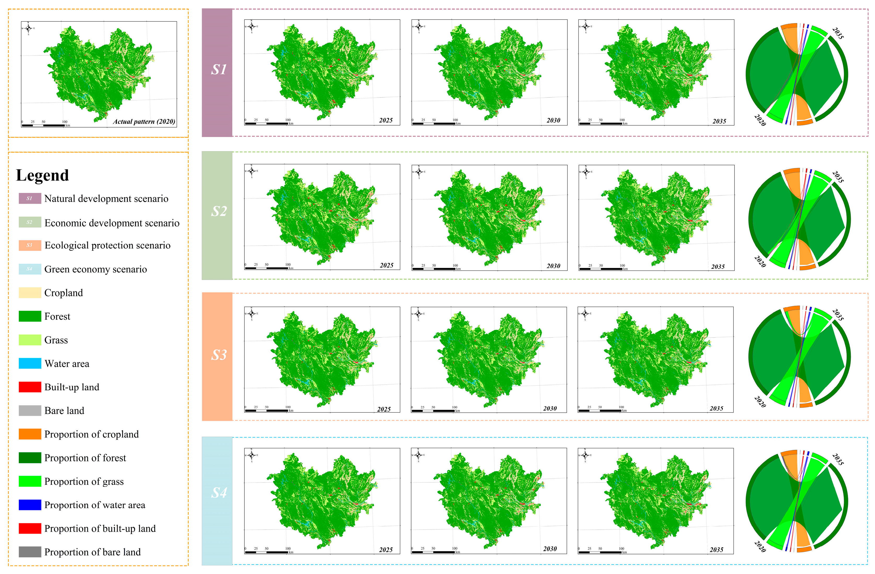
4.3. Predicting Different LUCCs in Multiple Scenarios

4.3.1. Spatial Changes in Land Use Types

Figure 7 illustrates the anticipated alterations in land use types between 2020 and 2035 in Hechi City, as projected under four distinct scenarios: the NDS, EDS, EPS, and GES. The distribution of cropland is concentrated in the eastern region, with the remainder distributed throughout Hechi. Among these, the cropland in the EPS scenario decreased from 2020 to 2025, with the greatest decline occurring in the eastern region. The forest area is the largest, with the majority distributed in high-altitude areas, including the western, southern, and northern regions of Hechi City. Grass is mainly distributed in the northeast and northwest. The water area is primarily situated in the western and southwestern regions of Hechi City. Between the years 2020 and 2035, the EPS scenario exhibited the most pronounced increase in water area, with the majority of this expansion occurring in the vicinity of rivers in the eastern region. The distribution of built-up land is concentrated in the central and eastern regions of Hechi City, with the majority of this land situated in areas of low elevation. Among the four scenarios, the expansion area of built-up land under the NDS, EDS, and EPS is relatively uniform, mainly around the original built-up area. In contrast, in GES, the main areas of construction land expansion in Hechi City are located in the northeast, east and south. The range of the change of bare land is relatively limited across all scenarios. By 2035, the EDS will have the largest cropland area and built-up land area, which will be 39.60 × 10⁴ hm² and 2.92 × 10⁴ hm², respectively. The EPS will have the largest forest area and grassland area, which will be 249.80 × 10⁴ hm² and 47.32 × 10⁴ hm², respectively. The GES is a harmonious scenario between the EDS and EPS, and its built-up land area will be the same as that of the EDS. The NDS will have the most bare land. Its cropland area will be 38.98 × 10⁴ hm², which will be similar to that of the EDS, and its grassland area will be 42.04 × 10⁴ hm², which will be consistent with that of the GES.

4.3.2. Temporal Changes in Land Use Types

From 2020 to 2035, the cropland area in the NDS, EPS, and GES will decrease from 39.25 × 10⁴ hm² to 38.98 × 10⁴ hm², 31.44 × 10⁴ hm², and 35.77 × 10⁴ hm², respectively (Figure 8). This trend will mainly be due to the implementation of the policy of returning farmland to forests. The area of EPS cropland will significantly decrease by 19.89%. One reason for this result is that the scenario prioritizes high ecological value, while cropland has relatively low ecological value. As a result, the area of cropland will be reduced. In contrast, the cropland area of the EDS will increase to 39.60 × 10⁴ hm² in 2035. This result is mainly due to the high economic value provided by crops, which aligns with the development goal of this scenario. The forest area will show a slightly decreasing, decreasing, increasing and increasing trend in the four scenarios, from 248.53 × 10⁴ hm² in 2020 to 247.76 × 10⁴ hm², 242.94 × 10⁴ hm², 249.80 × 10⁴ hm² and 249.80 × 10⁴ hm² in 2035. The grassland area will show a slightly increasing, increasing, increasing and decreasing trend, from 42.03 × 10⁴ hm² in 2020 to 42.04 × 10⁴ hm², 45.68 × 10⁴ hm², 47.32 × 10⁴ hm² and 42.04 × 10⁴ hm² in 2035. The water area will show an increasing trend in the four scenarios, among which the EPS will increase the most, from 3.08 × 10⁴ hm² in 2020 to 4.25 × 10⁴ hm² in 2035. The built-up land area will increase in all four scenarios, with growth rates of 30.04%, 56.09%, 4.06% and 56.09%. Among them, the EPS will have the slowest growth rate, at only 4.06%. The bare land area will decrease in all scenarios.

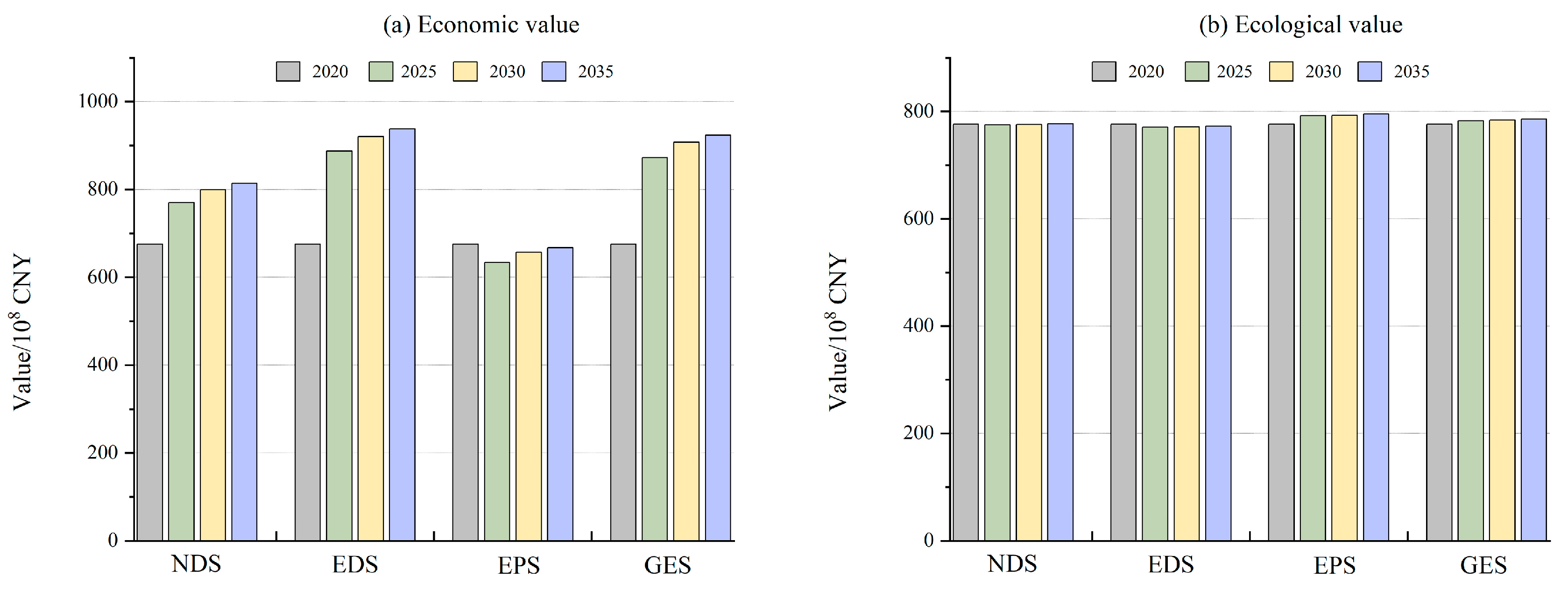
4.4. Evaluation of Ecological and Economic Value under Different Scenarios

Within the scenario of gaining economic value from 2020 to 2035, the EPS and GES will show rapid growth, while the NDS and EDS will increase slowly (Figure 9). Among these four scenarios, the economic value provided by the EDS will be the highest, reaching CNY 938.01 × 10⁸, followed by that provided by the GES, which will be CNY 924.08 × 10⁸. The economic value provided by the EPS will be the lowest, at only CNY 667.46 × 10⁸. The main reason for the significant difference in economic value among the four scenarios is the difference in their future built-up land area. Among the scenarios, the EPS will have the least amount of construction land; therefore, it will have the lowest economic value. Considering the future development of the city, the EPS will have a lower economic value than the other scenarios, which will not be in line with the urban development plan. Therefore, the possibility of its future development, according to this scenario, is relatively small. In 2035, among the ecological values provided by the various scenarios, the EPS will have the highest value, reaching CNY 794.98 × 10⁸, followed by the GES, at CNY 785.62 × 10⁸. In 2035, the ecological values of the NDS, EPS and GES will all increase, but that of the EDS will decrease to CNY 3.40 × 10⁸ lower than that in 2020. The main reason for this decline will be the loss of ecological value of the EDS from 2020 to 2025, while the loss of ecological value will mainly be caused by the degradation of forests and cropland, with a total loss of CNY 5.31 × 10⁸ during this period.

The study suggests that the GES may be the most suitable scenario for local development, as the NDS does not offer any significant advantages in terms of economic or ecological value compared to the other scenarios. Although the EDS provides the highest economic value, it is estimated that its ecological value will be CNY 772.57 × 10⁸ by 2035, which is the least of all the scenarios. And the ecological value of this scenario is expected to decrease from 2020 to 2025. While the EPS has the highest ecological value, its economic value is too low. On the other hand, the GES will have a slightly lower economic value than the EDS, 13.93 × 10⁸ CNY lower in 2035, but it will be significantly greater than that of the NDS and EPS. The ecological value of the GES is equivalent to that of EPS, and its future ecological value will also increase. There will be no retrogression of these two values in the future. Therefore, prioritizing the development of the GES, which provides relatively high ecological and economic value, is more reasonable in future regional planning, and it has the best effect.

5. Discussion

5.1. Feasibility of the Research Frame

The study predicted the dynamic quantity and space distribution of six land use types in the future, which can provide strong support for sustainable regional development [45,46]. This study makes two main contributions: the in-depth analysis of the driving forces of land use change based on the PLUS model, and the selection of optimal future scenarios under the influence of government policies.

First, this study demonstrates accurate and effective characteristics by modeling land use types. Markov chains can simulate future land quantities using two-period land use data, which means that this method has a unique advantage in the cases of limited data. But social and economic factors are not taken into account, and combining it with the MOP method makes up for this shortcoming [47]. In addition to the PLUS model, the FLUS and CLUE-S models are commonly used for land use prediction [48,49]. Compared to these two models, the PLUS model not only obtains high accuracy in the simulation process but also demonstrates a landscape pattern that is more consistent with reality [23]. The significance of the variables obtained from the PLUS model reveals a number of previously undiscovered processes of land use change. For instance, elevation made a relatively high contribution to each of the six land-use change categories, suggesting that elevation represents a significant factor influencing land use change within the region. Deciduous forests are likely to grow along main or secondary roads in suburban areas, while grasslands are likely to grow in areas with few impacts from human activity. These findings can help policymakers understand how drivers influence short-term land use change.

Second, to design future optimal scenarios under the influence of policies, we use the MOP approach to calculate the corresponding land demand area. In traditional approaches, simple land use projections are usually made through Markov chains [50], or SD models are used after considering social, economic, and climatic factors in the study area [10,51]. However, in our chosen study area, government plans and policies have a greater impact on the development of future regional areas, making these approaches slightly insufficient. In our research, based on government policies and other socioeconomic factors, we designed three scenarios, the EDS, EPS and GES, by maximizing the ecological or economic value under the established policies and integrating them into the PLUS model to produce good simulation results. The goal was to achieve optimal spatial distributions and area requirements that are more closely related to the possible future development of Hechi City [52]. In setting the optimal scenarios, this paper improves upon the studies of other scholars. Liang et al. [20] calculated the values of balanced scenarios by summing the economic and ecological values, but the difference between the two values was so large that the difference in value between the scenarios was too large, which was not conducive to scenario comparison. Peng et al. [12] adjusted the value of balanced scenarios by setting the weights in their study, but the weights were based on the ratio between the economic value coefficients and the ecological value coefficients. In this paper, for the setting of the GES of the best scenario, we adjust the allocation of weights by setting the step size to ensure that the GES is set reasonably and accurately. This method has the advantage of ensuring that there is a gap in value between scenarios but that it is not too large, which is conducive to making comparisons between scenarios.

5.2. Potential Contribution to Local Policies

The implementation of the GDAP is conducive to driving the construction of local areas for a strong ecological civilization. The utilization of land resources is essential in all fields of work. Within what range will future regional planning be reasonable? This paper provides a reference suggestion. We calculated the environmental and economic values of each scenario, to weigh the ecological and economic values between different scenes. Although the ecological and economic values of the GES are not the highest among the four scenarios, their land ecological values and economic values are more balanced than those of the other scenarios. Moreover, the ecological and economic values are the second highest of all scenarios, which is in line with the original intent of the GDAP, that is, developing the economy without causing harm to the environment. For future planning suggestions, we expect that the cropland area will decrease in the future and the altitude has the greatest influence on the cropland growth. Therefore, in the future, the inferior cropland in high-altitude areas should be reduced and converted to other land uses. The area of grass exhibited little change in the GES and NDS, but showed a rising trend in the EDS and EPS. The local government should pay special attention to the protection and restoration of grass in key ecological areas. Water area can provide high ecosystem service value, and its area will increase in the future. The protection of rivers, wetlands and other water areas should be strengthened to ensure the ecological safety of water sources. In urban construction, it is necessary to strictly observe the urban development boundary, attach importance to the secondary development of restricted and abandoned construction land, and carry out new urbanization construction centered on county towns. Generally speaking, the research results can help policymakers understand the trade-offs and synergies between economic development and ecological protection, and guide the formulation of future land use plans.

5.3. Limitations

The choice of driving factors is subjective and is based on a literature review and personal understanding. Whether or not there are factors that have not been considered, is not explained in this study. Additionally, the classification of land use types is not detailed enough, which could impact subsequent value calculations. For example, a change in cultivated land will affect the change in forestland types, thus affecting the economic value of forestland [53]. Additionally, our spatial allocation model still has certain shortcomings. First, the MOP algorithm does not consider economic constraints. Our constraints are mainly based on land use policies and historical trends, and we ignore the impact of human activities on these trends, thus reducing the estimation accuracy of demand areas. Moreover, in our PLUS model, the local government has planned an ecological protection area, but because the data have not been made public, the restricted development area which is set is smaller than the actual area, which may lead to problems in the simulation results.

6. Conclusions

This study projected land use patterns for the period 2020-2035 and assessed land values to determine the most applicable scenarios for policies in the region. The specific conclusions are presented below:

(1) The study analyzed the potential drivers of land use change and revealed differences in their influence on various land use types. However, elevation was found to strongly influence all six land use types.

(2) Compared with those in 2020, the land value assessment results indicate an increase in the sum of the economic and ecological values in all scenarios. While both the EDS and GES provide higher ecological and economic values, the EDS shows a decrease in ecological values from 2020 to 2025.

(3) The “optimal scenario” should be policy compliance; that is, the best scheme must comply with the principles and regulations outlined in GDAP. In addition, economic feasibility, sustainable utilization of natural resources, and maintenance of ecosystem services should be considered, and it should have the potential to expand to a regional or national level. All four scenarios are possible in the future. However, the GES is more aligned with the GDAP because it implements the ‘green development concept’ and acquires significant land value.

References

1. Chhabra, A.; Geist, H.; Houghton, R.A.; Haberl, H.; Braimoh, A.K.; Vlek, P.L.; Patz, J.; Xu, J.; Ramankutty, N.; Coomes, O. Multiple impacts of land-use/cover change. In Land-Use and Land-Cover Change: Local Processes and Global Impacts; Springer: Berlin/Heidelberg, Germany, 2006; pp. 71–116. [Google Scholar]
2. Liu, J.; Diamond, J. China’s environment in a globalizing world. Nature 2005, 435, 1179–1186. [Google Scholar] [CrossRef]
3. Zhou, X.; Kang, C. Land use/cover change analysis in Wuhan city based on RS and GIS. In Proceedings of the 2011 19th International Conference on Geoinformatics, Shanghai, China, 24–26 June 2011; pp. 1–5. [Google Scholar]
4. UN. Transforming Our World: The 2030 Agenda for Sustainable Development; United Nations: New York, NY, USA, 2015. [Google Scholar]
5. Ma, T.T.; Li, X.; Bai, J.; Cui, B. Tracking three decades of land use and land cover transformation trajectories in China’s large river deltas. Land Degrad. Dev. 2019, 30, 799–810. [Google Scholar] [CrossRef]
6. Peng, L.; Tang, C.; Zhang, X.; Duan, J.; Yang, L.; Liu, S. Quantifying the effects of root and soil properties on soil detachment capacity in agricultural land use of Southern China. Forests 2022, 13, 1788. [Google Scholar] [CrossRef]
7. Zhu, Y. Policy Entrepreneur, Civic Engagement and Local Policy Innovation in China: Housing Monetarisation Reform in Guizhou Province. Aust. J. Public Adm. 2012, 71, 191–200. [Google Scholar] [CrossRef]
8. Li, C.; Wu, Y.; Gao, B.; Zheng, K.; Wu, Y.; Li, C. Multi-scenario simulation of ecosystem service value for optimization of land use in the Sichuan-Yunnan ecological barrier, China. Ecol. Indic. 2021, 132, 108328. [Google Scholar] [CrossRef]
9. Wang, Y.; Li, X.; Zhang, Q.; Li, J.; Zhou, X. Projections of future land use changes: Multiple scenarios-based impacts analysis on ecosystem services for Wuhan city, China. Ecol. Indic. 2018, 94, 430–445. [Google Scholar] [CrossRef]
10. Wu, J.; Luo, J.; Zhang, H.; Qin, S.; Yu, M. Projections of land use change and habitat quality assessment by coupling climate change and development patterns. Sci. Total Environ. 2022, 847, 157491. [Google Scholar] [CrossRef] [PubMed]
11. Hu, S.; Chen, L.; Li, L.; Zhang, T.; Yuan, L.; Cheng, L.; Wang, J.; Wen, M. Simulation of land use change and ecosystem service value dynamics under ecological constraints in Anhui Province, China. Int. J. Environ. Res. Public Health 2020, 17, 4228. [Google Scholar] [CrossRef]
12. Peng, K.; Jiang, W.; Wang, X.; Hou, P.; Wu, Z.; Cui, T. Evaluation of future wetland changes under optimal scenarios and land degradation neutrality analysis in the Guangdong-Hong Kong-Macao Greater Bay Area. Sci. Total Environ. 2023, 879, 163111. [Google Scholar] [CrossRef]
13. Zhu, W.; Jiang, Z.; Cen, L.; Wu, H. Evaluation, simulation, and optimization of land use spatial patterns for high-quality development: A case study of Zhengzhou city, China. J. Geogr. Sci. 2023, 33, 266–288. [Google Scholar] [CrossRef]
14. Wu, H.; Lin, A.; Xing, X.; Song, D.; Li, Y. Identifying core driving factors of urban land use change from global land cover products and POI data using the random forest method. Int. J. Appl. Earth Obs. Geoinf. 2021, 103, 102475. [Google Scholar] [CrossRef]
15. Zhou, L.; Dang, X.; Sun, Q.; Wang, S. Multi-scenario simulation of urban land change in Shanghai by random forest and CA-Markov model. Sustain. Cities Soc. 2020, 55, 102045. [Google Scholar] [CrossRef]
16. Rahnama, M.R. Forecasting land-use changes in Mashhad Metropolitan area using Cellular Automata and Markov chain model for 2016–2030. Sustain. Cities Soc. 2021, 64, 102548. [Google Scholar] [CrossRef]
17. Tan, J.; Li, A.; Lei, G.; Xie, X. A SD-MaxEnt-CA model for simulating the landscape dynamic of natural ecosystem by considering socio-economic and natural impacts. Ecol. Model. 2019, 410, 108783. [Google Scholar] [CrossRef]
18. Chang, Y.-C.; Ko, T.-T. An interactive dynamic multi-objective programming model to support better land use planning. Land Use Policy 2014, 36, 13–22. [Google Scholar] [CrossRef]
19. Zhao, C.; Zhou, Y.; Lai, X. An integrated framework with evolutionary algorithm for multi-scenario multi-objective optimization problems. Inf. Sci. 2022, 600, 342–361. [Google Scholar] [CrossRef]
20. Liang, X.; Liu, X.; Li, D.; Zhao, H.; Chen, G. Urban growth simulation by incorporating planning policies into a CA-based future land-use simulation model. Int. J. Geogr. Inf. Sci. 2018, 32, 2294–2316. [Google Scholar] [CrossRef]
21. Huang, D.; Huang, J.; Liu, T. Delimiting urban growth boundaries using the CLUE-S model with village administrative boundaries. Land Use Policy 2019, 82, 422–435. [Google Scholar] [CrossRef]
22. Wang, S.; Zheng, X. Dominant transition probability: Combining CA-Markov model to simulate land use change. Environ. Dev. Sustain. 2023, 25, 6829–6847. [Google Scholar] [CrossRef]
23. Liang, X.; Guan, Q.; Clarke, K.C.; Liu, S.; Wang, B.; Yao, Y. Understanding the drivers of sustainable land expansion using a patch-generating land use simulation (PLUS) model: A case study in Wuhan, China. Comput. Environ. Urban Syst. 2021, 85, 101569. [Google Scholar] [CrossRef]
24. Luan, C.; Liu, R. A comparative study of various land use and land cover change models to predict ecosystem service value. Int. J. Environ. Res. Public Health 2022, 19, 16484. [Google Scholar] [CrossRef]
25. Zhang, Y.; Chang, X.; Liu, Y.; Lu, Y.; Wang, Y.; Liu, Y. Urban expansion simulation under constraint of multiple ecosystem services (MESs) based on cellular automata (CA)-Markov model: Scenario analysis and policy implications. Land Use Policy 2021, 108, 105667. [Google Scholar] [CrossRef]
26. Zhang, Z.; Hu, B.; Jiang, W.; Qiu, H. Spatial and temporal variation and prediction of ecological carrying capacity based on machine learning and PLUS model. Ecol. Indic. 2023, 154, 110611. [Google Scholar] [CrossRef]
27. Yang, Y.; Wang, H.; Li, X.; Huang, X.; Lyu, X.; Tian, H.; Qu, T. How will ecosystem carbon sequestration contribute to the reduction of regional carbon emissions in the future? analysis based on the MOP-PLUS model framework. Ecol. Indic. 2023, 156, 111156. [Google Scholar] [CrossRef]
28. Aung, T.S.; Fischer, T.B.; Buchanan, J. Land use and land cover changes along the China-Myanmar Oil and Gas pipelines–Monitoring infrastructure development in remote conflict-prone regions. PLoS ONE 2020, 15, e0237806. [Google Scholar] [CrossRef] [PubMed]
29. Shafizadeh-Moghadam, H.; Minaei, M.; Pontius Jr, R.G.; Asghari, A.; Dadashpoor, H. Integrating a forward feature selection algorithm, random forest, and cellular automata to extrapolate urban growth in the Tehran-Karaj Region of Iran. Comput. Environ. Urban Syst. 2021, 87, 101595. [Google Scholar] [CrossRef]
30. Li, X.; Fu, J.; Jiang, D.; Lin, G.; Cao, C. Land use optimization in Ningbo City with a coupled GA and PLUS model. J. Clean. Prod. 2022, 375, 134004. [Google Scholar] [CrossRef]
31. Lin, X.; Jiao, X.; Tian, Z.; Sun, Q.; Zhang, Y.; Zhang, P.; Ji, Z.; Chen, L.; Lun, F.; Chang, X. Projecting diversity conflicts of future land system pathways in China under anthropogenic and climate forcing. Earth’s Future 2023, 11, e2022EF003406. [Google Scholar] [CrossRef]
32. Yang, S.; Su, H.; Zhao, G. Multi-scenario simulation of urban ecosystem service value based on PLUS model: A case study of Hanzhong city. J. Arid. Land. Res. Env. 2022, 36, 86–95. [Google Scholar]
33. Hu, Y.; Batunacun; Zhen, L.; Zhuang, D. Assessment of land-use and land-cover change in Guangxi, China. Sci. Rep. 2019, 9, 2189. [Google Scholar] [CrossRef]
34. Zhang, T.; Cheng, C.; Wu, X. Mapping the spatial heterogeneity of global land use and land cover from 2020 to 2100 at a 1 km resolution. Sci. Data 2023, 10, 748. [Google Scholar] [CrossRef] [PubMed]
35. Lin, J.; He, P.; Yang, L.; He, X.; Lu, S.; Liu, D. Predicting future urban waterlogging-prone areas by coupling the maximum entropy and FLUS model. Sustain. Cities Soc. 2022, 80, 103812. [Google Scholar] [CrossRef]
36. Bu, R.; Chang, Y.; Hu, Y.; Li, X.; He, H. Measuring spatial information changes using Kappa coefficients: A case study of the city groups in central Liaoning province. Acta Ecol. Sin. 2005, 25, 778–784. [Google Scholar]
37. Zhang, S.; Yang, P.; Xia, J.; Wang, W.; Cai, W.; Chen, N.; Hu, S.; Luo, X.; Li, J.; Zhan, C. Land use/land cover prediction and analysis of the middle reaches of the Yangtze River under different scenarios. Sci. Total Environ. 2022, 833, 155238. [Google Scholar] [CrossRef] [PubMed]
38. Gardiner, L.R.; Steuer, R.E. Unified interactive multiple objective programming. Eur. J. Oper. Res. 1994, 74, 391–406. [Google Scholar] [CrossRef]
39. Peng, K.; Jiang, W.; Deng, Y.; Liu, Y.; Wu, Z.; Chen, Z. Simulating wetland changes under different scenarios based on integrating the random forest and CLUE-S models: A case study of Wuhan Urban Agglomeration. Ecol. Indic. 2020, 117, 106671. [Google Scholar] [CrossRef]
40. Xie, G.; Zhang, C.-X.; Zhang, L.-M.; Chen, W.; Li, S. Improvement of the evaluation method for ecosystem service value based on per unit area. J. Nat. Resour. 2015, 30, 1243. [Google Scholar]
41. Gao, M.; Hu, Y.; Bai, Y. Construction of ecological security pattern in national land space from the perspective of the community of life in mountain, water, forest, field, lake and grass: A case study in Guangxi Hechi, China. Ecol. Indic. 2022, 139, 108867. [Google Scholar] [CrossRef]
42. Li, C.; Su, K.; Liang, X.; Jiang, X.; Wang, J.; You, Y.; Wang, L.; Chang, S.; Wei, C.; Zhang, Y. Identification of priority areas to provide insights for ecological protection planning: A case study in Hechi, China. Ecol. Indic. 2023, 154, 110738. [Google Scholar] [CrossRef]
43. Long, Y.; Han, H.; Lai, S.-K.; Mao, Q. Urban growth boundaries of the Beijing Metropolitan Area: Comparison of simulation and artwork. Cities 2013, 31, 337–348. [Google Scholar] [CrossRef]
44. UNEP-WCMC; IUCN. Protected Planet: The World Database on Protected Areas (WDPA); UNEP-WCMC: Cambridge, UK; IUCN: Cambridge, UK, 2020. [Google Scholar]
45. Schillaci, C.; Jones, A.; Vieira, D.; Munafò, M.; Montanarella, L. Evaluation of the United Nations Sustainable Development Goal 15.3.1 indicator of land degradation in the European Union. Land Degrad. Dev. 2023, 34, 250–268. [Google Scholar] [CrossRef]
46. Tian, P.; Cao, L.; Li, J.; Pu, R.; Gong, H.; Li, C. Landscape characteristics and ecological risk assessment based on multi-scenario simulations: A case study of Yancheng Coastal Wetland, China. Sustainability 2020, 13, 149. [Google Scholar] [CrossRef]
47. Zhang, D.; Liu, X.; Wu, X.; Yao, Y.; Wu, X.; Chen, Y. Multiple intra-urban land use simulations and driving factors analysis: A case study in Huicheng, China. GIScience Remote Sens. 2019, 56, 282–308. [Google Scholar] [CrossRef]
48. Liu, X.; Liang, X.; Li, X.; Xu, X.; Ou, J.; Chen, Y.; Li, S.; Wang, S.; Pei, F. A future land use simulation model (FLUS) for simulating multiple land use scenarios by coupling human and natural effects. Landsc. Urban Plan. 2017, 168, 94–116. [Google Scholar] [CrossRef]
49. Wu, M.; Ren, X.; Che, Y.; Yang, K. A coupled SD and CLUE-S model for exploring the impact of land use change on ecosystem service value: A case study in Baoshan District, Shanghai, China. Environ. Manag. 2015, 56, 402–419. [Google Scholar] [CrossRef] [PubMed]
50. Xiao, Y.; Huang, M.; Xie, G.; Zhen, L. Evaluating the impacts of land use change on ecosystem service values under multiple scenarios in the Hunshandake region of China. Sci. Total Environ. 2022, 850, 158067. [Google Scholar] [CrossRef] [PubMed]
51. Ji, X.; Sun, Y.; Guo, W.; Zhao, C.; Li, K. Land use and habitat quality change in the Yellow River Basin: A perspective with different CMIP6-based scenarios and multiple scales. J. Environ. Manag. 2023, 345, 118729. [Google Scholar] [CrossRef] [PubMed]
52. Xu, L.; Liu, X.; Tong, D.; Liu, Z.; Yin, L.; Zheng, W. Forecasting urban land use change based on cellular automata and the PLUS model. Land 2022, 11, 652. [Google Scholar] [CrossRef]
53. Diniz, M.F.; Coelho, M.T.P.; Sánchez-Cuervo, A.M.; Loyola, R. How 30 years of land-use changes have affected habitat suitability and connectivity for Atlantic Forest species. Biol. Conserv. 2022, 274, 109737. [Google Scholar] [CrossRef]
Figure 1. Workflow of land use-change modeling.
Sustainability 16 05039 g001
Figure 2. Land use-change conversion diagram.
Sustainability 16 05039 g002
Figure 3. Land use-distribution map of Hechi City in 2020.
Sustainability 16 05039 g003
Figure 4. Land use changes in Hechi City, 1990–2020 (only the amount of land that underwent transformation is shown).
Sustainability 16 05039 g004
Figure 5. The expansion areas of land use types overlap with the most important driving factors.
Sustainability 16 05039 g005
Figure 6. The importance of the contribution of all driving factors to land growth.
Sustainability 16 05039 g006
Figure 7. Land use under multi scenarios in Hechi City from 2020 to 2035.
Sustainability 16 05039 g007
Figure 8. Temporal changes in land use types in Hechi, 2020–2035.
Sustainability 16 05039 g008
Figure 9. Economic and ecological values under the different scenarios, 2020–2035.
Sustainability 16 05039 g009