Spatial Patterns and Determinants of PM_2.5 Concentrations: A Land Use Regression Analysis in Shenyang Metropolitan Area, China

Abstract

Identifying impact factors and spatial variability of pollutants is essential for understanding environmental exposure and devising solutions. This research focused on PM_2.5 as the target pollutant and developed land use regression models specific to the Shenyang metropolitan area in 2020. Utilizing the Least Absolute Shrinkage and Selection Operator approach, models were developed for all seasons and for the annual average, explaining 62–70% of the variability in PM_2.5 concentrations. Among the predictors, surface pressure exhibited a positive correlation with PM_2.5 concentrations throughout most of the year. Conversely, both elevation and tree cover had negative effects on PM_2.5 levels. At a 2000 m scale, landscape aggregation decreased PM_2.5 levels, while at a larger scale (5000 m), landscape splitting facilitated PM_2.5 dispersion. According to the partial R² results, vegetation-related land use types were significant, with the shrubland proportion positively correlated with local-scale PM_2.5 concentrations in spring. Bare vegetation areas were the primary positive factor in autumn, whereas the mitigating effect of tree cover contrasted with this trend, even in winter. The NDVI, an index used to assess vegetation growth, was not determined to be a primary influencing factor. The findings reaffirm the function of vegetation cover in reducing PM_2.5. Based on the research, actionable strategies for PM_2.5 pollution control were outlined to promote sustainable development in the region.

1. Introduction

PM_2.5, or particulate matter with an aerodynamic diameter of 2.5 micrometers or less, is a hazardous air pollutant comprising a mixture of solid particles and liquid droplets suspended in the atmosphere [1]. Its small size enables it to penetrate deep into the respiratory system upon inhalation, leading to health issues such as asthma, bronchitis, and cardiovascular diseases [2]. The presence of PM_2.5 also leads to environmental degradation through reduced visibility, acid rain formation, and ecosystem damage [3]. The issue of PM_2.5 has become a significant threat to people’s well-being.

The sources of PM_2.5 are diverse, including natural phenomena, such as dust storms, wildfires and sea spray, alongside anthropogenic activities such as the combustion of fossil fuels, and biomass burning [1,4]. PM_2.5 can also form as a secondary pollutant through chemical reactions from primary gaseous emissions [5]. Environmental conditions are also key factors affecting the concentration and distribution of PM_2.5. For instance, meteorological conditions, such as humidity and wind patterns, significantly affect the deposition and dispersion of PM_2.5 particles [6,7]. Geographically, urban centers often exhibit higher PM_2.5 levels compared to rural areas due to higher emission sources from industrial activities and vehicular traffic [8,9]. Topographically, regions situated in valleys or surrounded by mountains may experience reduced air circulation, leading to the accumulation of pollutants and higher PM_2.5 concentrations [10]. Furthermore, land use also influences PM_2.5 levels; for example, areas with dense vegetation tend to have lower concentrations due to the natural air filtration provided by plants [11,12]. More even and scattered landscape distributions were also found to be better for mitigating particulate matter [13]. Shi et al. also found that urban/building morphological parameter was the most decisive factor on street-level air quality in Hong Kong [14]. The identification and quantification of influencing factors are essential for understanding the formation mechanisms and pollution characteristics. However, this task is particularly complex in metropolitan areas or urban agglomerations, where the interplay of multiple factors and their dynamic natures poses significant challenges.

The land use regression (LUR) model is a methodological approach that correlates environmental variables with measured pollutant concentrations to predict air pollution levels at unmonitored locations [15,16]. When the predictors sufficiently capture pollutant concentration variations, the LUR model can operate effectively across various spatial scales. For instance, Hystad et al. utilized site monitoring data to estimate the spatial and temporal characteristics of various pollutants across Canada [17]. Shi et al. focused on predicting NO₂ pollution characteristics at the neighborhood scale along a traffic corridor [18]. Particularly at urban or smaller scales, LUR provides a more efficient and accurate method for estimating ground-level pollution, compared with remote-sensing inversion and air dispersion models [19,20]. This establishes the LUR model as a crucial research tool in fields such as air-quality assessment and exposure assessment in epidemiological studies [21,22]. There are numerous algorithms commonly employed in constructing LUR models, including linear models such as Multiple Linear Regression (MLR), Geographically Weighted Regression (GWR), and Least Absolute Shrinkage and Selection Operator (LASSO), etc. [16]. MLR is the most traditional fitting method in LUR modelling and is widely used [18,23,24]. While the principle is easy to grasp, its capacity to manage complex datasets and account for spatial variations is limited. GWR is a widely used tool for addressing spatial heterogeneity in models by allowing regression coefficients to vary with location [25]. The prerequisite is that it requires a sufficient number of widely distributed observation points for robust results [26,27]. LASSO uses L1 regularization for variable selection and model simplification. It is effective when dealing with a large number of explanatory variables or potential multicollinearity issues [28,29]. Some scholars also use nonlinear algorithms to establish relationships between environmental variables and air quality. GAM captures nonlinear relationships using smoothing functions, making it suitable for data with nonlinear trends [30]. Yet, improper smoothing parameter selection can lead to overfitting, particularly with small data volumes or high noise levels [31]. Machine learning algorithms, such as Random Forest, K-Nearest Neighbor and Support Vector Machine, handle nonlinear relationships effectively, resulting in higher prediction accuracy and being less susceptible to overfitting risks [32]. However, they typically have low interpretability due to “black box” issues [33,34]. Selecting the appropriate algorithm should balance the research problem, data characteristics, and study goals.

A lot of existing studies use the pollutant annual average concentrations from stations or concentrations during designated monitoring periods for modelling and predicting [18,24,35]. These approaches facilitate a comprehensive understanding of the pollution patterns in the study area and allow for the analysis of factors impacting regular or specific pollution events. However, the temporal stability of LUR models, i.e., their ability to accurately predict pollutant patterns across different time periods, has been shown to be limited by studies [36,37]. As previously mentioned, the factors affecting PM_2.5 concentration include both static variables (e.g., land use) and dynamic variables (e.g., meteorological conditions, concentrations of precursor pollutants and vegetation growth changes). Our study sought to determine the consistency of these factors in contributing to seasonal variations in PM_2.5 concentration and to assess whether the pollution patterns of PM_2.5 were stable across different seasons. This helps with the comparison of seasonal disparities in pollution patterns and enhances the understanding of underlying determinants.

Metropolitan areas or urban agglomerations are regions characterized by high population density and intense human activity [38]. These areas exhibit diverse land uses, along with complex spatial patterns. Das et al. developed monthly and annual LUR models to simulate particulate matter concentrations using MLR and LASSO algorithms in the Kolkata Metropolitan Area [37]. Through the comparison, the authors found that the LASSO algorithm’s predictions were superior to those of the MLR; the study focused on the prediction and assessment of pollution exposure, rather than the factors and mechanisms of pollution. Huang et al. examined the impact of land cover on air quality in three major urban areas in China: Jing-Jin-Ji, the Yangtze River Delta, and the Guangdong–Hong Kong–Macau Greater Bay Area. Given that the scale effect was the central focus of the study, land cover was employed as the sole predictor variable category [39]. In this paper, we chose seven cities and one demonstration zone within the Shenyang Metropolitan Area (SYMA) in northeast China. In 2023, it was approved by the National Development and Reform Commission as the ninth national metropolitan area in China and the first in the northeast. Consequently, the research conducted in this area remains very limited, necessitating further investigation. We employed the LASSO method, a machine learning algorithm, to fit the LUR models using data from air-quality monitoring stations. This model established the correlation between PM_2.5 concentrations and multiple source environmental variables, encompassing 34 parameters across 9 categories. Through the identification of key predictor variables, we were able to model the seasonal and yearly PM_2.5 pollution patterns across the study area for the year 2020. The study aims to enhance understanding of the formation mechanisms and pollution characteristics of PM_2.5, particularly in densely populated metropolitan areas with diverse industrial structures and significant environmental stress. By informing the development of targeted control measures, we anticipate that it will make a positive contribution to regional sustainability.

2. Materials and Methods

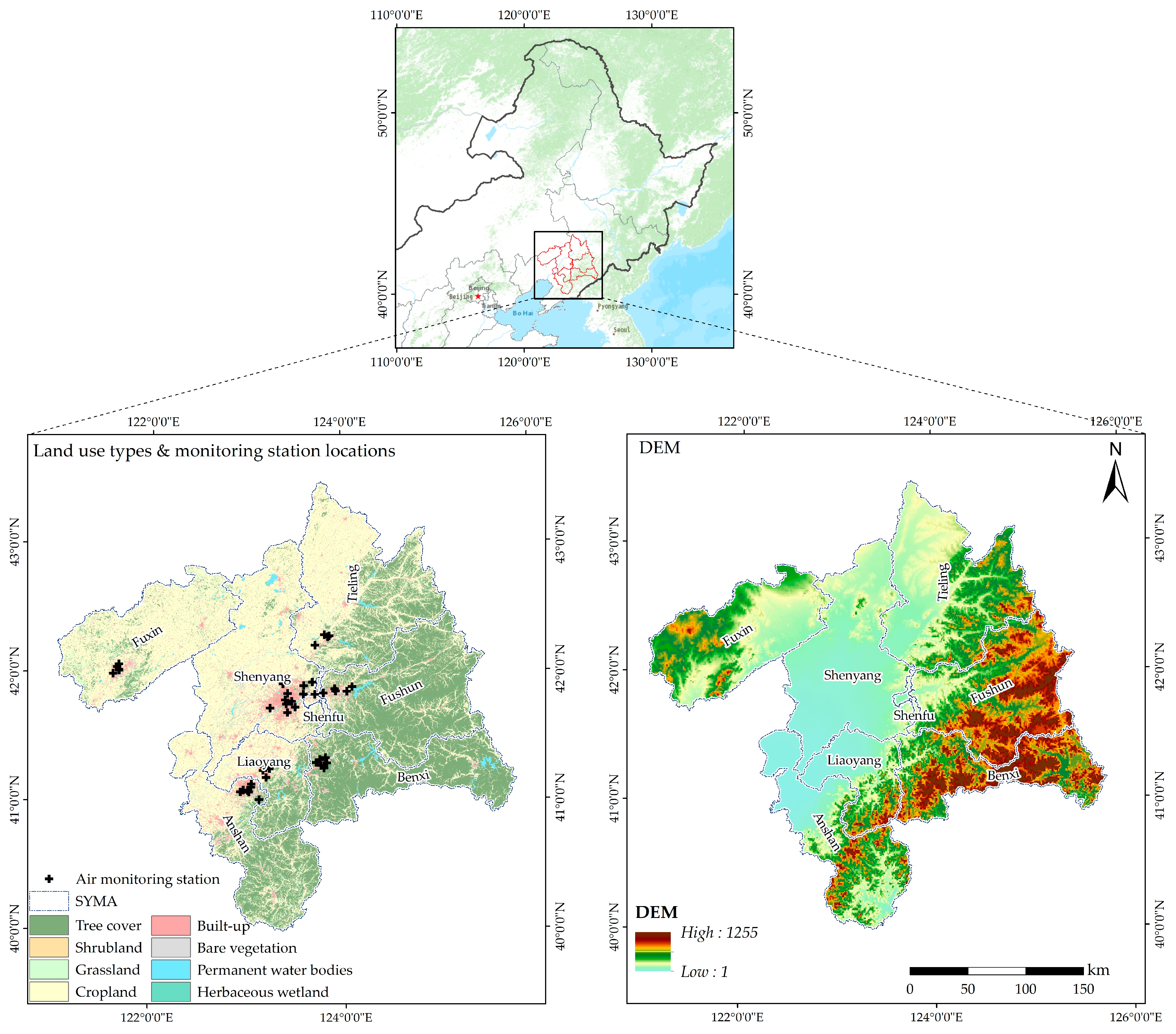
2.1. Study Area

The SYMA is situated in the southern area of Northeast China, within the central part of Liaoning Province. It is centered around the city of Shenyang and encompasses Anshan, Fushun, Benxi, Fuxin, Liaoyang, Tieling and the Shenyang-Fushun (Shenfu) Reform and Innovation Demonstration Zone (Figure 1). The central city, Shenyang, serves as the capital of Liaoning Province and is a significant economic hub in northeast China. The study area experiences a temperate continental monsoon climate, characterized by distinct seasons, with cold and dry winters, hot and rainy summers, and relatively short spring and autumn seasons. The terrain is primarily plains, with some mountainous and hilly areas in the southeast. The hydrology is dominated by the Liao River, with several tributaries, including the Hun River and Taizi River. On the plains, farmland is the predominant land use type, while the mountainous and hilly regions have higher forest coverage. Since the SYMA’s establishment, the GDP has exceeded 1.4 trillion yuan and the population has surpassed 23 million. The primary industries include heavy equipment manufacturing, aerospace, automotive and auto parts sectors, along with services. As a heavy industry hub, the area’s air quality faces certain challenges, making it an appropriate focus for our study.

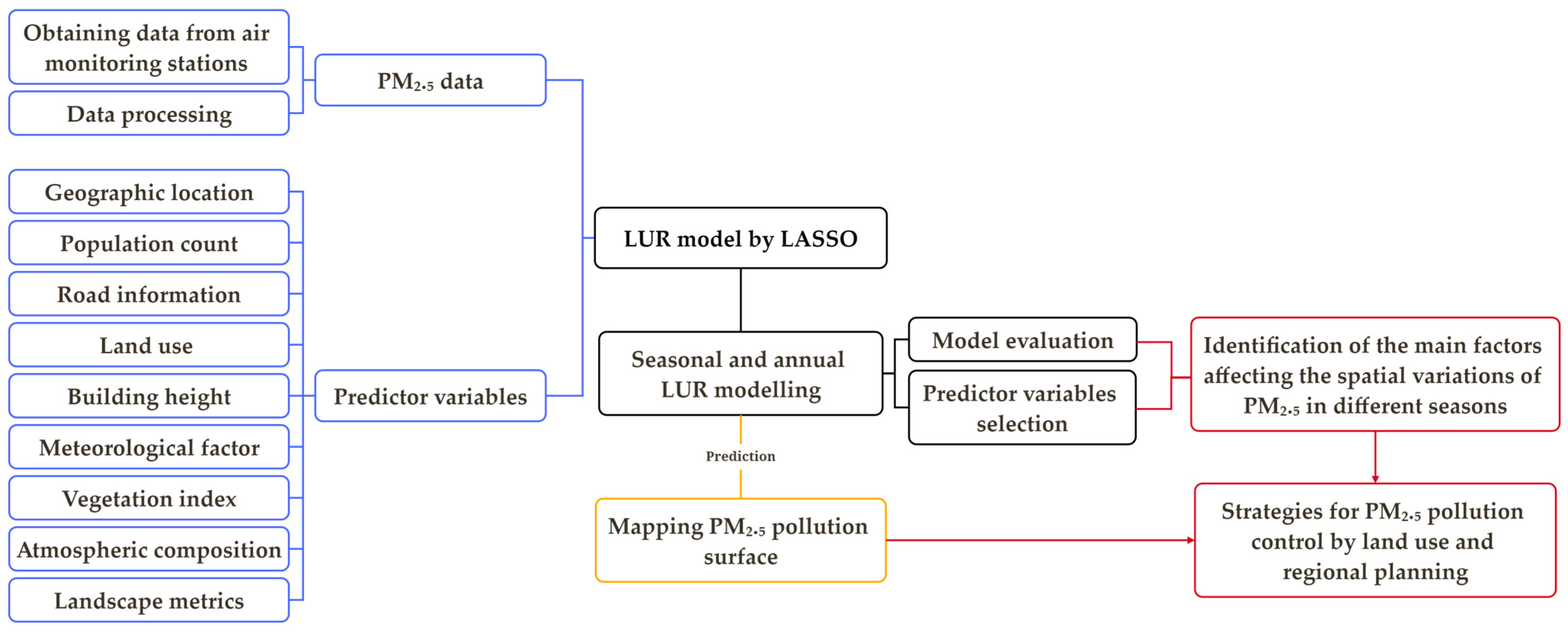
2.2. Technique Route

The workflow is as follows (Figure 2). In the first stage, real-time PM_2.5 data obtained from air-quality monitoring stations were processed, synthesized, and subjected to descriptive statistics to reflect the basic pollution situation in the study area during different seasons and cities. Environmental variables from multiple data sources were also collected and pre-processed to serve as predictors in the subsequent modelling. In the second stage, the LASSO approach was used to select the main variables affecting the spatial variations of PM_2.5, and seasonal and annual LUR models were constructed for subsequent predictions. In the third stage, PM_2.5 pollution maps were generated based on the model results. The seasonal and spatial characteristics of PM_2.5 concentrations were compared and analyzed. Finally, the mechanisms of the main influencing factors were discussed, and insights and strategies for PM_2.5 pollution control were proposed.

2.3. Dependent Variables

PM_2.5 concentration data for SYMA in 2020 were obtained from the Liaoning real-time air-quality publishing system (http://sthj.ln.gov.cn, accessed on 31 December 2020) (Figure 1). Two sites were eliminated owing to a lack of data records and a total of 43 available sites were retained, including 11 monitoring stations in Shenyang, 7 in Ansha, 6 in Benxi, 5 each in Fushun and Fuxin, 4 each in Liaoyang and Tieling, and 1 in Shenfu. The method used to process missing hourly data was as follows: For gaps exceeding 3 h, the average daily variation method was used to estimate the missing values. Specifically, we filled in the mean value of the corresponding time slot from 4 days prior and 4 days after the missing data. For shorter gaps (≤3 h), a linear interpolation method was adopted. The remaining valid data were synthesized to obtain PM_2.5 concentrations during the four seasons (winter: November to March; spring: April to May; summer: June to August; fall: September to October) and for the entire year. The climatic season division was determined based on the national standard (GB/T 42074-2022) and the winter heating period in the study area [24,40,41]. The seasonal and annual means of PM_2.5 concentrations at the monitoring stations were used as dependent variables in the following LUR modelling.

2.4. Predictor Variables

Referring to the index design in Wu et al.’s study [29], combined with the availability of data, nine categories of predictor variables, including 34 parameters, were collected for modelling, based on the influencing factors identified in relevant research findings that directly or potentially contribute to PM_2.5 concentrations (

Table 1. Description of independent variables in land use regression (LUR) modelling.

Category & Variables		Description	Units
Geographic location
1	X	Longitude	°E
2	Y	Latitude	°N
3	DEM	Elevation	m
Population count
4	pop_count	Population count
Road information
5	road_n a	The cumulative road length within a radius of n a m	m
6	dist_road	Distance to the nearest road	m
7	dist_intersection	Distance to the nearest road intersection	m
Land use
8	Tree cover_n a	Proportion of tree cover within radius of n a m	%
9	Shrubland_n a	Proportion of shrubland within radius of n a m	%
10	Grassland_n a	Proportion of grassland within radius of n a m	%
11	Cropland_n a	Proportion of cropland within radius of n a m	%
12	Built-up_n a	Proportion of built-up area within radius of n a m	%
13	Bare vegetation_n a	Proportion of bare vegetation within radius of n a m	%
14	Permanent water bodies_n a	Proportion of permanent water bodies within radius of n a m	%
15	Herbaceous wetland_n a	Proportion of herbaceous wetland within radius of n a m	%
Building height
16	BH_n a	Average building height within radius of n a m	M
Meteorological factors
17	WS	Wind speed	m/s
18	SNSR	Surface net solar radiation	J/m2
19	TEMP	Temperature of air at 2 m	°C
20	RH	Relative humidity	%
21	SP	Pressure of the atmosphere on the surface	Pa
22	LST	Land surface temperature	°C
Vegetation index
23	NDVI	Normalized difference vegetation index
Atmospheric composition
24	AOD	Aerosol optical depth
25	O3_C	Total atmospheric column of O3	mol/m2
26	HCHO_TC	Tropospheric HCHO column number density	mol/m2
27	NO2_TC	Tropospheric vertical column of NO2	mol/m2
Landscape metrics
28	AI_n a	(Aggregation metric) Aggregation index within radius of n a m	%
29	SPLIT_n a	(Aggregation metric) Splitting index within radius of n a m	%
30	IJI_n a	(Aggregation metric) Interspersion and Juxtaposition index within radius of n a m	%
31	FRAC_MN_n a	(Shape metric) Mean fractal dimension index within radius of n a m
32	PAFRAC_n a	(Shape metric) Perimeter-Area fractal dimension within radius of n a m
33	SHDI_n a	(Diversity metric) Shannon’s diversity index within radius of n a m
34	LPI_n a	(Area and Edge metric) Large patch index within radius of n a m

^a n = 50, 100, 200, 500, 1000, 2000, 5000.

) [24,42]. The correlation matrixes detailing the relationships between all independent variables and PM_2.5 concentrations are available in the Supplementary Materials (Figures S1–S5).

Elevation information was derived from the Shuttle Radar Topography Mission digital elevation model Version 4, featuring a spatial resolution of 90 m. The population data were sourced from the LandScan dataset, issued by Oak Ridge National Laboratory, with a spatial resolution of 30 arc-seconds (https://landscan.ornl.gov/, accessed on 20 February 2024). Road data were obtained from Open Street Map (https://www.openstreetmap.org/, accessed on 2 January 2020). Only motorized roads were designated for measuring road lengths. The distances to the nearest road and intersection were computed using the road vector in ArcGIS 10.8. The land use data, with eight land cover classes, were obtained from the European Space Agency World Cover 10 m 2020 product. A description and definition of land cover classes are included in the Supplementary Materials (Section S1 and Table S1). The building heights were derived from CNBH-10 m, a Chinese dataset providing building height information at a resolution of 10 m (https://zenodo.org/records/7923866, accessed on 5 January 2024). The meteorological data, including the 10 m u-component of wind, 10 m v-component of wind, 2 m dewpoint temperature, 2 m temperature, surface pressure (SP) and surface net solar radiation (SNSR), were sourced from daily aggregated data from the fifth-generation ECMWF atmospheric reanalysis of global climate, which has a spatial resolution of 0.25° × 0.25°. The wind speed was calculated based on its u and v components, while the relative humidity was estimated using the rule of thumb based on the dewpoint temperature and the temperature [43]. The daily aggregated data were then averaged seasonally and annually. The data for land surface temperature (LST) were sourced from the MOD11A2 V6.1 product, which offers an 8-day averaged LST within a 1 km grid resolution. The normalized difference vegetation index was obtained from the MOD13A2 V6.1 product, providing vegetation indices within 16 days at 1 km. The 1 km resolution Multi-Angle Implementation of Atmospheric Correction Aerosol Optical Depth, captured by NASA’s Moderate Resolution Imaging Spectroradiometer on the Aqua and Terra satellites, served as a marker for local aerosol conditions. Similarly, imagery for O₃ column number densities (O₃_C), tropospheric nitrogen dioxide (NO₂_TC), and formaldehyde column number density (HCHO_TC) at 1 km resolution was sourced from the Tropospheric Monitoring Instrument on the Sentinel-5P satellite. The majority of the aforementioned data, such as the digital elevation model (DEM), land use data, meteorological data, vegetation index and atmospheric composition, were acquired and processed through the Google Earth Engine platform (https://earthengine.google.com/, accessed on 15 January 2024). With reference to the study by Feng, Liang, and Wu et al. [29,44,45], we selected seven landscape metrics that impact air quality, considering aspects such as aggregation, shape, diversity, and area and edge. A detailed description of the landscape metrics can be found in the Supplementary Materials (Table S2). The landscape metrics were computed based on the land use raster dataset using the “landscapemetrics” package in R [46]. The road length, land use, average building height and landscape metrics were computed by different buffer radii (50, 100, 200, 500, 1000, 2000, 5000 m) at the monitoring stations.

2.5. LUR Modelling and Evaluation

Considering the small sample size and the multiple dimensional predictors in our study’s dataset, along with the approach’s ability to automatically select the most significant influencing variables, we chose the LASSO method to fit the LUR model. The LASSO, a linear regression-based machine learning technique, is noted for improving model interpretability by inducing sparsity. LASSO achieves variable selection and parameter estimation by applying L1 regularization to the regression coefficients. It minimizes a loss function that includes an L1 regularization term, as follows:

$$\mathrm{L}\left(\beta \right)={\sum _{i=1}^n\left(y_i-\sum _{j=1}^p{\beta }_j{x}_{ij}\right)}^2+\lambda \sum _{j=1}^p\left|{\beta }_j\right|$$

(1)

where y_i represents the response variable, x_ij denotes the explanatory variables, β_j are the regression coefficients, n is the number of observations, p is the number of explanatory variables, and λ is the regularization parameter.

The regularization parameter λ controls the strength of the L1 regularization. By increasing λ, LASSO shrinks some regression coefficients to zero, thereby selecting important variables. This process estimates model parameters while automatically selecting significant explanatory variables. The ‘glmnet’ package in R was used to implement the LASSO algorithm [47]. Prior to implementing LASSO, data preprocessing involved normalizing the variables by z-score to mitigate scale-related biases. Normalization ensures that all predictors have a uniform influence on the model, preventing variables with larger ranges from dominating.

To rigorously evaluate the LUR model’s performance, we used leave-one-out cross-validation (LOOCV). In LOOCV, each individual observation in the dataset is sequentially singled out to serve as the sole test instance, with all remaining observations used collectively as the training set. This cycle repeats such that each data point is used exactly once as the test data. This methodical approach ensures a thorough assessment of the model’s performance, as every data point is independently validated against a model trained on all other points. LOOCV is particularly advantageous for small datasets because it maximizes the use of available data for training, thereby reducing bias and allowing for a detailed assessment of the model’s predictive capabilities. To quantitatively measure the model’s predictive performance, we computed evaluation metrics including R-squared (R²) and the root mean squared error (RMSE). These metrics provide a comprehensive view of the model’s ability to generalize across diverse data scenarios by indicating both the proportion of variance explained and the average prediction error, respectively.

Linear regression is predicated on the assumption that residuals are distributed randomly. Deviations from this assumption, such as poor model fits or non-normal distributions of residuals, can arise from several factors, including inappropriate model selection, omission of significant predictors, or the presence of outliers in the dataset. To quantitatively assess the adequacy of our models’ fit, we employed QQ plots to visually inspect the normality of the residuals across various seasonal and average models. Additionally, we conducted Shapiro–Wilk tests to statistically validate the normality assumption of the residuals. QQ plot provide a visual method by plotting the quantiles of the residuals against the quantiles expected under a normal distribution, where alignment along a straight diagonal line indicates normality. The Shapiro–Wilk test offers a quantitative measure of normality; a high p-value (typically greater than 0.05) suggests that the normal distribution model is a good fit to the data.

2.6. Pollution Surface Mapping

The annually averaged and seasonal LUR models were used to generate PM_2.5 concentration maps for the SYMA. Prediction points were created within the study area at a resolution of 1 × 1 km. Using the LUR model outcomes, predictor variables for each point were extracted and multiplied by the corresponding model coefficients. These values were subsequently aggregated and reverse-normalized to ascertain the PM_2.5 concentrations for the respective points. Subsequently, the predicted points were converted into raster format to obtain pollution surface maps using ArcGIS 10.8. Notably, the buffer-related variables were computed based on the buffer values set in the model construction phase. Subsequently, the generated PM_2.5 concentration maps facilitated a comparison of pollution pattern characteristics and disparities across various periods.

3. Results

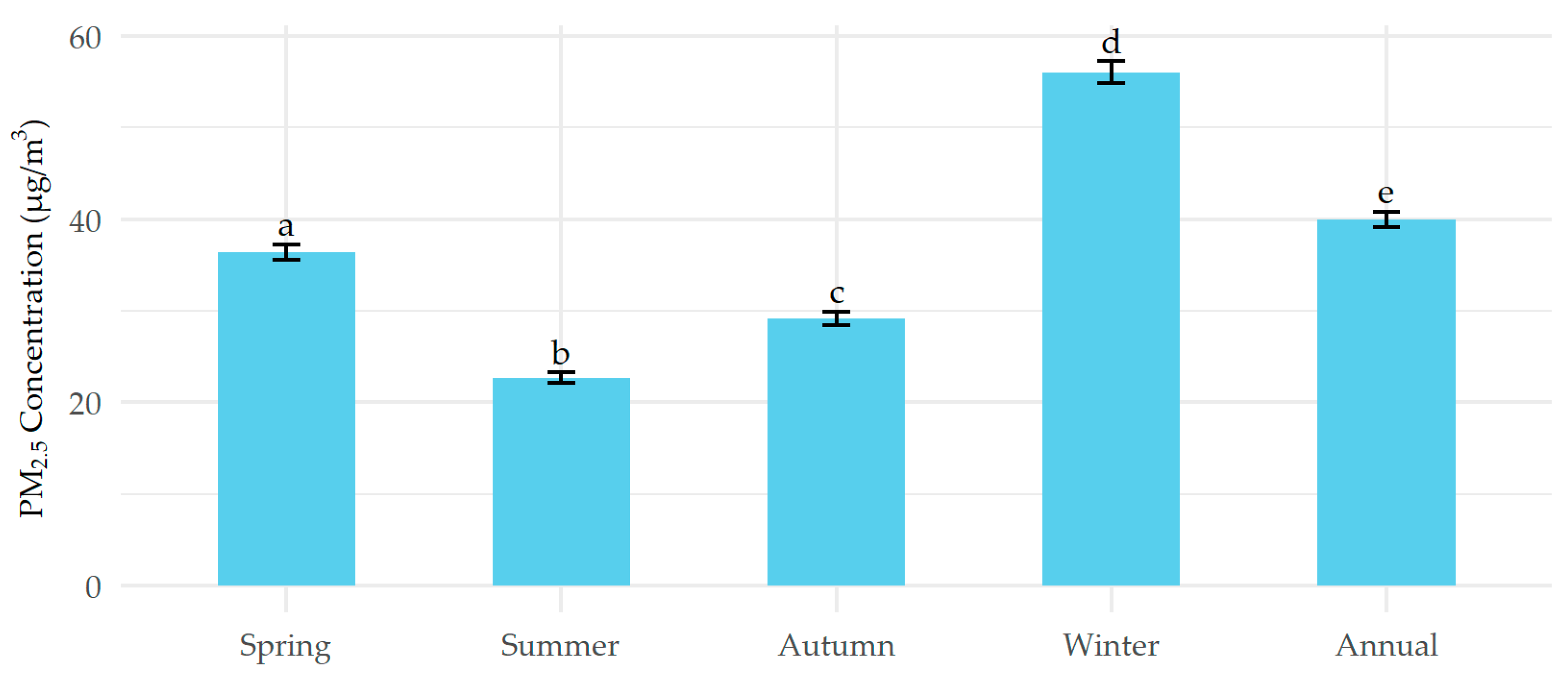
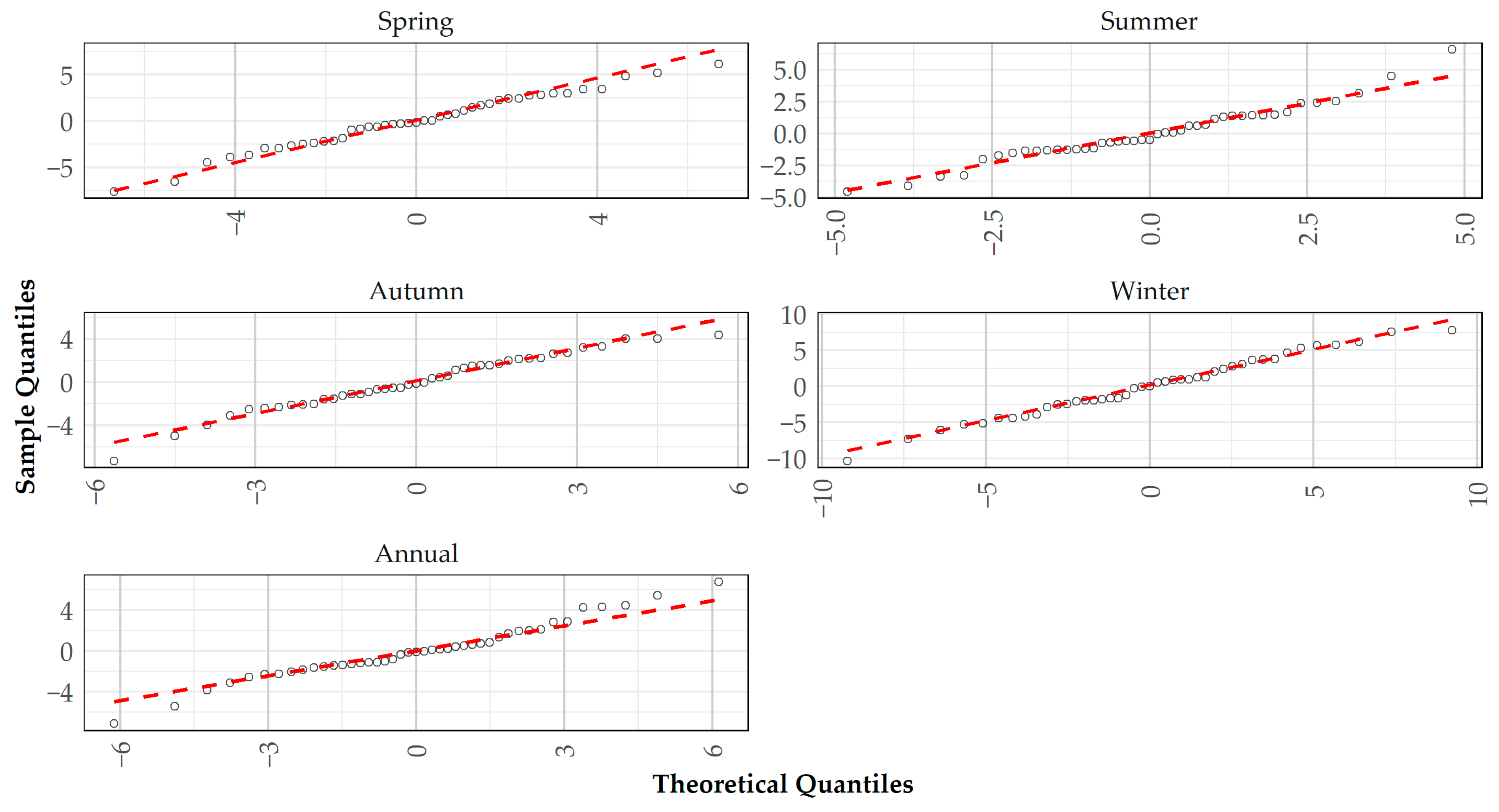
3.1. Descriptive Statistics

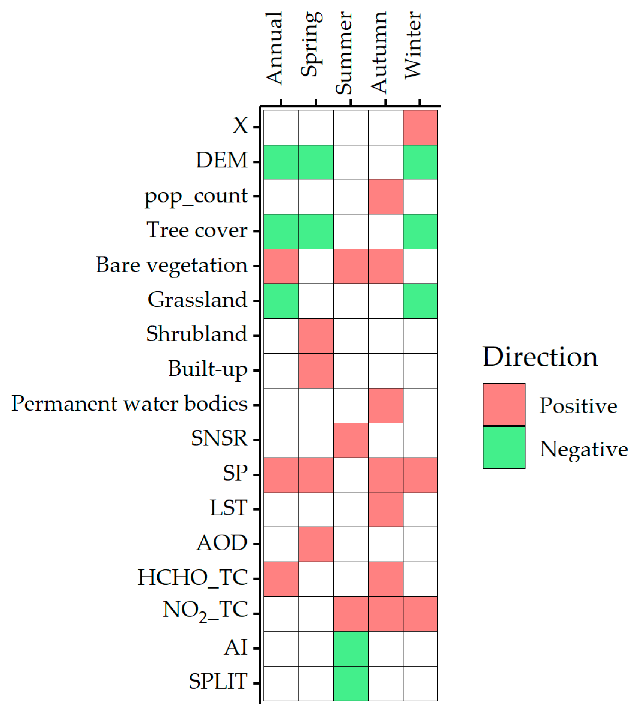
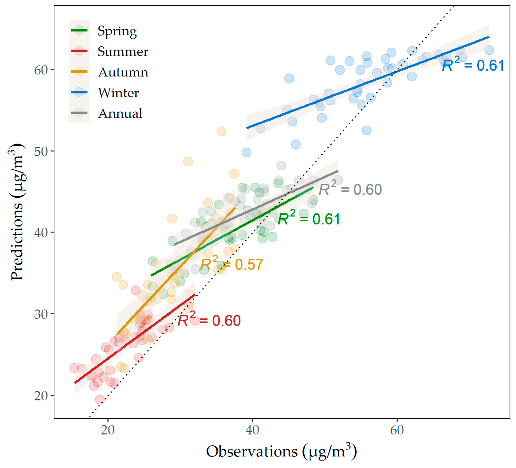
Figure 3 depicts the seasonal variations in PM_2.5 concentrations and Figure 4 shows the variations among different cities and zones within the SYMA. Comprehensive statistical data can be found in the Supplementary Materials (Table S3). PM_2.5 levels showed distinct seasonal fluctuations, peaking in winter, then spring, with the lowest values occurring in summer. At a significance level of p < 0.05, the PM_2.5 concentrations in each season were significantly different from those in all other seasons and the annual period. During winter, concentrations were two to three times higher than those in summer. Despite these seasonal variations, Shenyang, Anshan, Fushun, Liaoyang and Shenfu consistently exhibited higher average and peak PM_2.5 levels compared to the rest of the eight cities/zones analyzed. As shown in Figure 1, the above monitoring stations are concentrated in the plain of the study area.

3.2. LUR Models

The adjusted R² of the annual PM_2.5 LUR model was 0.70, with a range of 0.62–0.69 fitted across the four seasonal models (

Table 2. Summary of the LUR models.

Model	Predictor Variables with Partial R2	adj. R2	LOOCV
			Rcv2	RMSE
Annual	DEM (0.05), Tree cover_500 (0.11), Bare vegetation_5000 (0.18), Grassland_50 (0.17), SP (0.10), HCHO_TC (0.10)	0.70	0.62	3.35
Spring	DEM (0.06), Tree cover_5000 (0.04), Built-up_5000 (0.06), Shrubland_500 (0.08), SP (0.06), AOD (0.01)	0.69	0.65	3.47
Summer	Bare vegetation_5000 (0.17), SNSR (0.27), NO2_TC (0.13), AI_2000 (0.10), SPLIT_5000 (0.17)	0.62	0.56	2.44
Autumn	pop_count (0.07), Bare vegetation_5000 (0.40), Permanent water bodies_2000 (0.13), SP (0.13), LST (0.13), HCHO_TC (0.08), NO2_TC (0.10)	0.69	0.63	3.04
Winter	X (0.04), DEM (0.09), Tree cover_500 (0.29), Grassland_50 (0.15), SP (0.04), NO2_TC (0.01)	0.68	0.61	4.99

Variables with negative coefficient are underlined.

). The LOOCV R² and RMSE values served as indicators of the predictive performance on unseen data. The annual LOOCV R² was 0.62, while the seasonal R² ranged from 0.56 to 0.65. Additionally, the annual RMSE was 3.35 μg/m³, while the seasonal RMSE varied between 2.44 and 4.99 μg/m³. The QQ plots illustrate the distribution of residuals from our model across different seasons and for the entire year. Each plot compares the sample quantiles of residuals against the theoretical quantiles of a standard normal distribution. The close alignment of data points along the dashed red line in each plot indicates a general adherence to normality, with slight deviations observable in the tails (Figure 5). The residuals from the seasonal and annual mean models passed the Shapiro–Wilk test, with p-values greater than 0.05 (spring: p = 0.87; summer: p = 0.20; autumn: p = 0.46; winter: p = 0.93; annual: p = 0.48), further confirming the normality of the residuals. These statistics indicate that the model built is valid and the PM_2.5 concentrations observed were well reproduced.

According to the partial R² values, the contribution of each retained predictor to the model’s fit is identified. The proportion of bare vegetation area within 5000 m (Bare vegetation_5000) and grassland area within 50 m (Grassland_50) explained most of the PM_2.5 concentration variations in the annual model. In the spring model, the 500 m shrubland area ratio (Shrubland_500) had the strongest, albeit low, contribution, with a value of 0.08. In the summer model, SNSR made the strongest contribution. In the autumn model, Bare vegetation_5000 explained most of the variation in PM_2.5 concentrations and in the winter model, the 500 m tree cover area ratio (Tree cover_500) explained the most. Therefore, the distribution of land use related to vegetation had a strong influence on the spatial pattern of PM_2.5 concentrations.

The annual and seasonal LUR models included six categories with 17 variables (Figure 6). SP appeared as an explanatory variable four times, except in the summer model and had a positive effect on PM_2.5 concentration. The DEM, percentage of tree cover and bare vegetation and NO₂_TC appeared three times as predictors in the models. In the models for spring, winter, and annually, both DEM and tree cover negatively impacted PM_2.5 levels. The bare vegetation and NO₂_TC were positively associated with the concentrations. The grassland area ratio in land use types appeared in the annual and winter LUR models with a negative effect, while HCHO_TC appeared in the annual and autumn models with a positive effect on PM_2.5 concentrations.

3.3. PM_2.5 Pollution Surface Mapping

Information on the coefficients of the predictors can be found in the Supplementary Materials (Table S4). Predicted values for the spring, summer, autumn, winter and annual average PM_2.5 pollution surfaces from the LUR models ranged between 22.41 μg/m³ and 58.14 μg/m³, 7.03 μg/m³ and 37.37 μg/m³, 14.93 μg/m³ and 59.64 μg/m³, 30.04 μg/m³ and 67.83 μg/m³ and 19.29 μg/m³ and 56.54 μg/m³, respectively. Overall, the pollution concentration was highest during winter, followed by spring, while the pollutant value was lowest in summer, which aligned with the monitoring data. Despite the seasonal variations in pollution levels, there was a common trend among the cities/zones, whereby the central plain of the study area exhibited more severe pollution (Figure 7). Additionally, urban built-up areas experienced higher pollution concentrations than the surroundings, with this distinction being pronounced during autumn but less noticeable in winter.

The spring, winter and annual fitted lines intersect the 1:1 reference line, which compares observed and predicted PM_2.5 concentrations, suggesting that the model’s average predicted values were in substantial concordance with the observed data. The predictions for summer and autumn are slightly higher than the observed values overall (Figure 8). The coefficient of determination, R², exhibited seasonal fluctuations but predominantly ranged from 0.57 to 0.61, suggesting the models had a moderate level of explanatory power in predicting PM_2.5 concentrations. The scatter density near the fit line shows data dispersion, with tight clustering signifying accurate predictions and wide scatter indicating larger errors. In comparison, the PM_2.5 predictions in autumn are slightly weaker but generally demonstrate a certain level of validity across all seasons and throughout the entire year.

By comparing the average predicted PM_2.5 concentrations of the eight cities and zones with those of the monitoring stations, it was observed that the predicted concentrations in built-up areas moderately exceeded the observed concentration, while the predictions at the city scale were closer to the observed concentrations (Figure 9). The accuracy of predictions also varied among different cities. Fushun exhibited significantly higher predicted values in both the built-up area and the city, and Anshan and Benxi also showed higher predicted concentrations in the built-up areas compared with observations. Overall, the predictions of PM_2.5 concentrations aligned well with the monitoring data distribution across each season and each city/zones.

4. Discussion

4.1. Interpretation of the Impact Factors

In this study, we found that PM_2.5 concentrations were influenced by factors that included geographic location (longitude and DEM), population count, land use types (tree cover, bare vegetation, grassland, shrubland and built-up), meteorological factors (SNSR, SP and LST), atmospheric composition (AOD, HCHO_TC and NO₂_TC), and landscape metrics (AI and SPLIT). SP was notably positively correlated with PM_2.5 levels through most of the year, likely because of its role in stabilizing the atmosphere and impeding pollutant dispersion [48]. Elevation, represented by the DEM, was an impact factor in the winter, spring, and annual models. This is not only related to the effects of meteorological factors at different elevations but could also be due to lower human activities and more vegetation in elevated areas, leading to reduced PM_2.5 levels [49,50]. Additionally, tree cover emerged as another factor within the same LUR model alongside DEM, reinforcing the notion that higher vegetation coverage, particularly at elevated areas, mitigates PM_2.5 pollution. The observed positive correlation between bare vegetation and PM_2.5 concentrations in the summer and autumn models could be due to the reduced ground cover in these areas, which lessens the vegetation’s ability to capture and retain airborne particles [11]. Sparse vegetation areas might also have exposed soil, leading to increased dust resuspension, especially during dry and windy conditions, thus contributing to higher particulate matter levels.

The presence and positive impact of NO₂_TC in the LUR models for summer, autumn and winter can be attributed to its role as a primary air pollutant. NO₂ is emitted from combustion processes, including traffic, industries, and power plants. Its concentrations in the atmosphere are higher during colder months owing to increased heating activities and stable atmospheric conditions that limit pollutant dispersion. NO₂ facilitates the creation of secondary particulate matter via photochemical reactions by undergoing photolysis in sunlight, producing reactive species like nitrogen monoxide and oxygen atoms. These species participate in further reactions, such as forming ozone, which then reacts with various volatile organic compounds (VOCs) to generate complex organic and inorganic compounds. These compounds eventually condense or coagulate to form secondary aerosols, significantly contributing to particulate matter in the atmosphere [51,52]. This process tends to be more active in the summer.

The aggregation index (AI) and splitting index (SPLIT) had negative effects on PM_2.5 concentrations in landscape metric variables. The AI measured the level of aggregation or connectivity among patches of the same land use type [53]. A higher AI value indicated a greater spatial clustering, resulting in larger continuous areas of homogeneous land use. The SPLIT reflected both the number and distribution pattern of patches within a landscape, providing an assessment of landscape fragmentation [54]. A higher SPLIT value suggested a larger number of scattered patches that were relatively isolated. There was often an inverse relationship between AI and SPLIT values; when patches of the same land use type were more concentrated and connected, overall fragmentation tended to be lower. However, the two indexes corresponded to different spatial scales. Within 2000 m, the aggregation of land use patches contributed to reducing PM_2.5 levels, while a uniform distribution of patches within 5000 m facilitated the diffusion and transport of pollutants. This could be due to a concentration of certain land uses, such as green spaces, within the 2000 m range that created stable microclimates compared to the surrounding areas, which enhanced air circulation and reduced pollutant accumulation [55]. The negative correlation of a high SPLIT with PM_2.5 suggests that, at larger spatial scales (within 5000 m), landscape fragmentation might lead to a mix of land use types, including both pollution sources (such as industrial areas) and sinks (such as forests and water bodies). These could lower PM_2.5 concentrations if the sink effects outweigh the source impacts locally [13].

According to the results of the partial R², we compared which variables contributed more among these influencing factors. Vegetation-related attributes of land use significantly impacted PM_2.5 concentrations. In spring, the area ratio of shrubland at the local scale (500 m) of the monitoring site exerted the most substantial influence on PM_2.5 levels, with a positive correlation. This finding may initially seem counterintuitive because vegetation typically mitigates air pollution. However, previous studies have revealed that dense shrub canopies reduce wind speeds and turbulence, leading to unexpectedly high levels of air pollutants [56]. This finding partially explains the rationale behind its positive influence. The findings of our study reinforce the concept that increased tree coverage contributes to the mitigation of PM_2.5 concentrations, whereas areas with sparse vegetation enhance pollutant levels, which is particularly evident in the model results for autumn (Bare vegetation_5000) and winter (Tree cover_500). Despite winter being a leafless season for many species, research indicates that evergreen trees maintain a relatively high capacity for absorbing particulate matter [57]. An interesting observation from our study is that land use types related to vegetation, such as tree cover, shrublands, grassland and bare vegetation, all emerged as main predictive variables for PM_2.5 concentration. However, the NDVI variable, which reflects the overall condition of vegetation growth, consistently did not appear as a significant predictor. This indirectly supports the notion that the type or physical structure of vegetation has a more direct impact on air quality than the overall vegetative growth [11]. We also observed a significant positive contribution of SNSR to pollutant concentrations during the summer. In summer, solar radiation is generally more intense and the increased solar radiation can accelerate certain photochemical reactions, thereby affecting the formation and dissipation processes of PM_2.5 in the atmosphere [58].

The study also identified the seasonal variations in the spatial distribution of PM_2.5 pollution. During the winter season in the study area, enhanced coal combustion results in elevated emissions of PM_2.5 and its precursors, including nitrogen oxides and VOCs. This process serves as a primary contributor to winter pollution in the region. The topography of the central plain exhibits lower elevations, while the southeastern region is characterized by mountainous terrain. Ventilation conditions are unfavorable for the dispersion of pollutants outward. Furthermore, winter conditions foster the occurrence of temperature inversions, hindering the vertical dispersion of pollutants in the atmosphere [59,60]. In autumn, the overall pollution concentration value is low, but the difference between urban and rural pollution is prominent. This may be attributed to meteorological factors, particularly wind patterns. The average wind speed in autumn is the lowest among the seasons, and the stable atmospheric stratification make it difficult for pollutants to disperse. In addition, previous studies showed that, unlike winter and spring, particulate matter pollution in Liaoning was affected by the input of external polluted air masses, and local emissions were the main source in autumn [61]. Our results also supported this, where predictor variables such as pop_count, LST, NO₂_TC, and HCHO_TC were retained in the fall model and could be regarded as factors linked to human activity and local emissions. Since central heating had not begun, the urban area becomes the most concentrated focal point of human activities, and the source emission intensity is significantly higher than that in the surrounding areas. Therefore, the most prominent pollution difference between urban and rural areas is formed.

4.2. Strategies for PM_2.5 Pollution Control

Our study outlines targeted strategies to mitigate PM_2.5 pollution by integrating the main factors affecting its spatial variations with the identified spatial patterns of pollution. The strategies include:

(1)

Reduction of source emissions: It is important to focus on lowering direct PM_2.5 emissions and levels of precursor pollutants such as NO₂ and HCHO identified in the study. The impact of pollutant source emissions on air quality becomes more significant when the influence of surface pressure is more pronounced, due to unfavorable dispersion conditions. This is particularly relevant during winter, when increased heating demand often leads to a rise in pollutant emissions, especially from traditional heating methods. Therefore, the strategy includes: (1) promoting heating renovation projects to improve efficiency by increasing government investment in low-carbon technology and replacing inferior coal with high-quality coal and developing shallow geothermal energy in heavily polluted cities; (2) cleaning existing coal-fired boilers and using natural gas and electric power for cleaner heating; preferring gas heating in areas connected to natural gas, and pilot electric heating or combinations in other areas; and (3) increasing the development of clean energy sources like natural gas, wind, solar, and biomass to replace coal for winter heating [62];

(2)

Optimization of vegetative cover and structure: Although there are seasonal differences in the mitigating effects of tree and grassland cover and the aggravating effects of bare vegetation in our model results, they all reflect the effect of surface vegetation cover on improving air quality. Increasing vegetation cover, particularly trees and grasslands, can help lower levels of PM_2.5. Strategies should focus on expanding these vegetative types while minimizing areas of bare vegetation. According to the spring model results, the higher the shrub area within a 500 m spatial scale, the higher the PM_2.5 concentration. Based on relevant research findings [63], we specifically recommend the following: (1) when using clean air from aloft to dilute pollutants, consider low or ground-cover shrub species; (2) dense shrubs can impede the diffusion of pollutants and act as barriers to isolate pollution sources; (3) vegetation barriers should be composed of tall, high-growing varieties to effectively isolate pollution; and (4) to increase pollution deposition, select vegetations with hairy leaves and a larger leaf area index.

(3)

Landscape pattern planning: The study found that the spatial pattern of land use at different scales affected the variations of pollutant concentrations. It is recommended to have a concentrated layout of homogenous land use types near emission sources within approximately 2000 m, particularly those acting as pollution sinks, such as tree and grassland cover. Conversely, at a broader scale (5000 m or more), promoting a balanced distribution of various land uses can enhance the equilibrium between source and sink areas, thereby helping to reduce pollutant levels. It must be acknowledged that this view is still basic and theoretical, and the conclusion may be different for other target pollutants. It is very necessary to further analyze to refine the actual planning and implementation [45];

(4)

Regulation of urban activities: The built-up areas, as hotspots for regional pollution, show a distinct feature of higher concentration values than the surrounding areas. Strategies, such as improving infrastructure for public transportation, promoting low-emission and zero-emission vehicles, controlling traffic flow, and raising public awareness of environmental protection can all help to improve air quality [64].

These strategies highlight the importance of a multifaceted approach, combining direct emission control with strategic land use and vegetative planning to mitigate PM_2.5 pollution. These measures not only consider ways to reduce pollution at source, but also emphasize the urban landscape’s ability to adapt to current environmental challenges.

4.3. Limitations

This study had several limitations. First, compared with relevant studies, traffic-related factors did not emerge as the main predictors in our study, even though they are often considered a significant source of PM_2.5 [18,29]. The traffic variables selected, including road density and location-related data, may not adequately reflect the characteristics of traffic source emissions. Although direct data on traffic flow are difficult to obtain in the short term, variables that more directly represent traffic volume characteristics, such as traffic heat maps or conditions from web mapping service applications, should be considered. Second, Shi et al. discovered that urban building morphological factors significantly impacted the PM_2.5 spatial patterns in the built-up areas of the Liaoning central urban agglomeration [24]. However, owing to data limitations, this study only used a raster dataset of average building height as a parameter. Future research could consider additional indicators that reflect the pattern and form of buildings, such as building density, floor area ratio, sky view factor, and frontal area index. Third, in terms of landscape metrics, this study only included landscape-level metrics. Incorporating class-level metrics could facilitate a more comprehensive interpretation of the combined effects of different landscape types and patterns, offering clearer guidance for land use layout and planning. Additionally, the spatial resolution of the pollution map generated in this study is 1 km, which is based on the setting used by Wu et al. in their study of the Pearl River Delta [29]. Another reason is attributed to the hardware constraints and computational capacity. As the results indicate, the model incorporates several predictor variables at spatial scales finer than 1 km, such as Grassland_50 and Tree_cover_500, which suggests the potential for enhanced resolution. Future studies aim to address these computational limitations, to better capture finer pollution characteristics. Finally, the model constructed in this study was linear. The explanatory power ranges from 62% to 70%, and the prediction accuracy is between 57% and 61%. Related studies used nonlinear machine learning algorithms, which can achieve prediction accuracies of over 90% and capture nonlinear relationships between variables. While the LASSO model offers the advantage of interpretability, it may overlook more complex nonlinear relationships that could more accurately reflect the spatial characteristics of pollution.

In addition to the aforementioned limitations, we are also considering whether the same parameters and fitting algorithms can be transferred to other urban agglomerations or metropolitan areas, and whether they would yield similar results or apply to different target pollutants. These considerations will be the focus of our further research.

5. Conclusions

The LUR models explained 62–70% of the variability in PM_2.5 concentrations. Predictive variables varied across different seasons and annual averages. SP consistently exerted a positive influence on PM_2.5 levels throughout the year, while DEM and tree cover had mitigating effects. Bare vegetation and NO₂_TC emerged as positive predictive variables, frequently appearing in the models. Landscape patterns, with aggregation leading to reduced levels at the 2000 m spatial scale, and splitting at the larger scale (5000 m), aiding in pollutant dispersion. According to the partial R² values, vegetation-related land uses exhibited a significant impact. In spring, a strong positive correlation was observed between the local-scale shrubland areas and PM_2.5 levels. In autumn and winter, the ratio of bare vegetation areas predominantly increased PM_2.5 levels, while tree cover decreased the concentrations. Summer pollution was most notably affected by SNSR. Higher PM_2.5 was found in central plains, especially in winter, with urban areas showing higher pollution than peripheries, notably in autumn. Our findings underscore the potential of strategic urban land layout and planning to alleviate PM_2.5 pollution, offering a theoretical framework for environmental management.

References

1. Tucker, W.G. An overview of PM2.5 sources and control strategies. Fuel Process. Technol. 2000, 65–66, 379–392. [Google Scholar] [CrossRef]
2. Wan Mahiyuddin, W.R.; Ismail, R.; Mohammad Sham, N.; Ahmad, N.I.; Nik Hassan, N.M.N. Cardiovascular and Respiratory Health Effects of Fine Particulate Matters (PM2.5): A Review on Time Series Studies. Atmosphere 2023, 14, 856. [Google Scholar] [CrossRef]
3. Wu, W.; Zhang, Y. Effects of particulate matter (PM2.5) and associated acidity on ecosystem functioning: Response of leaf litter breakdown. Environ. Sci. Pollut. Res. 2018, 25, 30720–30727. [Google Scholar] [CrossRef] [PubMed]
4. Zhang, X.; Bao, Z.; Zhang, L.; Zhou, J.; Che, H.; Li, Q.; Tian, M.; Yang, F.; Chen, Y. Biomass burning and aqueous reactions drive the elevation of wintertime PM2.5 in the rural area of the Sichuan basin, China. Atmos. Environ. 2023, 306, 119779. [Google Scholar] [CrossRef]
5. Huang, R.-J.; Zhang, Y.; Bozzetti, C.; Ho, K.-F.; Cao, J.-J.; Han, Y.; Daellenbach, K.R.; Slowik, J.G.; Platt, S.M.; Canonaco, F.; et al. High secondary aerosol contribution to particulate pollution during haze events in China. Nature 2014, 514, 218–222. [Google Scholar] [CrossRef] [PubMed]
6. Chen, Z.; Chen, D.; Zhao, C.; Kwan, M.-p.; Cai, J.; Zhuang, Y.; Zhao, B.; Wang, X.; Chen, B.; Yang, J.; et al. Influence of meteorological conditions on PM2.5 concentrations across China: A review of methodology and mechanism. Environ. Int. 2020, 139, 105558. [Google Scholar] [CrossRef] [PubMed]
7. Dahari, N.; Latif, M.T.; Muda, K.; Hussein, N. Influence of Meteorological Variables on Suburban Atmospheric PM2.5 in the Southern Region of Peninsular Malaysia. Aerosol Air Qual. Res. 2020, 20, 14–25. [Google Scholar] [CrossRef]
8. Chen, L.; Shi, L. Differences in urban–rural gradient and driving factors of PM2.5 concentration in the Zhengzhou Metropolitan Area. AirQual. Atmos. Health 2024, 1–15. [Google Scholar] [CrossRef]
9. Bilal, M.; Nichol, J.E.; Nazeer, M.; Shi, Y.; Wang, L.; Kumar, K.R.; Ho, H.C.; Mazhar, U.; Bleiweiss, M.P.; Qiu, Z.; et al. Characteristics of Fine Particulate Matter (PM2.5) over Urban, Suburban, and Rural Areas of Hong Kong. Atmosphere 2019, 10, 496. [Google Scholar] [CrossRef]
10. Yang, Q.; Yuan, Q.; Yue, L.; Li, T. Investigation of the spatially varying relationships of PM2.5 with meteorology, topography, and emissions over China in 2015 by using modified geographically weighted regression. Environ. Pollut. 2020, 262, 114257. [Google Scholar] [CrossRef] [PubMed]
11. Jin, J.; Liu, S.; Wang, L.; Wu, S.; Zhao, W. Fractional Vegetation Cover and Spatiotemporal Variations of PM2.5 Concentrations in the Beijing-Tianjin-Hebei Region of China. Atmosphere 2022, 13, 1850. [Google Scholar] [CrossRef]
12. Ryu, J.; Kim, J.J.; Byeon, H.; Go, T.; Lee, S.J. Removal of fine particulate matter (PM2.5) via atmospheric humidity caused by evapotranspiration. Environ. Pollut. 2019, 245, 253–259. [Google Scholar] [CrossRef] [PubMed]
13. Wu, J.; Xie, W.; Li, W.; Li, J. Effects of Urban Landscape Pattern on PM2.5 Pollution—A Beijing Case Study. PLoS ONE 2015, 10, e0142449. [Google Scholar] [CrossRef] [PubMed]
14. Shi, Y.; Lau, K.K.L.; Ng, E. Developing Street-Level PM2.5 and PM10 Land Use Regression Models in High-Density Hong Kong with Urban Morphological Factors. Environ. Sci. Technol. 2016, 50, 8178–8187. [Google Scholar] [CrossRef] [PubMed]
15. Hoek, G.; Beelen, R.; de Hoogh, K.; Vienneau, D.; Gulliver, J.; Fischer, P.; Briggs, D. A review of land-use regression models to assess spatial variation of outdoor air pollution. Atmos. Environ. 2008, 42, 7561–7578. [Google Scholar] [CrossRef]
16. Ma, X.; Zou, B.; Deng, J.; Gao, J.; Longley, I.; Xiao, S.; Guo, B.; Wu, Y.; Xu, T.; Xu, X.; et al. A comprehensive review of the development of land use regression approaches for modeling spatiotemporal variations of ambient air pollution: A perspective from 2011 to 2023. Environ. Int. 2024, 183, 108430. [Google Scholar] [CrossRef] [PubMed]
17. Hystad, P.; Setton, E.; Cervantes, A.; Poplawski, K.; Deschenes, S.; Brauer, M.; van Donkelaar, A.; Lamsal, L.; Martin, R.; Jerrett, M.; et al. Creating National Air Pollution Models for Population Exposure Assessment in Canada. Environ. Health Perspect. 2011, 119, 1123–1129. [Google Scholar] [CrossRef] [PubMed]
18. Shi, T.; Dirienzo, N.; Requia, W.J.; Hatzopoulou, M.; Adams, M.D. Neighbourhood scale nitrogen dioxide land use regression modelling with regression kriging in an urban transportation corridor. Atmos. Environ. 2020, 223, 117218. [Google Scholar] [CrossRef]
19. Marshall, J.D.; Nethery, E.; Brauer, M. Within-urban variability in ambient air pollution: Comparison of estimation methods. Atmos. Environ. 2008, 42, 1359–1369. [Google Scholar] [CrossRef]
20. Wang, M.; Gehring, U.; Hoek, G.; Keuken, M.; Jonkers, S.; Beelen, R.; Eeftens, M.; Postma, D.S.; Brunekreef, B. Air Pollution and Lung Function in Dutch Children: A Comparison of Exposure Estimates and Associations Based on Land Use Regression and Dispersion Exposure Modeling Approaches. Environ. Health Perspect. 2015, 123, 847–851. [Google Scholar] [CrossRef] [PubMed]
21. Johnson, M.; Clark, N.; Martin, R.; van Donkelaar, A.; Lamsal, L.; Grgicak-Mannion, A.; Chen, H.; Davidson, A.; Villeneuve, P. Comparison of Remote Sensing, Land-use Regression, and Fixed-site Monitoring Approaches for Estimating Exposure to Ambient Air Pollution Within a Canadian Population-based Study of Respiratory and Cardiovascular Health. Epidemiology 2011, 22, S139. [Google Scholar] [CrossRef]
22. de Hoogh, K.; Korek, M.; Vienneau, D.; Keuken, M.; Kukkonen, J.; Nieuwenhuijsen, M.J.; Badaloni, C.; Beelen, R.; Bolignano, A.; Cesaroni, G.; et al. Comparing land use regression and dispersion modelling to assess residential exposure to ambient air pollution for epidemiological studies. Environ. Int. 2014, 73, 382–392. [Google Scholar] [CrossRef] [PubMed]
23. Eeftens, M.; Beelen, R.; de Hoogh, K.; Bellander, T.; Cesaroni, G.; Cirach, M.; Declercq, C.; Dėdelė, A.; Dons, E.; de Nazelle, A.; et al. Development of Land Use Regression Models for PM2.5, PM2.5 Absorbance, PM10 and PMcoarse in 20 European Study Areas; Results of the ESCAPE Project. Environ. Sci. Technol. 2012, 46, 11195–11205. [Google Scholar] [CrossRef] [PubMed]
24. Shi, T.; Hu, Y.; Liu, M.; Li, C.; Zhang, C.; Liu, C. Land use regression modelling of PM2.5 spatial variations in different seasons in urban areas. Sci. Total Environ. 2020, 743, 140744. [Google Scholar] [CrossRef] [PubMed]
25. Zhang, C.; Hu, Y.; Adams, M.D.; Bu, R.; Xiong, Z.; Liu, M.; Du, Y.; Li, B.; Li, C. Distribution patterns and influencing factors of population exposure risk to particulate matters based on cell phone signaling data. Sust. Cities Soc. 2023, 89, 104346. [Google Scholar] [CrossRef]
26. Lin, C.-H.; Wen, T.-H. Using geographically weighted regression (GWR) to explore spatial varying relationships of immature mosquitoes and human densities with the incidence of dengue. Int. J. Environ. Res. Public Health 2011, 8, 2798–2815. [Google Scholar] [CrossRef] [PubMed]
27. Leong, Y.-Y.; Yue, J.C. A modification to geographically weighted regression. Int. J. Health Geogr. 2017, 16, 11. [Google Scholar] [CrossRef] [PubMed]
28. Sun, Y.; Luo, Z.; Fan, X. Robust structured heterogeneity analysis approach for high-dimensional data. Stat. Med. 2022, 41, 3229–3259. [Google Scholar] [CrossRef] [PubMed]
29. Wu, J.; Wang, Y.; Liang, J.; Yao, F. Exploring common factors influencing PM2.5 and O3 concentrations in the Pearl River Delta: Tradeoffs and synergies. Environ. Pollut. 2021, 285, 117138. [Google Scholar] [CrossRef] [PubMed]
30. Zhang, P.; Ma, W.; Wen, F.; Liu, L.; Yang, L.; Song, J.; Wang, N.; Liu, Q. Estimating PM2.5 concentration using the machine learning GA-SVM method to improve the land use regression model in Shaanxi, China. Ecotoxicol. Environ. Saf. 2021, 225, 112772. [Google Scholar] [CrossRef] [PubMed]
31. Wood, S.N. Fast Stable Direct Fitting and Smoothness Selection for Generalized Additive Models. J. R. Stat. Soc. Ser. B Stat. Methodol. 2008, 70, 495–518. [Google Scholar] [CrossRef]
32. Tella, A.; Balogun, A.-L.; Adebisi, N.; Abdullah, S. Spatial assessment of PM10 hotspots using Random Forest, K-Nearest Neighbour and Naïve Bayes. Atmos. Pollut. Res. 2021, 12, 101202. [Google Scholar] [CrossRef]
33. Adams, M.D.; Kanaroglou, P.S. Mapping real-time air pollution health risk for environmental management: Combining mobile and stationary air pollution monitoring with neural network models. J. Environ. Manag. 2015, 168, 133. [Google Scholar] [CrossRef] [PubMed]
34. Linardatos, P.; Papastefanopoulos, V.; Kotsiantis, S. Explainable AI: A Review of Machine Learning Interpretability Methods. Entropy 2021, 23, 18. [Google Scholar] [CrossRef] [PubMed]
35. Yang, Z.; Freni-Sterrantino, A.; Fuller, G.W.; Gulliver, J. Development and transferability of ultrafine particle land use regression models in London. Sci. Total Environ. 2020, 740, 140059. [Google Scholar] [CrossRef] [PubMed]
36. Wang, R.; Henderson, S.B.; Sbihi, H.; Allen, R.W.; Brauer, M. Temporal stability of land use regression models for traffic-related air pollution. Atmos. Environ. 2013, 64, 312–319. [Google Scholar] [CrossRef]
37. Das, K.; Das Chatterjee, N.; Jana, D.; Bhattacharya, R.K. Application of land-use regression model with regularization algorithm to assess PM2.5 and PM10 concentration and health risk in Kolkata Metropolitan. Urban Clim. 2023, 49, 101473. [Google Scholar] [CrossRef]
38. Myga-Piątek, U.; Żemła-Siesicka, A.; Pukowiec-Kurda, K.; Sobala, M.; Nita, J. Is There Urban Landscape in Metropolitan Areas? An Unobvious Answer Based on Corine Land Cover Analyses. Land 2021, 10, 51. [Google Scholar] [CrossRef]
39. Huang, D.; He, B.; Wei, L.; Sun, L.; Li, Y.; Yan, Z.; Wang, X.; Chen, Y.; Li, Q.; Feng, S. Impact of land cover on air pollution at different spatial scales in the vicinity of metropolitan areas. Ecol. Indic. 2021, 132, 108313. [Google Scholar] [CrossRef]
40. GB/T 42074-2022; Division of Climatic Seasons. State Administration for Market Regulation, Standardization Administration: Beijing, China, 2022. Available online: https://openstd.samr.gov.cn/bzgk/gb/newGbInfo?hcno=2CC96F656DE7E1641FEA09766A87FDD3 (accessed on 12 October 2022).
41. Wang, S.; Li, Y.; Haque, M. Evidence on the Impact of Winter Heating Policy on Air Pollution and Its Dynamic Changes in North China. Sustainability 2019, 11, 2728. [Google Scholar] [CrossRef]
42. Guo, B.; Wu, H.J.; Pei, L.; Zhu, X.W.; Zhang, D.M.; Wang, Y.; Luo, P.P. Study on the spatiotemporal dynamic of ground-level ozone concentrations on multiple scales across China during the blue sky protection campaign. Environ. Int. 2022, 170, 107606. [Google Scholar] [CrossRef] [PubMed]
43. Lawrence, M.G. The Relationship between Relative Humidity and the Dewpoint Temperature in Moist Air: A Simple Conversion and Applications. Bull. Am. Meteorol. Soc. 2005, 86, 225–234. [Google Scholar] [CrossRef]
44. Liang, L.; Gong, P. Urban and air pollution: A multi-city study of long-term effects of urban landscape patterns on air quality trends. Sci. Rep. 2020, 10, 18618. [Google Scholar] [CrossRef] [PubMed]
45. Feng, H.; Zou, B.; Tang, Y. Scale- and Region-Dependence in Landscape-PM2.5 Correlation: Implications for Urban Planning. Remote Sens. 2017, 9, 918. [Google Scholar] [CrossRef]
46. Hesselbarth, M.H.K.; Sciaini, M.; With, K.A.; Wiegand, K.; Nowosad, J. landscapemetrics: An open-source R tool to calculate landscape metrics. Ecography 2019, 42, 1648–1657. [Google Scholar] [CrossRef]
47. Friedman, J.; Hastie, T.; Tibshirani, R. Regularization paths for generalized linear models via coordinate descent. J. Stat. Softw. 2010, 33, 1–22. [Google Scholar] [CrossRef] [PubMed]
48. Zeng, S.; Zhang, Y. The Effect of Meteorological Elements on Continuing Heavy Air Pollution: A Case Study in the Chengdu Area during the 2014 Spring Festival. Atmosphere 2017, 8, 71. [Google Scholar] [CrossRef]
49. Dong, Z.; Yu, X.; Li, X.; Dai, J. Analysis of variation trends and causes of aerosol optical depth in Shaanxi Province using MODIS data. Chin. Sci. Bull. 2013, 58, 4486–4496. [Google Scholar] [CrossRef]
50. Zhai, H.; Yao, J.; Wang, G.; Tang, X. Study of the Effect of Vegetation on Reducing Atmospheric Pollution Particles. Remote Sens. 2022, 14, 1255. [Google Scholar] [CrossRef]
51. Jia, M.; Zhao, T.; Cheng, X.; Gong, S.; Zhang, X.; Tang, L.; Liu, D.; Wu, X.; Wang, L.; Chen, Y. Inverse Relations of PM2.5 and O3 in Air Compound Pollution between Cold and Hot Seasons over an Urban Area of East China. Atmosphere 2017, 8, 59. [Google Scholar] [CrossRef]
52. Suthar, G.; Singhal, R.P.; Khandelwal, S.; Kaul, N.; Parmar, V.; Singh, A.P. Four-year Spatiotemporal Distribution & Analysis of PM2.5 and its Precursor Air Pollutant SO2, NO2 & NH3 and their Impact on LST in Bengaluru City, India. IOP Conf. Ser. Earth Environ. Sci. 2022, 1084, 012036. [Google Scholar] [CrossRef]
53. He, H.S.; DeZonia, B.E.; Mladenoff, D.J. An aggregation index (AI) to quantify spatial patterns of landscapes. Landsc. Ecol. 2000, 15, 591–601. [Google Scholar] [CrossRef]
54. Jaeger, J.A.G. Landscape division, splitting index, and effective mesh size: New measures of landscape fragmentation. Landsc. Ecol. 2000, 15, 115–130. [Google Scholar] [CrossRef]
55. Liu, H.-L.; Shen, Y.-S. The Impact of Green Space Changes on Air Pollution and Microclimates: A Case Study of the Taipei Metropolitan Area. Sustainability 2014, 6, 8827–8855. [Google Scholar] [CrossRef]
56. Xing, Y.; Brimblecombe, P. Role of vegetation in deposition and dispersion of air pollution in urban parks. Atmos. Environ. 2019, 201, 73–83. [Google Scholar] [CrossRef]
57. He, C.; Qiu, K.; Alahmad, A.; Pott, R. Particulate matter capturing capacity of roadside evergreen vegetation during the winter season. Urban For. Urban Green. 2020, 48, 126510. [Google Scholar] [CrossRef]
58. Wang, Y.; Gao, W.; Wang, S.; Song, T.; Gong, Z.; Ji, D.; Wang, L.; Liu, Z.; Tang, G.; Huo, Y.; et al. Contrasting trends of PM2.5 and surface-ozone concentrations in China from 2013 to 2017. Natl. Sci. Rev. 2020, 7, 1331–1339. [Google Scholar] [CrossRef] [PubMed]
59. Ma, Y.; Wang, M.; Wang, S.; Wang, Y.; Feng, L.; Wu, K. Air pollutant emission characteristics and HYSPLIT model analysis during heating period in Shenyang, China. Environ. Monit. Assess. 2020, 193, 9. [Google Scholar] [CrossRef] [PubMed]
60. Sun, J.; Gong, J.; Zhou, J.; Liu, J.; Liang, J. Analysis of PM2.5 pollution episodes in Beijing from 2014 to 2017: Classification, interannual variations and associations with meteorological features. Atmos. Environ. 2019, 213, 384–394. [Google Scholar] [CrossRef]
61. Ma, Y.; Zhao, H.; Liu, Q. Characteristics of PM2.5 and PM10 pollution in the urban agglomeration of Central Liaoning. Urban Clim. 2022, 43, 101170. [Google Scholar] [CrossRef]
62. Cai, H.; Nan, Y.; Zhao, Y.; Jiao, W.; Pan, K. Impacts of winter heating on the atmospheric pollution of northern China’s prefectural cities: Evidence from a regression discontinuity design. Ecol. Indic. 2020, 118, 106709. [Google Scholar] [CrossRef]
63. Janhäll, S. Review on urban vegetation and particle air pollution—Deposition and dispersion. Atmos. Environ. 2015, 105, 130–137. [Google Scholar] [CrossRef]
64. Jonidi Jafari, A.; Charkhloo, E.; Pasalari, H. Urban air pollution control policies and strategies: A systematic review. J. Environ. Health Sci. Eng. 2021, 19, 1911–1940. [Google Scholar] [CrossRef] [PubMed]
Figure 1. Overview of the study area, land use types, locations of air-quality monitoring stations, and DEM.
Sustainability 16 05119 g001
Figure 2. Flowchart of this study.
Sustainability 16 05119 g002
Figure 3. Seasonal variation in PM2.5 concentrations with mean values and standard errors. Different letters above bars indicate significant differences between seasons (p < 0.05).
Sustainability 16 05119 g003
Figure 4. Distribution of PM2.5 concentrations in the cities/zone and different seasons in the SYMA.
Sustainability 16 05119 g004
Figure 5. Seasonal and annual QQ plots of model residuals. The distribution of residuals (sample quantiles) for different seasons and the entire year is compared against a theoretical normal distribution (theoretical quantiles) in each plot, with dashed red lines indicating the ideal fit for perfect normality.
Sustainability 16 05119 g005
Figure 6. The frequency of variables retained by the LASSO approach in different seasons.
Sustainability 16 05119 g006
Figure 7. Pollution surfaces generated by LUR models for seasonal and annual PM2.5 concentrations (resolution is 1 km).
Sustainability 16 05119 g007
Figure 8. Scatter plots depicting PM2.5 predictions at monitoring station locations alongside actual observations within the study area. A dotted line represents the 1:1 line.
Sustainability 16 05119 g008
Figure 9. Comparison of observations in different cities/zone and different seasons with predictions at the built-up area and city scale.
Sustainability 16 05119 g009