Susceptibility Mapping of Thaw Slumps Based on Neural Network Methods along the Qinghai–Tibet Engineering Corridor

Abstract

Climate warming has induced the thawing of permafrost, which increases the probability of thaw slump occurrences in permafrost regions of the Qinghai–Tibet Engineering Corridor (QTEC). As a key and important corridor, thaw slump distribution is widespread, but research into effectively using neural networks to predict thaw slumping remains insufficient. This study automated the identification of thaw slumps within the QTEC and investigated their environmental factors and susceptibility assessment. We applied a deep learning-based semantic segmentation method, combining U-Net with ResNet101, to high spatial and temporal resolution images captured by the Gaofen-1 images. This methodology enabled the automatic delineation of 455 thaw slumps within the corridor area, covering 40,800 km², with corresponding precision, recall, and F1 scores of 0.864, 0.847, and 0.856, respectively. Subsequently, employing a radial basis function neural network model on this inventory of thaw slumps, we investigated environmental factors that could precipitate the occurrence of thaw slumps and generated sensitivity maps of thaw slumps along the QTEC. The model demonstrated high accuracy, and the area under the curve (AUC) value of the receiver operating characteristic (ROC) curve reached 0.95. The findings of the study indicate that these thaw slumps are predominantly located on slopes with gradients of 1–18°, distributed across mid-elevation regions ranging from 4500 to 5500 m above sea level. Temperature and precipitation were identified as the predominant factors that influenced the distribution of thaw slumps. Approximately 30.75% of the QTEC area was found to fall within high to extremely high susceptibility zones. Moreover, validation processes confirmed that 82.75% of the thaw slump distribution was located within areas of high or higher sensitivity within the QTEC.

1. Introduction

China is the world’s third largest permafrost country, with permafrost areas accounting for 22.4% of the country’s land area. Among them, the permafrost area of the Qinghai–Tibet Plateau (QTP) accounts for 69.2% of all permafrost areas in Asia and is the highest plateau in the world at medium and low latitudes [1,2]. In the past few decades, climate change has been particularly pronounced in high-altitude areas, and the degradation of permafrost has already and will continue to increase sharply [3,4]. These types of hazards include subsidence, collapse, landslides, and mudflows caused by the warming of permafrost, which bring catastrophic destruction to the surrounding environment and infrastructure. The permafrost on the QTP is characterized by high temperatures and a high ice content. Due to the fragile ecological environment and harsh climatic conditions, it exhibits lower thermal susceptibility and resistance to disturbances. Moreover, as the QTP serves as both an “accelerator” and an “amplifier” for global climate change, the disaster effects and engineering impacts of permafrost degradation will tend to worsen [5,6].

The melting of permafrost rich in ground ice is referred to as the thermokarst phenomenon [7], which profoundly affects local landscapes, ecosystems, and global climate [8]. Common thermokarst landforms include thermokarst lakes, ice wedges, active layer detachment, and thaw slumps [9]. Thaw slumping refers to a phenomenon occurring in sloped areas with thick layers of ground ice distribution, where underground ice exposure is caused by human activities or natural factors. During the thawing season, the melting of underground ice causes the overlying soil to lose support, resulting in collapse, sliding, and the formation of mudflows along the slope due to its own weight and melting water [10,11]. The internal cause of thaw slumping is the decrease in shear strength between permafrost with high ice content and its active layer above due to the increase in ground temperature (increase in active layer thickness), while the external causes leading to the decrease in shear strength include rainfall infiltration, excavation at the foot of slopes, river erosion, and seismic activity. Therefore, regardless of climate warming and humidification, increased engineering activities on the plateau, and the frequent occurrence of earthquakes, they will further exacerbate the occurrence of thaw slumping, causing significant impacts on nearby structures and the environment.

In order to understand the distribution and evolution of thaw slumping and its crucial impacts on surface hydrological processes [12], geomorphic processes [13], carbon exchange [14], ecosystems [15], and infrastructure safety, comprehensive research is essential. Analyzing the distribution of thawing disasters and modeling their susceptibility contributes to understanding the spatial probability of permafrost degradation and disaster occurrence [16,17]. Previous studies [18,19,20] combined field surveys and manual delineation of high-resolution remote sensing images to obtain thaw slump inventories. Although the visual interpretation of remote sensing images, supplemented by on-site validation, remains the primary method for investigating the distribution of thaw slumping outside permafrost regions, nevertheless, due to the time-consuming and costly nature of on-site activities, along with the extended timeline and significant reliance on the researcher’s expertise and understanding of disasters, it is better suited for localized interpretation tasks [21,22]. The commonly used on-site investigation methods for geological disasters are evidently challenging to implement on a large scale in the QTP, characterized by high altitudes, harsh climates, severe oxygen deficiency, and extremely poor transportation conditions. With the rapid development of remote sensing technology, continuous improvement in image accuracy, and advancements in modern computing technology, there is a possibility of achieving automated interpretation of thaw slumping through the mining of massive remote sensing data and the application of deep learning methods. Ref. [23] employed deep learning and 50 cm resolution DEM to detect ice-wedge polygons near Prudhoe Bay, Alaska. Ref. [24] evaluated the regional transferability and potential of deep learning methods in inferring pan-Arctic thermokarst. Ref. [25] trained high-accuracy deep neural networks to map retrogressive thaw slumps. These studies demonstrated the applicability of deep learning in mapping permafrost-related landforms in remote sensing images. In this context, we employed deep learning-based mapping methods to identify and delineate the thaw slumps across the entire Qinghai–Tibet Engineering Corridor (QTEC). Landslide susceptibility modeling, which estimates the probability of landslide occurrence, is a valuable tool for understanding landslide events [26], and it can also be applied to landslides in permafrost regions. The QTEC is strategic since it hosts many types of infrastructure, such as railways, roadways, oil pipelines, and power transmission lines [27]. Comprehensive identification of potential thaw slumps in the QTRC is of utmost importance. Some studies have attempted to use susceptibility assessment models to model and map the potential distribution of thaw slumping at local and regional scales [28,29]. However, there are currently few studies on the susceptibility assessment of thaw slumping in the QTRC. Therefore, based on the automatic identification of thaw slumping in the QTEC, this paper conducted a susceptibility assessment, exploring the current and future potential distribution of thaw slumps and their sensitivity to climatic and local environmental factors.

Understanding the relationship between local topography and climate variables with the occurrence of thaw slumping is crucial for predicting areas vulnerable to future climate change. However, little is known about the spatial distribution and environmental impacts of thaw slumping across the remote permafrost region on the QTEC [29]. Therefore, this study aimed to explore the impact of environmental factors on thaw slumps in the QTEC by applying deep learning techniques and susceptibility analysis, as well as to identify and assess the distribution and sensitivity of thaw slumps in the region. The specific objectives were threefold: (1) to extract large-scale spatial distribution information of thaw slumps from multispectral satellite remote sensing data using deep learning algorithms, (2) to analyze the relationship between the spatial distribution of thaw slumps and various environmental factors using heterogeneous environmental data from the QTEC, and (3) to create susceptibility maps of thaw slumps in the study area using neural network methods, exploring their potential distribution and sensitivity to climate and local environmental factors. These findings facilitated the automated identification of thaw slump distribution, offering new perspectives on the impact of climate and environmental factors on thaw slumps.

2. Materials and Methods

2.1. Study Area and Data Sources

The Qinghai–Tibet Railway extends from Xining City in Qinghai Province to Lhasa City in the Tibet Autonomous Region, and it is one of the four major projects in China in the new century. The Qinghai–Tibet Railway was built in two phases. This study focuses on the second phase of the QTEC, which starts from Golmud in the east to the border between Qinghai and Tibet in the west, with a total length of approximately 1100 km. The study area (Figure 1) is defined by a buffer zone extending 20 km on both sides of the QTEC.

Based on the natural environmental characteristics of the QTP, the study analyzed the main causes of thaw slumping disasters in the research area. Understanding the main factors of local environmental changes in the study area, data collected for analyzing the susceptibility of thaw slumping can be categorized into three categories and ten types. The digital elevation model (DEM) from the Shuttle Radar Topography Mission (SRTM) has a resolution of 30 m. Slope and aspect were derived based on elevation data (DEM) and 2 m resolution vegetation coverage data from 2020 calculated from High-Resolution Satellite-2 imagery. Meteorological and hydrological factors are represented by daily average rainfall data for 2020 with a resolution of 1/30° [30] and air temperature data sourced from the National Tibetan Plateau Science Data Center, specifically the publicly available 2 m daily average temperature data for the year 2020 [30]. The ground temperature data were acquired from Aqua MODIS Land Surface Temperature (LST) product data, selecting the daily average surface temperature for the year 2020 with a spatial resolution of 1 km. Surface change factors were derived from the predicted distribution of active layer thickness in the Qinghai–Tibet Engineering Corridor in Niu et al. (2020) with a resolution of 30 m [31]. The time-series surface deformation data covered the period from 2018 to 2022 with a resolution of 30 m. These data were obtained using Interferometric Synthetic Aperture Radar (InSAR) techniques, utilizing satellite images from the Sentinel-1 mission. To meet the requirements of the research work, the obtained data were subjected to spatial consistency processing, with vector polygon data resampled to raster data with a resolution of 90 m.

2.2. Methods

This study focused on the buffer zone extending 20 km to both sides of the Golmud–Lhasa section of the Qinghai–Tibet Railway within the QTEC as the study area. High-resolution optical remote sensing was used to identify thaw slumping through deep learning intelligent algorithms. Based on local environmental data, factors contributing to thaw slumping were deduced to model the susceptibility to thaw slumping and conduct dynamic evaluations. Conducting a susceptibility risk assessment study on thaw slumping along the Golmud segment of the QTEC. The flowchart depicting the methodology is shown in Figure 2. The detailed research content encompassed the following aspects:

(1) Based on deep learning technology, a multispectral terrain feature sample library for thaw slumping recognition was constructed using high-resolution remote sensing image data from GaoFen-1 satellites. Each input image slice was output as a classified image slice, and a U-Net segmentation model combined with three different pre-configured residual networks was utilized for deep learning training. The optimal model was selected based on comparative accuracy and used as the input for training the deep learning model on raster grids, generating classified grids to achieve the automatic extraction of thaw slumping in the study area.

(2) Due to the multi-source nature of environmental data for factors contributing to thaw slumping, including ground-based and remote sensing data, and the existence of interactions among these disaster-causing factors, the resulting disaster characteristics are discrete and challenging to meet the requirements of susceptibility assessments. Therefore, it is necessary to conduct a significant correlation analysis on the data of disaster-causing factors to optimize the selection of feature indicators for these factors.

(3) The radial basis function model, utilizing deep learning neural networks, was employed to construct a model for thaw slumping. Consideration was given to the comprehensive impact weights of various disaster-causing factors on the occurrence of disasters. Differences in feature extraction among implicit functions were carefully compared, and the relationships between various indexes and thaw slumping were thoroughly investigated. The model was used to solve the probability of disaster occurrence, enabling a quantitative analysis of the susceptibility of thaw slumping along the QTEC. Subsequently, a distribution map of disaster susceptibility was generated, facilitating a comprehensive analysis of thaw slumping susceptibility in the study area.

The methods described above provided a framework for the automatic identification and susceptibility assessment of thaw slumping in the QTEC. With the construction and validation of our models, we proceeded to analyze the results to determine the effectiveness and accuracy of our approach.

2.2.1. Automated Identification of Thaw Slumping

This study used 443 early-stage visually interpreted thaw slumping sample images to construct a thaw slumping sample library. The samples had 590 features, 3 bands, and image dimensions of 256 × 256. Based on the recognition features of thaw slumping images, and in conjunction with machine learning methods, the U-Net deep learning model [32], suitable for image segmentation tasks, was selected as the neural network. The main characteristic of this model is the combination of a fully convolutional neural network (FCN) with an encoder–decoder structure to achieve semantic segmentation [33]. Its architecture comprises three main parts: an encoder, a decoder, and skip connections. The training process of U-Net typically employs the cross-entropy loss function to measure the difference between the predicted segmentation map and the real segmentation map [34]. The expression for the loss function is as follows:

$$Loss=-\frac{1}{N}\sum _1^N\left[y_i\log \left(\widehat{y_i}\right)+\left(1-y_i\right)\log \left(1-y_i\right)\right]$$

(1)

In this context, N represents the total number of pixels in the image, and $\widehat{y_i}$ denotes the true segmentation label (0 or 1). By minimizing the loss function, the parameters of the U-Net model can be optimized during the training process [35]. Employing appropriate data augmentation techniques, such as image rotation, enhances the model’s ability to perform image segmentation tasks more effectively [36]. The U-Net network structure is depicted in Figure 3.

Each blue box in the U-Net network architecture corresponds to a multi-channel feature map, with dimensions located at the bottom left edge of the box. Different arrows represent distinct operations. The left segment focuses on feature extraction, while the right segment involves upsampling, forming an encoder–decoder structure [37].

For model training, the study utilized the previously described U-Net architecture and employed three pre-configured neural networks, ResNet101, ResNet152, and VGG16, as backbone models for transfer learning. The aim was to compare the accuracy of the three models and select the optimal one for experimentation. The experimental setup involved 100 iterations of forward and backward propagation, with a limit of 8 samples per batch for each iteration. Additionally, an automatic stopping mechanism was implemented to prevent unnecessary iterations that could adversely affect efficiency. Finally, a model freezing strategy was introduced to conserve computational time while ensuring the effectiveness of the model. These combined training methods and settings aimed to optimize the model’s performance, improve its ability to fit the data, and achieve better computational efficiency.

As the model’s loss function gradually converged, the accuracy of the training model also improved simultaneously. The training accuracies for thaw slumping samples after 100 iterations are presented in

Table 1. Training performance metrics for thaw slumping.

Model Type	ResNet101	ResNet152	VGG16
Precision	0.864	0.787	0.793
Recall	0.847	0.386	0.337
F1 score	0.856	0.518	0.473

.

Precision, also known as positive predictive value, represents the proportion of actual positive samples among the predicted positive samples. It reflects the model’s ability to differentiate negative samples, with higher precision indicating a stronger ability to distinguish negative samples. Recall, on the other hand, reflects the model’s ability to identify positive samples, measuring the proportion of all positive samples correctly identified. Higher recall indicates a stronger ability of the model to identify positive samples. F1 score is the weighted average of precision and recall used to comprehensively evaluate the model’s robustness and overall performance. From Table 1, it is evident that among the three models, the ResNet101 backbone model demonstrated the optimal training performance for thaw slumping, meeting the expected requirements with an accuracy exceeding 80%. By optimizing the number of iterations and the batch size, the number of iterations for weight updates steadily increased, and the loss function curve gradually transitioned from the initial non-fitting state to the optimal fitting state. To achieve this transformation, the gradient descent method was employed to optimize the learning rate, significantly promoting rapid descent and convergence of the loss function.

2.2.2. Construction of Susceptibility Analysis Index System

Conducting susceptibility assessment of thermal thaw slumping in large-scale areas and establishing a specific and targeted analysis and evaluation index system are crucial. Thaw slumping is influenced by complex local environmental factors. When determining the specific indicators constituting the susceptibility analysis index system for thaw slumping, it is necessary to consider various aspects such as the background of thaw slumping deformation, natural environment, meteorological hydrology, and surface changes as comprehensively as possible in order to fully consider the factors contributing to the formation of thaw slumping. At the same time, when selecting these factors, it is necessary to consider the actual situation of thaw slumping development in the research area and the availability of data while ensuring that these factors are mutually independent and possess objectivity and scientific validity. This study collected spatial data for 9 disaster-causing factors (Figure 4), including normalized difference vegetation index (NDVI), slope data, aspect data, rainfall data, temperature data, land temperature data, soil moisture data, active layer data, and SBAS-InSAR time-series surface deformation data. These data were selected to establish a susceptibility analysis system for thaw slumping.

2.2.3. RBF-Based Susceptibility Assessment Method

Methods commonly applied to disaster susceptibility analysis include logistic regression models, fuzzy analytic hierarchy processes, decision trees, discriminant analyses, Bayesian statistical models, and neural network models. However, each model has its own advantages and disadvantages. Through a comprehensive comparison of various model evaluation results, it was found that for large-scale susceptibility analysis of thaw slumping, the application of the radial basis function (RBF) in neural network models yielded superior results [38]. Therefore, this study chose to analyze the susceptibility of thaw slumping along the QTEC using the RBF model. The RBF model employed normalized radial basis function activation in the hidden layer and synthesized synaptic weights to comprehensively analyze the normalized importance of various disaster-causing factors for thaw slumping. The susceptibility results of the model analysis were validated using ROC curves [39]. Finally, the results obtained from the model analysis were used to delineate the susceptibility zones for thaw slumping along the QTEC.

RBF is a three-layer feedforward neural network. The first layer serves as the input layer responsible for receiving external information. The second layer is the hidden layer that performs spatial transformations on input data using Gaussian kernel functions. The third layer is the output layer, which linearly combines the information output from the hidden layer neurons. Through this neural network architecture, information is transmitted from the input layer through the spatial layer to the hidden layer, where nonlinear transformations are constructed and eventually conveyed in a linear form to the output layer [40].

In 1963, Davis proposed the theory of multivariate interpolation in high-dimensional space. The radial basis function technique was introduced in the late 1980s by Powell when addressing the “multivariate finite point strict interpolation problem.” Currently, RBFs have become an important field in numerical analysis research. According to a mapping from an N-dimensional input space to a one-dimensional output space, consider an N-dimensional space with $P$ input vectors, where $P$ = 1, 2, …, $P$. The corresponding target values in the output space for these vectors are denoted as $d^P$, where $P$ = 1, 2, ..., $P$. These $P$ sets of input–output samples constitute the training sample set. The goal of interpolation is to find a nonlinear mapping function $F\left(x\right)$ that satisfies the following interpolation conditions [41]:

$$F\left(x\right)=d^{P}P=1,2,\dots ,P$$

(2)

In Equation (2), the function $F\left(x\right)$ describes an interpolation surface. The term “strict interpolation” refers to a complete interpolation, meaning that the interpolation surface must pass through all training data points. To address the interpolation problem, $P$ basis functions are chosen for training data, and RBFs are employed [42]. The forms of these basis functions are as follows:

$$\phi \left(‖X-X^P‖\right)P=1,2,\dots ,P$$

(3)

In Equation (3), the basis function $\phi$ is a nonlinear function and the training data point $X^P$ serves as the center for $\phi$. The basis function takes the distance between the points $X$ in the input space and the center $X^P$ as the independent variable of the function [43].

3. Results

3.1. Deep Learning Identification

The deep learning weight model package defined by the U-Net model was obtained through model training. Using this weight model, a classification raster was generated, and each valid pixel was annotated with a class label, thereby completing the automatic identification of thaw slumping. In the process of deep learning pixel classification, RGB three-band high-resolution images were selected as the target layer. Despite the efficiency of deep learning automatic recognition, there is still a certain error rate. Therefore, after completing the recognition task, a manual interpretation check was conducted to improve the accuracy of the identification results. In this study, a typical area of thaw slumping was selected for visual interpretation and field investigation. The specific location, as indicated by the blue star in Figure 5a, was surveyed on-site, during which the authors took on-site (Figure 5c) and unmanned aerial vehicle (UAV) images (Figure 5b).

All three backbone models detected this thaw slump, but differences existed in their identification ranges due to varying accuracies. The loss functions of the three neural networks during training and validation processes are shown in Figure 6b,d,f, where it can be seen that ResNet101 has the highest recognition matching degree. Ultimately, 455 thaw slumps were identified in the study area, as depicted in Figure 5a.

The majority of thaw slumping identified by deep learning is distributed along both sides of the railway in the Wudao Liang–Anduo section of the QTEC. The perimeters of these thaw slumping events range from 120 to 4500 m, with an average of 800 m. About 26% of the thaw slumping incidents have perimeters greater than 1200 m (Figure 7a). Their areas range from 0.07 to 20 hectares, with an average of 2.12 hectares. The frequency distribution of thaw slumping areas strongly favors lower values, indicating a prevalence of small-scale thaw slumping. Only over 12% of thaw slumping incidents exceed 4 hectares (Figure 7b). The spatial distribution of thaw slumping is also significantly influenced by topographical factors. We also analyzed the frequency distribution of elevation, slope, and aspect. About 89% of thaw slumping incidents are more likely to occur in the elevation range of 4400 to 5100 m (Figure 7c). However, 7% of thaw slumping incidents are still active in areas above 5100 m. Additionally, the slope distribution of thaw slumping is uneven, with approximately 80% of RTS occurring on slopes ranging from 2° to 8° (Figure 7d). The rate of ground deformation is a crucial indicator for assessing the stability and degradation of permafrost; based on the ground vertical deformation data obtained for the study area from 2018 to 2022, it is observed that the range of ground deformation due to thaw slumping is primarily concentrated between -120 mm and 30 mm (Figure 7e). Thaw slumping incidents are distributed across slopes of various aspects that they are primarily distributed on north-facing slopes, as the slope aspect affects the amount of solar radiation received by the surface, which subsequently impacts the surface temperature, moisture evaporation, and the thickness of the underlying ice (Figure 7f).

3.2. Training Results of the RBF Model

The susceptibility analysis of disaster-causing factors used the identified 455 thaw slumping occurrences as positive samples for training the radial basis function model. An equal number of points were randomly selected from non-disaster areas to serve as negative samples. The nine factors influencing geological disaster occurrences selected in this study were normalized. The normalized disaster-causing factors were overlaid with all sample points to establish the distribution relationship between thaw slumping occurrences and disaster-causing factors. The Pearson correlation coefficient between all factors is less than 0.65 (Figure 8a), indicating no collinearity among the factors. Finally, 70% of the thaw slumping points were randomly selected for the calculation and training of the radial basis function model, while the remaining 30% of the sample points were used to validate the susceptibility results of the model. Using the area under the ROC curve (AUC) to evaluate model performance, the AUC value is 0.95 (Figure 8b), indicating that the RBF model predicts thaw slumping occurrence very well, and the accuracy is satisfactory.

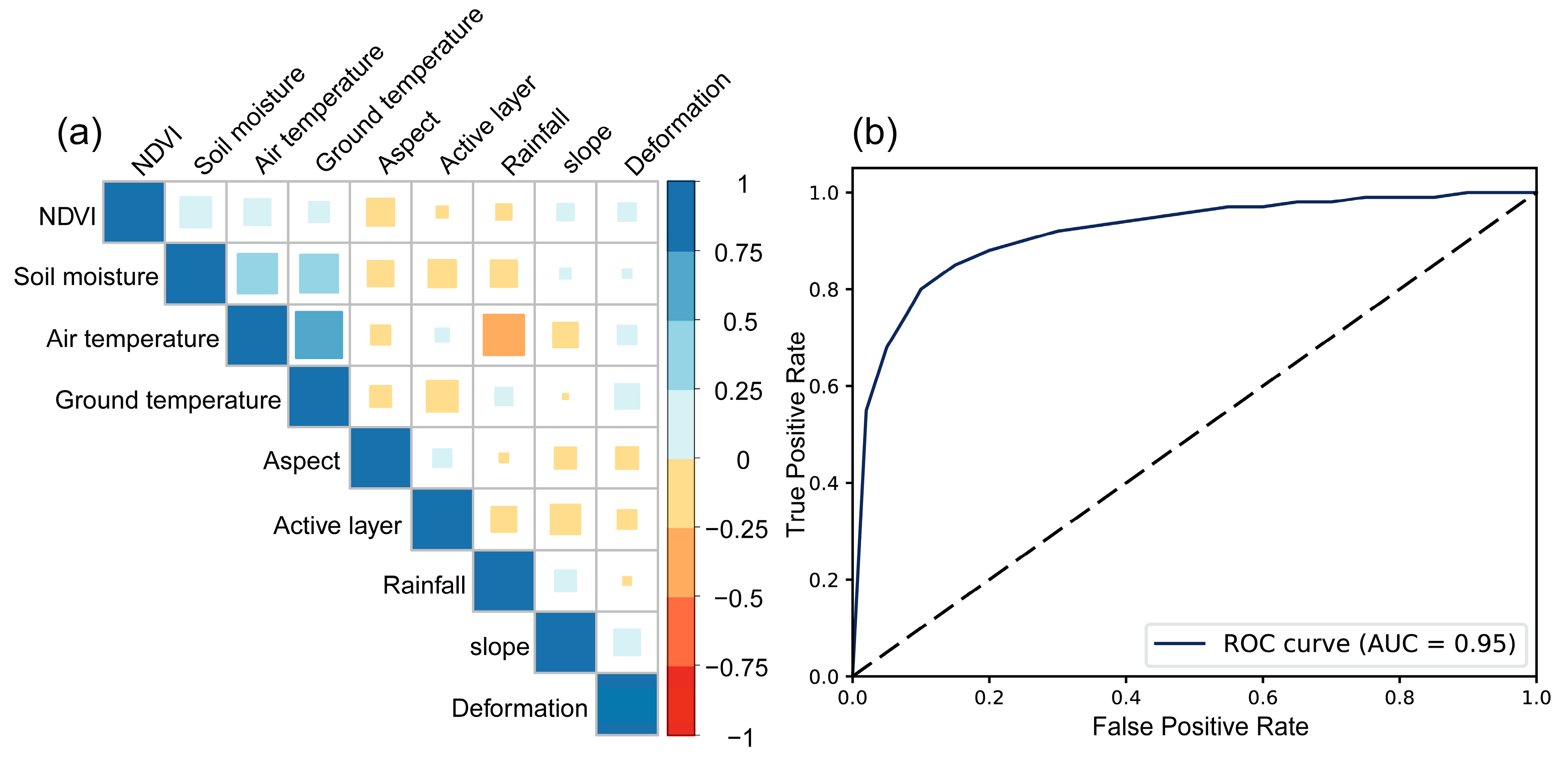
3.3. The Impact of Controlling Factors

The calculated contributions of each disaster-causing factor indicator and the importance coefficients of various factors in thaw slumping are detailed in Figure 9. Temperature is considered the most critical factor affecting the QTEC region. Precipitation is listed as the second most important factor for the development conditions of thaw slumping. Next in importance are slope and surface deformation. Soil moisture, slope aspect, and vegetation coverage are at a moderate level. The active layer and surface temperatures have a minimal impact on thaw slumping. Consequently, it can be seen that thaw slumping in the QTEC region is mainly distributed and induced by climatic factors (temperature and rainfall).

The response curves revealed a nonlinear correlation between the predictor variables and the response factor, suggesting an environment conducive to the occurrence of thaw slumping (Figure 10). The optimal conditions for thaw slumping development in the study area were identified as sudden moderate to high rainfall events (≥18 mm/d). With an increase in temperature, areas of low to medium sensitivity were transformed into highly sensitive areas. Degradation of permafrost in permafrost regions was caused by continuous high temperatures and heavy rainfall, leading to the melting of underground ice, which ultimately resulted in the detachment of the active layer. Such thaw slumping was mainly found distributed on the gentle (0~6°) northern slopes of mountains, where the accumulation of water on gentle slopes led to higher soil moisture content. The development of thaw slumping was also influenced by the type of vegetation, with most thaw slumping in the study area being situated in cold alpine meadows. At surface temperatures of −3.0 to 2.5 °C, the likelihood of thaw slumping occurring was found to be increased. Ground deformation was an important indicator for assessing the stability and degradation of permafrost. When the amount of subsidence exceeded 80 mm, the probability of thaw slumping increased.

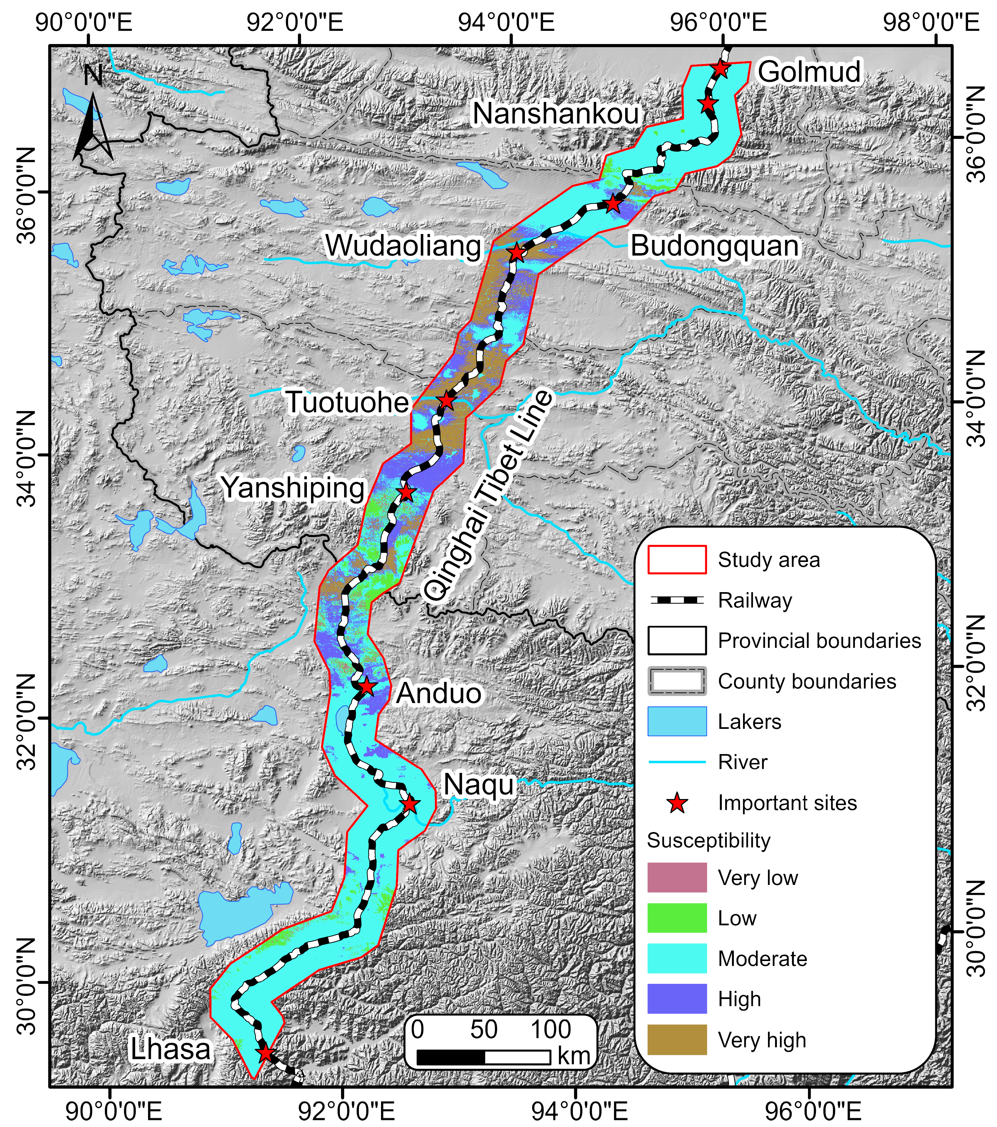
3.4. Thaw Slumping Susceptibility Mapping

The susceptibility of each indicator trained by the radial basis function, combined with GIS spatial analysis, generated the susceptibility of thaw slumping in the study area. The susceptibility values of thaw slumping calculated by the radial basis function were normalized. Then, combined with natural breakpoints, the normalized susceptibility of thaw slumping was reclassified. Based on the principle that higher normalized susceptibility values indicate a higher likelihood of thaw slumping occurrence, the study area was divided into five levels: very low susceptibility zone (0–0.1), low susceptibility zone (0.1–0.3), moderate susceptibility zone (0.3–0.65), high susceptibility zone (0.65–0.9), and very high susceptibility zone (0.9–1), as illustrated in Figure 11.

The areas of the five susceptibility zones were calculated, and detailed area proportion data are presented in

Table 2. Area proportions of each susceptibility zone.

Zone	Area (km2)	Proportion	Thaw Slumping Area (km2)	Proportion
Very low susceptibility	293.11	0.71%	0.04	0.29%
Low susceptibility	2014.2	4.85%	0.44	3.18%
Moderate susceptibility	26,419.85	63.69%	1.90	13.78%
High susceptibility	7700.73	18.56%	3.34	24.26%
Very high susceptibility	5054.11	12.19%	8.04	58.49%

. The high susceptibility zone had an area of 7700.73 km², accounting for 18.56% of the study area. The very high susceptibility zone covered an area of 5054.11 km², representing 12.19% of the study area. The study area was primarily composed of moderate susceptibility zones, with high susceptibility zones mainly distributed in the central region. Upon examining the thaw slumping disaster points, the research indicated that the proportions of the 455 thaw slumping occurrences across susceptibility zones from very low to very high were as follows: 0.29%, 3.18%, 13.78%, 24.26%, and 58.49%, respectively. The distribution of thaw slumping occurrences in susceptibility zones above the high susceptibility zone accounted for a significant 82.75%. This suggested that the susceptibility analysis of thaw slumping along the QTEC in this study was scientifically credible and had achieved the expected zoning effect (Figure 11).

4. Discussion

4.1. Comparison with Existing Studies

Our thaw slump inventory covers the entire QTEC and is relatively comprehensive and up-to-date compared with existing sub-regional thaw slump inventories [44,45]. In 2017, Ref. [45] interpreted 438 RTSs from satellite images, but this only covered the Beiluhe region. When comparing our model with existing models, our U-Net model demonstrated improved accuracy (F1 score = 0.85). Ref. [46] used the DeepLabV3+ model to train on 621 thaw slump features from the Canadian Arctic, with F1 scores ranging from 0.676 to 0.849. Ref. [25] employed a multi-region U-Net3+ model to map RTS features on the Yamal Peninsula, Gydan Peninsula, and six other Arctic regions, with an F1 score of 0.81. However, due to the heterogeneity of thaw slumping features and training data, cross-regional comparison of model performance was challenging. In previous studies [27,29], the sample data used for the susceptibility assessment of thaw slumps in the QTEC were mainly from before 2020. We updated the previous samples with new thaw slumping features, and an accurate and novel sample dataset benefited susceptibility assessment. In total, 455 thaw slumpings were identified across the entire study area, and the susceptibility of thaw slumping in the QTEC was mapped, providing new insights into the impact of climatic and environmental factors on thaw slumps.

4.2. Advantages and Limitations of Thaw Slumping Identification Based on Neural Networks

Collecting historical disaster data is challenging, making it difficult to compile a comprehensive list of thaw slumping incidents in the study area. To address this issue, this study employed deep learning technology, utilizing high-resolution remote sensing imagery data from GaoFen-1 to establish a thaw slumping identification sample library. The identified thaw slumping instances were then used as modeling data for susceptibility assessment.

Deep learning methods provide notable benefits, especially in their capability to automatically acquire features. This contrasts with traditional identification methods that rely on human experience, requiring a substantial amount of data and specialized knowledge. While the model demonstrates high accuracy, there is still a possibility of erroneously identifying other landforms, such as drained ponds and artificial pits. Therefore, it is necessary to filter the identification results through manual review. The deep learning methods used in this study also did not achieve full coverage of thaw slumps, and some thaw slumps re-covered by vegetation could not be identified using only remote sensing images.

4.3. Influencing Factors of Thaw Slump

The assessment of susceptibility to environmental variables in the model holds significant implications. Based on the calculated contributions of various disaster factor indicators, a deeper comprehension can be attained regarding the environmental factors dictating the evolution of thaw slumping within the region. Besides elevation factors taking a dominant role, air temperature and precipitation also play a significant role [47], highlighting the importance of climate in predicting thaw slumping susceptibility. The continuous warming climate and increased instances of sudden rainfall contribute to the heightened absorption of heat by ice-rich slopes [48], consequently resulting in the thawing of permafrost. Although climate remains pivotal, our discoveries also emphasize the substantial influence exerted by local topographical characteristics on the environmental dynamics of thaw slumping [49]. The majority of thaw slumping events are observed on slopes ranging between 2° and 8°. Due to its role as a groundwater collection zone and its possession of a relatively thick layer of fine-grained weathering, the region is more favorable for the formation of substantial subterranean ice deposits.

4.4. Applications of the Susceptibility Map

The susceptibility map of thaw slumping is crucial for formulating sound policies and mitigating the impacts of thaw slumping. The permafrost of the QTP, under the influence of climate change and engineering operations [50], is undergoing a persistent degradation process, which has resulted in the emergence of thaw slumping, and the expedited development of thaw slumps poses significant detrimental effects on regional environments and critical infrastructure. Creating susceptibility maps using neural network models is crucial for the identification and assessment of thaw slumping. This study employed neural network modeling methods using topography, meteorological hydrology, and surface deformation to assess the susceptibility of the QTEC and provided an understanding of the climatic and topographical characteristics of thaw slumping occurrences.

5. Conclusions

This study successfully used deep learning methods to automatically delineate thaw slump areas using high-resolution remote sensing images, providing 455 thaw slump samples for the QTEC and statistically analyzing their spatial distribution characteristics. Concurrently, we proposed a neural network-based modeling method for thaw slumps, employing terrain, climatic, and surface deformation data to map the susceptibility of QTEC to thaw slumps, leading to the following conclusions:

(1) Along the Qinghai–Tibet Engineering Corridor (QTEC), thaw slumps are inclined to develop on north-facing slopes with gentle gradients, and the majority occurred in regions of medium altitude.

(2) The development of thaw slumping is closely related to climatic conditions, especially rainfall and temperature. As long as the terrain and soil conditions are suitable, changes in climate can promote the development of thaw slumping. Under conditions of global warming, some areas of moderate to low susceptibility may transition into high-risk zones.

(3) The study area has 30.75% (approximately 12,754 km²) currently in high to extremely high susceptibility zones, with 82.75% of thaw slump observations situated in areas of high and very high susceptibility. From this perspective, our predictions of present thaw slumping susceptibility are in close agreement with observed outcomes.

References

1. Anisimov, O.A.; Nelson, F.E. Permafrost distribution in the Northern Hemisphere under scenarios of climatic change. Glob. Planet. Chang. 1996, 14, 59–72. [Google Scholar] [CrossRef]
2. Zhou, Y.; Guo, D.; Qiu, G.; Cheng, G.; Li, S. Geocryology in China. Permafr. Periglac. Process. 2000, 12, 315–322. [Google Scholar]
3. Chen, J.; Wu, Y.; O’Connor, M.; Cardenas, M.B.; Schaefer, K.; Michaelides, R.; Kling, G. Active layer freeze-thaw and water storage dynamics in permafrost environments inferred from InSAR. Remote Sens. Environ. 2020, 248, 112007. [Google Scholar] [CrossRef]
4. Liu, S.; Zhao, L.; Wang, L.; Zhou, H.; Zou, D.; Sun, Z.; Xie, C.; Qiao, Y. Intra-Annual Ground Surface Deformation Detected by Site Observation, Simulation and InSAR Monitoring in Permafrost Site of Xidatan, Qinghai-Tibet Plateau. Geophys. Res. Lett. 2022, 49, e2021GL095029. [Google Scholar] [CrossRef]
5. Liu, L.; Schaefer, K.; Zhang, T.; Wahr, J. Estimating 1992–2000 average active layer thickness on the Alaskan North Slope from remotely sensed surface subsidence. J. Geophys. Res. Earth Surf. 2012, 117. [Google Scholar] [CrossRef]
6. Nan, Z.; Li, S.; Cheng, G. Prediction of permafrost distribution on the Qinghai-Tibet Plateau in the next 50 and 100 years. Sci. China Ser. D Earth Sci. 2005, 48, 797–804. [Google Scholar] [CrossRef]
7. Zhao, L.; Wu, Q.; Marchenko, S.S.; Sharkhuu, N. Thermal state of permafrost and active layer in Central Asia during the International Polar Year. Permafr. Periglac. Process. 2010, 21, 198–207. [Google Scholar] [CrossRef]
8. Koven, C.D.; Ringeval, B.; Friedlingstein, P.; Ciais, P.; Cadule, P.; Khvorostyanov, D.; Krinner, G.; Tarnocai, C. Permafrost carbon-climate feedbacks accelerate global warming. Proc. Natl. Acad. Sci. USA 2011, 108, 14769–14774. [Google Scholar] [CrossRef] [PubMed]
9. Zhang, Z.; Wang, M.; Wu, Z.; Liu, X. Permafrost deformation monitoring along the Qinghai-Tibet Plateau engineering corridor using InSAR observations with multi-sensor SAR datasets from 1997–2018. Sensors 2019, 19, 5306. [Google Scholar] [CrossRef]
10. Howard, H.R.; Manandhar, S.; Wang, Q.; Mcmillan, J.M.; Qie, G.; Liu, X.; Thapa, K.; Xu, X.; Wang, G. Spatially characterizing land surface deformation and permafrost active layer thickness for Donnelly installation of Alaska using DInSAR and MODIS data. Cold Reg. Sci. Technol. 2022, 196, 103510. [Google Scholar] [CrossRef]
11. Aas, K.S.; Martin, L.; Nitzbon, J.; Langer, M.; Boike, J.; Lee, H.; Berntsen, T.K.; Westermann, S. Thaw processes in ice-rich permafrost landscapes represented with laterally coupled tiles in a land surface model. Cryosphere 2019, 13, 591–609. [Google Scholar] [CrossRef]
12. Zhang, M.; Wang, B.; Wang, D.; Ye, W.; Guo, Z.; Gao, Q.; Yue, G. The effects of rainfall on the surface radiation of permafrost regions in Qinghai-Tibet Plateau: A case study in Beiluhe area. J. Glaciol. Geocryol 2021, 43, 1092–1101. [Google Scholar]
13. Zhang, X.; Zhang, H.; Wang, C.; Tang, Y.; Zhang, B.; Wu, F.; Wang, J.; Zhang, Z. Time-series InSAR monitoring of permafrost freeze-thaw seasonal displacement over Qinghai–Tibetan Plateau using Sentinel-1 data. Remote Sens. 2019, 11, 1000. [Google Scholar] [CrossRef]
14. Grosse, G.; Harden, J.; Turetsky, M.; McGuire, A.D.; Camill, P.; Tarnocai, C.; Frolking, S.; Schuur, E.A.G.; Jorgenson, T.; Marchenko, S.; et al. Vulnerability of high-latitude soil organic carbon in North America to disturbance. J. Geophys. Res. Biogeosciences 2011, 116. [Google Scholar] [CrossRef]
15. Lantuit, H.; Pollard, W.H.; Couture, N.; Fritz, M.; Schirrmeister, L.; Meyer, H.; Hubberten, H.W. Modern and late Holocene retrogressive thaw slump activity on the Yukon coastal plain and Herschel Island, Yukon Territory, Canada. Permafr. Periglac. Process. 2012, 23, 39–51. [Google Scholar] [CrossRef]
16. Li, Y.; Jin, H.; Wen, Z.; Wen, Z.; Zhao, Z.; Jin, X. Stability of permafrost slopes: A review. J. Glaciol. Geocryol. 2022, 44, 203–216. [Google Scholar]
17. Ni, J.; Wu, T.; Zhu, X.; Hu, G.; Zou, D.; Wu, X.; Li, R.; Xie, C.; Qiao, Y.; Pang, Q.; et al. Simulation of the present and future projection of permafrost on the Qinghai-Tibet Plateau with statistical and machine learning models. J. Geophys. Res. Atmos. 2021, 126, e2020JD033402. [Google Scholar] [CrossRef]
18. Ramage, J.L.; Irrgang, A.M.; Herzschuh, U.; Morgenstern, A.; Couture, N.; Lantuit, H. Terrain controls on the occurrence of coastal retrogressive thaw slumps along the Yukon Coast, Canada. J. Geophys. Res. Earth Surf. 2017, 122, 1619–1634. [Google Scholar] [CrossRef]
19. Lantuit, H.; Pollard, W.H. Fifty years of coastal erosion and retrogressive thaw slump activity on Herschel Island, southern Beaufort Sea, Yukon Territory, Canada. Geomorphology 2008, 95, 84–102. [Google Scholar] [CrossRef]
20. Jones, M.K.W.; Pollard, W.H.; Jones, B.M. Rapid initialization of retrogressive thaw slumps in the Canadian high Arctic and their response to climate and terrain factors. Environ. Res. Lett. 2019, 14, 055006. [Google Scholar] [CrossRef]
21. Linlin, L.; Liming, J.; Zhiwei, Z.; Yuxing, C.; Yafei, S. Object-oriented classification of unmanned aerial vehicle image for thermal erosion gully boundary extraction. Remote Sens. Land Resour. 2019, 31, 180–186. [Google Scholar]
22. Witharana, C.; Udawalpola, M.R.; Liljedahl, A.K.; Jones, M.K.W.; Jones, B.M.; Hasan, A.; Joshi, D.; Manos, E. Automated detection of retrogressive thaw slumps in the high Arctic using high-resolution satellite imagery. Remote Sens. 2022, 14, 4132. [Google Scholar] [CrossRef]
23. Abolt, C.J.; Young, M.H. High-resolution mapping of spatial heterogeneity in ice wedge polygon geomorphology near Prudhoe Bay, Alaska. Sci. Data 2020, 7, 87. [Google Scholar] [CrossRef] [PubMed]
24. Nitze, I.; Heidler, K.; Barth, S.; Grosse, G. Developing and testing a deep learning approach for mapping retrogressive thaw slumps. Remote Sens. 2021, 13, 4294. [Google Scholar] [CrossRef]
25. Yang, Y.; Rogers, B.M.; Fiske, G.; Watts, J.; Potter, S.; Windholz, T.; Mullen, A.; Nitze, I.; Natali, S.M. Mapping retrogressive thaw slumps using deep neural networks. Remote Sens. Environ. 2023, 288, 113495. [Google Scholar] [CrossRef]
26. Kaur, H.; Gupta, S.; Parkash, S.; Thapa, R. Knowledge-driven method: A tool for landslide susceptibility zonation (LSZ). Geol. Ecol. Landsc. 2023, 7, 1–15. [Google Scholar] [CrossRef]
27. Yin, G.; Luo, J.; Niu, F.; Liu, M.; Gao, Z.; Dong, T.; Ni, W. High-resolution assessment of retrogressive thaw slump susceptibility in the Qinghai-Tibet Engineering Corridor. Res. Cold Arid. Reg. 2023, 15, 288–294. [Google Scholar] [CrossRef]
28. Rudy, A.C.; Lamoureux, S.F.; Treitz, P.; Van Ewijk, K.Y. Transferability of regional permafrost disturbance susceptibility modelling using generalized linear and generalized additive models. Geomorphology 2016, 264, 95–108. [Google Scholar] [CrossRef]
29. Yin, G.; Luo, J.; Niu, F.; Lin, Z.; Liu, M. Machine learning-based thermokarst landslide susceptibility modeling across the permafrost region on the Qinghai-Tibet Plateau. Landslides 2021, 18, 2639–2649. [Google Scholar] [CrossRef]
30. Jiang, Y.; Yang, K.; Qi, Y.; Zhou, X.; He, J.; Lu, H.; Li, X.; Chen, Y.; Li, X.; Zhou, B.; et al. TPHiPr: A long-term (1979–2020) high-accuracy precipitation dataset (1/30°, daily) for the Third Pole region based on high-resolution atmospheric modeling and dense observations. Earth Syst. Sci. Data 2023, 15, 621–638. [Google Scholar] [CrossRef]
31. Niu, F.; Yin, G.; Luo, J.; Lin, Z.; Liu, M. Permafrost distribution along the Qinghai-Tibet Engineering Corridor, China using high-resolution statistical mapping and modeling integrated with remote sensing and GIS. Remote Sens. 2018, 10, 215. [Google Scholar] [CrossRef]
32. Marmanis, D.; Datcu, M.; Esch, T.; Stilla, U. Deep learning earth observation classification using ImageNet pretrained networks. IEEE Geosci. Remote Sens. Lett. 2015, 13, 105–109. [Google Scholar] [CrossRef]
33. Eigen, D.; Fergus, R. Predicting depth, surface normals and semantic labels with a common multi-scale convolutional architecture. In Proceedings of the IEEE International Conference on Computer Vision, Santiago, Chile, 7–13 December 2015; pp. 2650–2658. [Google Scholar]
34. Sun, C.; Zhao, H.; Mu, L.; Xu, F.; Lu, L. Image semantic segmentation for autonomous driving based on improved U-Net. Cmes-Comput. Model. Eng. Sci. 2023, 136, 787–801. [Google Scholar] [CrossRef]
35. Yu, B.; Lane, I. Multi-task deep learning for image understanding. In Proceedings of the 2014 6th International Conference of Soft Computing and Pattern Recognition (SoCPaR), Tunis, Tunisia, 11–14 August 2014; pp. 37–42. [Google Scholar]
36. Li, X.; Liu, Z.; Luo, P.; Change Loy, C.; Tang, X. Not all pixels are equal: Difficulty-aware semantic segmentation via deep layer cascade. In Proceedings of the IEEE Conference on Computer Vision and Pattern Recognition, Honolulu, HI, USA, 21–26 July 2017; pp. 3193–3202. [Google Scholar]
37. Jiang, X.; Jiang, J.; Yu, J.; Wang, J.; Wang, B. MSK-UNET: A Modified U-Net Architecture Based on Selective Kernel with Multi-Scale Input for Pavement Crack Detection. J. Circuits Syst. Comput. 2023, 32, 2350006. [Google Scholar] [CrossRef]
38. Alexandridis, A.; Chondrodima, E.; Sarimveis, H. Radial basis function network training using a nonsymmetric partition of the input space and particle swarm optimization. IEEE Trans. Neural Netw. Learn. Syst. 2012, 24, 219–230. [Google Scholar] [CrossRef] [PubMed]
39. Zhang, P.; Zhou, X.; Pelliccione, P.; Leung, H. RBF-MLMR: A multi-label metamorphic relation prediction approach using RBF neural network. IEEE Access 2017, 5, 21791–21805. [Google Scholar] [CrossRef]
40. Liu, K.; Zhang, R.; Cui, Z.B.; Zhang, D.; Gao, S. Research on cloud model optimization radial basis function neural network algorithm. J. Henan Univ. Sci. Technol. (Nat. Sci.) 2023, 44, 49–55. [Google Scholar]
41. Chen, S. Orthogonal Least Sequares Learning Algorithm for Radial Basis Function Networks. IEEE Trans. Neural Netw. 1991, 4, 246–257. [Google Scholar]
42. Sun, Z.; Zhang, S. A radial basis function approximation method for conservative Allen–Cahn equations on surfaces. Appl. Math. Lett. 2023, 143, 108634. [Google Scholar] [CrossRef]
43. Liu, M.; Peng, W.; Hou, M.; Tian, Z. Radial basis function neural network with extreme learning machine algorithm for solving ordinary differential equations. Soft Comput. 2023, 27, 3955–3964. [Google Scholar] [CrossRef]
44. Niu, F.; Luo, J.; Lin, Z.; Fang, J.; Liu, M. Thaw-induced slope failures and stability analyses in permafrost regions of the Qinghai-Tibet Plateau, China. Landslides 2016, 13, 55–65. [Google Scholar] [CrossRef]
45. Luo, J.; Niu, F.; Lin, Z.; Liu, M.; Yin, G. Recent acceleration of thaw slumping in permafrost terrain of Qinghai-Tibet Plateau: An example from the Beiluhe Region. Geomorphology 2019, 341, 79–85. [Google Scholar] [CrossRef]
46. Huang, L.; Lantz, T.C.; Fraser, R.H.; Tiampo, K.F.; Willis, M.J.; Schaefer, K. Accuracy, efficiency, and transferability of a deep learning model for mapping retrogressive thaw slumps across the Canadian Arctic. Remote Sens. 2022, 14, 2747. [Google Scholar] [CrossRef]
47. Karjalainen, O.; Luoto, M.; Aalto, J.; Hjort, J. New insights into the environmental factors controlling the ground thermal regime across the Northern Hemisphere: A comparison between permafrost and non-permafrost areas. Cryosphere 2019, 13, 693–707. [Google Scholar] [CrossRef]
48. Xia, Z.; Huang, L.; Fan, C.; Jia, S.; Lin, Z.; Liu, L.; Luo, J.; Niu, F.; Zhang, T. Retrogressive thaw slumps along the Qinghai-Tibet Engineering Corridor: A comprehensive inventory and their distribution characteristics. Earth Syst. Sci. Data Discuss. 2022, 14, 3875–3887. [Google Scholar] [CrossRef]
49. Karjalainen, O.; Luoto, M.; Aalto, J.; Etzelmüller, B.; Grosse, G.; Jones, B.M.; Lilleøren, K.S.; Hjort, J. High potential for loss of permafrost landforms in a changing climate. Environ. Res. Lett. 2020, 15, 104065. [Google Scholar] [CrossRef]
50. Wang, R.; Guo, L.; Yang, Y.; Zheng, H.; Liu, L.; Jia, H.; Diao, B.; Liu, J. Thermokarst Lake Susceptibility Assessment Induced by Permafrost Degradation in the Qinghai–Tibet Plateau Using Machine Learning Methods. Remote Sens. 2023, 15, 3331. [Google Scholar] [CrossRef]
Figure 1. Map of the study area.
Sustainability 16 05120 g001
Figure 2. Flowchart of the methodology.
Sustainability 16 05120 g002
Figure 3. U-Net network architecture diagram.
Sustainability 16 05120 g003
Figure 4. Construction of susceptibility indices for thaw slumping in the study area and disaster-causing data: (a) aspect data; (b) slope data; (c) NDVI data; (d) ground temperature data; (e) rainfall data; (f) soil moisture data; (g) air temperature data daily; (h) SBAS-InSAR time-series surface deformation data; (i) active layer thickness data.
Sustainability 16 05120 g004
Figure 5. (a) Distribution of thaw slumps identified within the study area. (b) A UAV image of thaw slump near the Qinghai–Tibet railway (center location: 92.936° E, 34.855° N). (c) Field survey photograph (by Pengfei Li).
Sustainability 16 05120 g005
Figure 6. Models for determining the contour of the same thaw slump: (a) ResNet101, (c) ResNet152, and (e) VGG16. The loss functions of the three neural networks during training and validation processes: (b) ResNet101, (d) ResNet152, and (f) VGG16.
Sustainability 16 05120 g006
Figure 7. Frequency distribution of thaw slumping along the Qinghai–Tibet Engineering Corridor (QTEC). (a) Histogram showing the perimeter sizes of all thaw slumping. (b) Histogram showing the areas of all thaw slumping. (c) Elevation frequency of all thaw slumping. (d) Slope frequencies of all thaw slumping. (e) Deformation frequency of all thaw slumping. (f) Frequency distribution of all thaw slumping in each slope orientation class.
Sustainability 16 05120 g007
Figure 8. (a) Pearson’s correlations between factors for thaw slumping. (b) ROC curve of thaw slumping susceptibility prediction model.
Sustainability 16 05120 g008
Figure 9. The normalization importance of factors for thaw slumping.
Sustainability 16 05120 g009
Figure 10. Response curves for the disaster-causing factors.
Sustainability 16 05120 g010
Figure 11. Susceptibility zoning of thaw slumping along the Qinghai–Tibet Engineering Corridor (QTEC).
Sustainability 16 05120 g011