Abstract
The Pesaro-Urbino province (PUP) (northern Marche, central Italy) is one of the most seismically active areas in Italy, with the most recent earthquakes (5.2 and 5.5 Mw) having occurred on 9 November 2022 with an epicenter located in the Adriatic Sea. A detailed geochemical and isotopic characterization of 87 groundwaters (and dissolved gases) circulating in the PUP was carried out to (i) unravel the geochemical processes controlling the water circulation, (ii) investigate the interplay between deep originated fluids and shallow aquifers, (iii) evaluate the reliability of specific geochemical parameters as tracers for seismic activity, and (iv) select the most suitable sampling sites to deploy a monitoring network to highlight possible compositional changes related to the regional and local tectonic activity. The geochemical dataset includes waters showing five different hydrochemical compositional facies: (i) calcium bicarbonate with low Total Dissolved Solids (TDS); (ii) calcium bicarbonate with relatively high concentrations of sulfate (>200 mg/L); (iii) sodium bicarbonate with pH > 8.8; (iv) calcium sulfate; (v) sodium chlorine. Two distinct groups of dissolved gases can be recognized: (a) N2-dominated gases with N2/Ar ratios similar to those of Air-Saturated Water (ASW); (b) CO2- and CH4-rich gases associated with high TDS and springs rich in S-bearing reduced species. The isotopic values of δ13C-CO2 and δ13C-CH4 suggest a predominant biogenic origin for both species with a negligible contribution from deep-seated fluids. The Ca-HCO3(SO4), Ca(Na)-SO4(Cl), and Na-HCO3 waters, being likely related to deep hydrological pathways, are the best candidates to be included in the monitoring network in the Pesaro-Urbino province. This will be of paramount importance in addressing the challenge of unravelling fluid geochemical precursors of earthquakes, thus increasing and improving seismic surveillance practices and hazard mitigation.
1. Introduction
Among natural phenomena, earthquakes represent the deadliest catastrophic events, considering the yearly occurrences of seismic events and the high number of fatalities, injuries, and damages to the infrastructures and the respective high economic impact [1]. Italy is one of the most seismically active countries in the world, being located between the African and Euro-Asiatic plates and characterized by an anticlockwise rotation, which is still ongoing today [2]. Along the Italian peninsula, many areas are indeed affected by intense and continuous seismic activity, e.g., the Sibillini and Gran Sasso areas in the Central Apennines [3,4,5,6], while others are less frequently active but capable of experiencing high-magnitude earthquakes (up to 7 Mw; [5]). Among the latter, the province of Pesaro-Urbino (hereafter, PU) (northern Marche, central Italy) is marked by two primary composite seismogenic source areas that may generate earthquakes with a magnitude of up to >6.5 Mw [5]. The first one is located in the Umbria–Marche Apennines, while the second one occurs along the Adriatic coast extending between Cattolica and Ancona cities (Figure 1). The PU province experienced high seismicity in the past, e.g., the 1781 Cagli earthquake (6.4 Mw), which caused approximately 300 deaths [6], and the 1930 Senigallia earthquake (5.8 Mw), during which 18 people lost their lives [7]. The last events (5.2 and 5.5 Mw) occurred on 9 November 2022. A rapid sequence of seismic shocks, a few minutes from each other, with the epicenter located in the Adriatic Sea, 35 km away from the city of Pesaro, affected the majority of the Marche Region. Fortunately, no casualties or significant damages were recorded.
Even though the prediction of earthquakes is challenging, promising geochemical precursors were recently recognized in different geological and geodynamic contexts worldwide, through long-term (periodical or continuous) monitoring of various chemical, physical, isotopic, or hydrogeological parameters, e.g., [8,9,10,11,12,13,14,15,16,17,18,19,20,21,22,23,24,25]. Precursors (or tracers) of seismic events can be defined as a “quantitatively measurable change in an environmental parameter occurring prior to the mainshock” [26,27,28,29,30]. These changes may occur from months to weeks prior to the event or concurrently and are generally observed for earthquakes having a magnitude higher than 4 Mw [9,14,30].
Precursory changes observed in geofluids are considered tracers of the evolution of the stress field over time, and, hence, related to the faulting activity occurring during seismogenesis [29,31]. In fact, an increase in stress or strain rate, micro-fracturing, and faulting can trigger several physical mechanisms and chemical processes able to produce significant changes that can be recorded at the surface [14,30]. A detailed and continuous geochemical characterization of the circulating groundwaters is of pivotal importance to highlight possible modifications in terms of water chemistry and isotopes. Reliable precursory signals of seismic activity can, thus, be recorded, being, in most cases, extremely site-specific and strictly connected to the geological, hydrogeological, and tectonic characteristics of a given area [25,26,27,30].
Changes in geochemical parameters of groundwaters before seismic events have repeatedly been observed. For example, water springs and groundwaters modified their original composition (i.e., increased their trace element contents) prior to the 2016 Amatrice-Norcia seismic sequence in central Italy [19], while variations in the water isotopic composition (i.e., δ18O-H2O) were observed before and after the 2016 Kumamoto earthquake (7.0 Mw) in Japan [21,22]. Moreover, changes in the discharge rate of streams and springs were frequently reported, e.g., after the 2007 Alum Rock earthquake (5.6 Mw) [32] and the 2014 South Napa earthquake (6.0 Mw) [33], both occurring in California. A significant increase in the emission rate of dissolved Rn was detected prior to the 1995 Kobe earthquake (6.9 Mw) [34] and before the 2013 Rueisuei earthquake (6.4 Mw, eastern Taiwan; [35]). Also relatively common is the variation in the piezometric level of shallow-to-deep wells, related to events of strong magnitudes, e.g., the 2004 Sumatra-Andaman earthquake (9.0 Mw). Interestingly, changes in the water level were recorded even thousands of kms away from the epicenter [20,36,37].
In the present study, a large-scale sampling survey was carried out during the spring and autumn of 2022 by collecting 145 water samples (83 in May and 62 in November) from different types of emergences (i.e., springs, wells, and ditches) and in various geological–structural settings of the Umbria–Marche Apennines.
Considering that, to the best of our knowledge, the geochemical features of the fluids circulating in the PU province have poorly been investigated, e.g., [38,39,40,41], the main goal of such a detailed sampling campaign was to provide in-depth information about the geochemical and isotopic composition of the waters (and dissolved gases) discharging in the study area, in order to (i) describe the main geochemical processes occurring along the hydrological pathways that control the chemistry of springs and wells, in relation to the geological and hydrogeological framework (e.g., limestones, clays, and alluvial deposits), as well as the climatic conditions and (ii) explore the relationship between shallow aquifers and deep-circulating fluids. Our results are aimed at identifying the most suitable sampling sites for monitoring the most reliable geochemical signals related to an impending seismic event, a paramount step to increasing seismic surveillance measures and sustainability.
2. Geological and Seismo-Tectonic Background
The PU province is located in the northern Marche Region (central Italy) within the Umbria–Marche Apennines, which represent the external part of the Northern Apennines developed during the Miocene.
The area is characterized by a strongly variable topography, which ranges from a maximum altitude of 1.701 m (Mt. Catria) to sea level, and a complex geological setting (Figure 1). The outcropping geological formations that outcrop in the study area span from the Lower Jurassic, in the north-western portion, to the Miocene–Pleistocene deposits occurring in the Adriatic coastal area eastward, partially covered by the recent Quaternary alluvial deposits [42,43,44,45,46,47,48,49,50,51].

Figure 1.
Geological map of the Pesaro-Urbino province [51] and location of the sampling points. Major seismogenetic structures are reported after [5]. See the text for more information on the different lithologies of the geological formations. Black dashed lines represent the borders of the sampling areas: NC (Nerone–Catria Ridge), FU (Furlo Gorge), CS (Cesane Ridge), BS (Bellisio Solfare), IZ (Internal Zone), CZ (Coastal Zone), and NB (Northern Border).

The Umbria–Marche Apennines are defined as an arcuate fold-and-thrust belt, verging towards E-NE, with a major detachment in the Triassic Evaporitic Burano Formation and displaced by several thrust fold systems (NNW-SSE) and strike-slip faults with N-S and E-W orientation [49]. It also comprises the boundary between the Tyrrhenian Umbro–Tuscan extensional area and the Adriatic compressional zone [52].
The study area has recently experienced moderate seismicity, in terms of both magnitudes and frequency of events, related to the presence of two major composite seismogenic sources [5] located in (a) the Umbria–Marche Apennines, along the Mt. Catria–Mt. Nerone Ridge, and (b) on the Adriatic coast and off-shore areas (Figure 1). The strongest and most destructive events that occurred within the Apennine chain are generally associated with distensive focal mechanisms [53,54,55,56]. On the other hand, the Cagli area and its surroundings (Figure 1) are characterized by the occurrence of NW–SE-oriented compressive structures (e.g., the 1781 Cagli earthquake, Mw = 6.4) that developed during the Upper Miocene–Pliocene tectonic phases [2]. However, recent studies highlighted the presence of a recently activated normal fault system, probably related to Quaternary faulting in the Mt. Nerone area, which was possibly the source of the 1781 earthquake [57]. Seismic activity on the Adriatic coast (and off-shore), associated with compressive and transpressive structures, is less frequent and shows lower-magnitude events (i.e., generally Mw < 6; [58,59,60,61,62,63]).
The Umbria–Marche Apennines show a thick and extremely articulated sedimentary succession that started with the deposition of carbonate platform limestones, i.e., Calcare Massiccio Fm (Lower Jurassic). Although not outcropping in the study area, the Burano Fm widespread area occurs at the bottom of the Umbria–Marche succession [40,51,64] and was drilled at 620 and 1550 m depth in the Burano 001 and Fossombrone 001 wells in the Burano River gorge and Cesane Ridge areas, respectively [65,66,67].
The subsequent break-up of the carbonatic platform led to the development of intra-basinal highs and lows with ongoing carbonate sedimentation characterized by micritic pelagic limestones with cherty nodules (Corniola Fm), marly limestones, and marls (Rosso Ammonitico and Marne a Posidonia Fm), and then micritic limestones with cherts and calcarenites (Calcari Diasprini Fm). The complete Jurassic succession deposited on structural lows is found in Mt. Nerone and Mt. Catria, whereas the condensed succession (Bugarone Fm) was deposited on structural highs [42,44,51,68,69]. The transition from the Maiolica Fm (mainly limestone and dolomitic limestones) to the Marne a Fucoidi Fm (an alternating marly-to-clay succession) marked the end of the predominant carbonate sedimentation and the beginning of a uniform marly sedimentation [47,70] that continued throughout the Cretaceous to Eocene with the deposition of the Scaglia Fms, i.e., Scaglia Bianca, Scaglia Rossa, Scaglia Variegata, and Scaglia Cinerea. Eventually, the Bisciaro Fm (marly limestones, marls, and clays with volcanoclastic levels) and the Schlier Fm (marls and clays with locally marly limestones and calcarenites) preceded the turbiditic sedimentation that started from the Early Miocene following the shortening of the Umbria–Marche domain [51]. In this portion of the Northern Apennines, the siliciclastic succession is almost exclusively represented by the Marnoso Arenacea Fm (Marchigiana vs. Umbro–Romagnola, Figure 1) that extends for hundreds of km from the Emilia Romagna to the Umbria–Marche Apennines and consists of turbiditic sandstones and siltstones interlayered with marlstones [46,71,72]. The Marnoso Arenacea Fm is overlain by the Tripoli Fm (bituminous clays, marls, sandstones, and diatomites) belonging to the Messinian Evaporite succession [51,73]. The coastal area of the PU Province is mainly composed of silty clays interbedded with sandstones, clays, and evaporites, deposited starting from the Late Miocene to Pleistocene (i.e., Tripoli, Gessoso-Solfifera, San Donato, Colombacci, and Argille Azzurre Fms) and overlain by the Quaternary alluvial–marine deposits associated with the Foglia and Metauro river valleys [74,75,76].
3. Materials and Methods
For this study, 145 samples from the PU province were collected from 64 springs, 19 wells, and 3 ditches (SM1), selected based on their spatial location to cover as much as possible the studied area. One additional sample was collected from the Cesano River. The sampling survey was carried out twice to highlight and evaluate possible seasonal changes. The first campaign was carried out in May–June 2022 (83 samples) while the second one was in November 2022 (62 samples). It is worth mentioning that not all the samples were collected in the second fieldwork due to the severe damages caused by the disastrous flood that hit the PU and Ancona provinces between 15 and 16 September 2022 [77], making a few sampling points either not accessible or disappeared.
The study area was subdivided into seven groups, based on their geographic–geological features (Figure 1): (1) NC 1-31 (Nerone–Catria Ridge), (2) BS 1-5 (Bellisio Solfare), (3) FU 1-12 (Furlo Gorge), (4) CS 1-6 (Cesane Ridge), (5) IZ 1-18 (Internal Zone), (6) NB 1-10 (Northern Border) and (7) CZ 1-5 (Coastal Zone). From January 2023 to January 2024, rainwater samples were collected from four sites located at different altitudes in the study area (Fano 14 m asl; Urbino 476 m asl; Serravalle di Carda 783 m asl; Mt. Nerone 1267 m asl), using Palmex Ltd. rain samplers [78].
Water temperature (T, in °C), pH, electrical conductivity (EC, in μS/cm at 25 °C), and redox potential (Eh, in meV), were measured in situ using an XS PC70+ DHS multiparametric probe. Different water aliquots were collected at each sampling point, as follows: (i) unfiltered aliquot in 125 mL polyethylene (PE) bottle for the analysis of anions (Cl−, SO42−, NO3−, Br−, F−), NH4+, SiO2, B, and HCO3−; (ii) filtered (0.45 μm) and acidified (with 1% Suprapur HCl) aliquot in 50 mL PE bottle for the analysis of major cations (Ca2+, Mg2+, Na+, K+); (iii) filtered (0.45 μm) and acidified (with 1% Suprapur HNO3) aliquot in 50 mL PE bottle for trace elements (Li, Al, V, Cr, Mn, Fe, Co, Ni, Cu, Zn, As, Se, Rb, Sr, Cs, Ba, Pb); (iv) filtered aliquot in 15 mL plastic tube for the analysis of water isotopes. An additional unfiltered aliquot in 40 mL glass vials equipped with a pierceable cap for the analysis of major dissolved gases (CO2, CH4, N2, Ar, O2, and He) was also collected in 27 and 18 selected samples in spring and autumn 2022, respectively. The selection of these samples was based on their geochemical features and geographic location. In February 2023, another unfiltered aliquot in pre-evacuated 250 mL glass flasks equipped with Thorion® valves was collected from 17 sampling points for the analysis of δ13C-CO2 and δ13C-CH4 in the dissolved gas phase.
Total alkalinity was analyzed within 24–48 h from the sampling by acidimetric titration (AT) using an automatic burette filled with 0.01 M HCl and methyl orange as the colorimetric indicator. Major cations and anions were analyzed by ion chromatography (IC), using Metrohm 861 Compact IC and Metrohm 761 Advanced Compact IC chromatographs, respectively. Ammonia (NH4+) was analyzed by molecular spectrophotometry (MSP) using a HACH DR2010 instrument. The analytical errors for AT, IC, and MSP were <5% [79]. Data quality for major components was evaluated using the electroneutrality parameter, which was always in the range of ±5%. Trace elements were measured by Inductively Coupled Plasma Mass Spectrometry (ICP-MS) using an Agilent 7800 Mass Spectrometer with an analytical error below 10%. The accuracy and precision of the analysis were tested using internal and international standards, i.e., Aqua 1 e Srls 6 (CNRS-Canada) and DW1 (ISC Science). The isotopic analyses of the oxygen (18O/16O and expressed as δ18O ‰ vs. V-SMOW) and hydrogen (2H/1H and expressed as δ2H ‰ vs. V-SMOW) were performed using a near-infrared laser analyzer (Picarro L2130-i) using wavelength-scanned cavity ring-down spectroscopy technique (WS-CRDS, analytical errors: δ18O ± 0.08‰ and δ2H ± 0.5‰ vs. V-SMOW) [79].
The concentrations of dissolved gases were analyzed by gas chromatography (GC) using different instruments: (i) CO2, N2, (Ar + O2), and He using a Shimadzu 15A instrument equipped with a 5 m long stainless-steel column with Porapak 80/100 mesh and a TCD; (ii) Ar and O2 using a Thermo Focus gas chromatograph equipped with a 30 m long capillary molecular sieve column and a TCD; (iii) CH4 using a Shimadzu 14A gas chromatograph equipped with an FID and a 10 m long stainless-steel column packed with Chromosorb PAW 80/100 mesh coated with 23% SP 1700 [80]. The total concentrations of dissolved gases (in mmol/L) were obtained by the sum of ni;g, i.e., the moles of the i gas in the sampling flasks’ headspace measured by gas chromatography, and ni;l, i.e., the moles of the i gas that remained in the water collected in the sampling flasks. The ni;l values were recalculated from the ni;g, by means of the Henry’s law constants at standard conditions [81], assuming that the separated gas phase was in equilibrium with the liquid phase. The analytical error for GS was below 5% [80]. The isotopic analysis of carbon (13C/12C) in both carbon dioxide (CO2) and methane (CH4), expressed as δ13C-CO2 and δ13C-CH4 ‰ vs. V-PDB, respectively, was measured through WS-CRDS using a Picarro G2201-i. The analytical errors for WS-CRDS were ±0.16‰ and ±1.15‰ vs. V-PDB for δ13C-CO2 and δ13C-CH4, respectively [82]. All chemical and isotopic analyses of waters and dissolved gases were carried out at the Laboratory of Fluid Geochemistry at the Department of Earth Sciences (University of Florence, Italy), except those of SiO2 (expressed as SiO2; method APAT CNR IRSA 4130 Man 29 2003) and B (method EPA 6020B, 2014), which were performed at the laboratories of Gruppo C.S.A. S.p.A (Rimini, Italy).
4. Results
4.1. Water Chemical and Isotopic Composition
The complete results of both the spring 2022 and autumn 2022 sampling campaigns (including the physicochemical parameters, major and trace elements, and water-stable isotopes) are reported in the Supplementary Materials (S1). Water sample IDs refer to their geographic provenance: NC (Nerone–Catria Ridge), BS (Bellisio Solfare), FU (Furlo Gorge), CS (Cesane Ridge), IZ (Internal Zone), NB (Northern Border), and CZ (Coastal Zone) as reported in Figure 1.
The pH spanned from 6.92 to 9.45 in spring and from 6.61 to 9.40 in autumn, with most samples showing from neutral to slightly alkaline values. A few springs, commonly called “sulfur springs”, being characterized by the typical odor of rotten eggs and the occurrence of colloidal sulfur, e.g., [83,84], showed an alkaline pH generally higher than 8.8. Water temperature ranged between 9.0 and 20.7 °C (spring 2022) and from 7.3 to 17.3 °C (autumn 2022). The Eh values ranged from −245 to 238 meV and from −280 to 202 meV, in spring and autumn, respectively. Negative Eh values were measured for the sulfur springs and some high Total Dissolved Solids (hereafter, TDS) springs (i.e., NC-27, NC-28, NC-30, BS-01, IZ-13, IZ-14, IZ-15, IZ-16); additionally, in autumn, the sample (BS-05) collected from the river nearby a mineral spring (BS-01) showed a value of −80 meV.
The TDS showed a large variability in both sampling surveys, being comprised from 230 to 4930 mg/L (spring), and 270 to 3930 mg/L (autumn). As far as major anions are concerned (Figure 2A), HCO3− was the main component in those samples, characterized by low-to-medium TDS values (<1200 mg/L). Sulfur springs, showing pH values > 8.8, had CO32− concentrations ranging from 5 to 43 mg/L in spring, and from 14 to 38 mg/L in autumn. The higher the TDS values, the higher the Cl− (up to 1280 mg/L) and SO42− (up to 1950 mg/L). Chloride was the main component in ditches and in the IZ-16 sample, while the sulfate was dominant in those samples collected from high TDS springs. Nitrate contents were generally low in most samples, although a general increase from west to east was observed, with the higher values being detected for the CZ waters, e.g., CZ-01 (77 mg/L in spring, and 96 mg/L in autumn), CZ-02 (92 mg/L in spring, and 85 mg/L in autumn), and CZ-03 (64 in spring, and 68 mg/L in autumn), which circulate near the Metauro Plain, where nitrate contamination has been documented by e.g., [85,86]. The peak value for NO3− was measured in the IZ-10 sample (autumn, 130 mg/L). Among minor anions, F− and Br− were generally ≤1 mg/L, with the latter being below the detection limit (0.01 mg/L) for a few samples. Nevertheless, both species showed the highest contents in high TDS and sulfur springs (up to 4 mg/L and 8 mg/L, respectively).
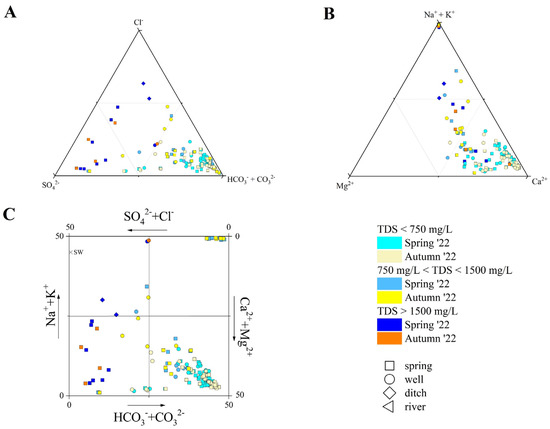
Figure 2.
(A) Anion ternary diagram, (B) cation ternary diagram, and (C) Langelier–Ludwing square diagram for the investigated waters. Samples are reported based on the type of emission, TDS values, and sampling period. Seawater (S.W) composition after [87] is also reported.
Among major cations (Figure 2B), Ca2+ was dominant in springs and wells characterized by relatively low TDS (<1000 mg/L), and in some high-TDS (>1500 mg/L) springs (i.e., NC-26, NC-27, IZ-12, IZ-13, IZ-14, and NB-10), while the (Na+ + K+)-component showed an increase with the TDS. Sodium was the main cation in the sulfur springs, ditches (namely, NB-04 and CZ-05), and IZ-10, IZ-11, IZ-12 wells. The remaining waters (e.g., BS-01, IZ-16) showed an almost equal stoichiometric balance (in meq/L) between the (Na+ + K+)- and (Ca2+ + Mg2+) components. Magnesium concentrations ranged from 0.6 to 185 mg/L in spring, and from 0.5 to 186 mg/L in autumn, with the higher contents measured for the high-TDS springs. Potassium content was generally <5 mg/L, setting aside the high-TDS springs and wells, where it ranged from 14 to 28 mg/L in spring and from 21 to 27 mg/L in autumn, respectively. Anomalously high K+ contents were measured for CZ-01 (35 in spring and 39 mg/L in autumn) and CZ-02 (66 in spring and 68 mg/L in autumn).
Summarizing, the PU waters showed a wide compositional variability, and they were classified following the Langelier–Ludwing square diagram (Figure 2C), as follows: (i) Ca-HCO3 waters, including most of the samples, i.e., those collected from springs and wells characterized by TDS values < 750 mg/L, and the river (BS-05); (ii) Ca-HCO3(SO4) waters, including samples NC-12, NC-16, NC-19, and NC-24, which showed significant enrichment in SO42− (up to 200 mg/L); (iii) Ca-SO4 waters, including high-TDS (>1500 mg/L) springs (i.e., NC-26, NC-27, IZ-13, IZ-14, IZ-15, and NB-10); (iv) Na-HCO3 waters, pertaining to waters collected from sulfur springs (namely NC-28, NC-30, NB-06, NB-09, and NB-10); and (v) Na-Cl waters, those collected from ditches (NB-04 and CZ-05).
Furthermore, as highlighted by the sample distribution in Figure 2C, not all the waters showed well-defined compositional facies: mineral waters BS-01 and IZ16 showed an almost equal content (in meq/L) of both Cl− and SO42− and (Ca2+ + Mg2+) and (Na+ + K+); IZ-12 showed a Na-(Ca)-HCO3-Cl composition; IZ-11 displayed a predominant Na-HCO3 character but with HCO3− = (SO42− + Cl−); hence, it was not comparable to sulfur springs. All the samples maintained the same composition during spring and autumn, with two exceptions: (a) CS-03, which turned from a Ca-HCO3 to Na-(Ca)-Cl-(HCO3); (b) IZ-10, which changed from a Na-SO4-HCO3 to Na-Ca-SO4 composition.
Moreover, ammonium was detected in 65 samples during spring 2022 and in 30 during autumn 2022. The NH4+ content was generally below 0.2 mg/L, with values higher than 1 mg/L detected in sulfur and high-TDS samples with peaks of 22.2 mg/L, in spring, and 18.9 mg/L, in autumn. Strontium concentrations ranged from 0.5 to 12.2 mg/L in spring, and from 0.6 to 12.0 mg/L in autumn, increasing with TDS and showing peak values in Ca- and SO4-rich waters (Figure 2C). Eventually, SiO2 spanned from <1 to 51 mg/L.
The δ18O values varied from −12.05‰ to −4.55‰ V-SMOW in spring and from −10.84‰ to −5.38‰ V-SMOW in autumn, while those of δ2H were between −65.5‰ and −23.11‰ V-SMOW (spring) and between −63.4‰ and −36.9‰ V-SMOW (autumn). As far as the rainwater samples are concerned (Table 1), the δ2H values ranged from −92.6‰ to −11.4‰ V-SMOW, and those of δ18O were from −14.25‰ to −3.35‰ V-SMOW.

Table 1.
Rain sample characteristics. ID, geographic location (in UTM-33N WGS 84 coordinates), altitude (in m above sea level), δ18O-H2O and δ2H-H2O (as the average ± the standard deviation and expressed in ‰ V-SMOW) are reported.
Among the trace elements (Table 2), B ranged from 6 to 4010 μg/L, showing a strong increase with TDS and with the highest values measured for the sulfur and highly saline waters. Aluminum showed the strongest variability between spring and autumn sampling surveys, spanning from 1 to 100 μg/L in spring, with higher values measured for IZ-14, while in autumn it ranged from 6 to 580 μg/L regardless of the sample type. Lithium, Mn, Fe, and As showed the highest concentrations in Ca-SO4 springs. The maximum values for Li were 421 μg/L (BS-01) in autumn and 332 μg/L (NC-27) in spring, with the Na-HCO3 waters being characterized by Li contents generally above 50 μg/L, whereas the CaHCO3 waters rarely had Li exceeding 20 μg/L. Manganese peak values were 625 (IZ-16) and 210 μg/L (IZ-14) in spring and autumn, respectively, while 320 (IZ-15) and 380 μg/L (IZ-14) were those of Fe. Both Mn and Fe showed higher abundances in autumn 2022 but their variability was less influenced by the water composition since high values were also measured in low-salinity springs and wells, e.g., NC-24 showed an Fe content above 200 μg/L and IZ-03 a Mn concentration above 300 μg/L. Arsenic contents were generally below 1 μg/L for most of the samples, setting aside the Ca-SO4 springs showing contents higher than 10 μg/L, i.e., BS-01 (21 μg/L) and NC-27 (16 μg/L). Vanadium, Cr, Cu, Ni, Co, and Zn showed extreme variability during both sampling surveys, as reported in Table 2 and in SM1, and no significant relationship between their contents and the water composition was shown. Selenium concentrations were extremely low or undetectable for most waters, expect for IZ-04 (11.8 μg/L), IZ-18 (14.7 μg/L), and IZ-01 (>20 μg/L in both samplings). Rubidium rarely exceeded 5 μg/L in most of the waters, with the maximum values being detected for samples NC-27 (18 and 34 μg/L) and BS-01 (31 and 22 μg/L). Barium varied from 12 to 780 μg/L in spring, and from 11 to 1030 μg/L in autumn, showing no relationship with the water character. Lead contents were rarely above 1 μg/L and reached the highest values of 2.4 (IZ-07) in spring and 3.5 μg/L (NC-27) in autumn. Cesium showed low contents, generally below 0.01 μg/L, with the only exception of samples NC-27 (8.1 μg/L) and BS-01 (1.4 μg/L).
Table 2.
Main statistical descriptive parameters for trace elements in the investigated waters: N (number of observations), min (minimum), max (maximum), avg (mean), median, Q1, Q3, and s (standard deviation). All values are reported in μg/L. B and Cs determinations were only carried out following the autumn survey.
4.2. Dissolved Gases Chemical and Isotopic Composition
The chemical composition determination (CO2, N2, CH4, O2, Ar, and He) of dissolved gases was carried out on 31 selected sampling points, as follows (Table 3): 16 in both spring and autumn 2022, 11 only in spring 2022, 2 only in autumn 2022 and 2 only in winter 2023. The δ13C-CO2 and δ13C-CH4 values were determined in 17 samples in February 2023. The full results are reported in Table 3. The selected samples were chosen based on the different water compositions, location, and geological context to cover as much as possible the variability of these features.
Table 3.
Chemical and isotopic composition of dissolved gases. CO2, CH4, N2, O2, Ar, and He are reported in mmol/L, whereas δ13C-CO2 and δ13C-CH4 are expressed as ‰ V-PDB. “n.d.” indicates that the value was not detected due to low concentrations. Water chemistry and type of emission (s: spring; w: well; d: ditch) are also reported.
All gases (except that associated with the BS-01, NB-08, and NB-09 samples) were N2-dominant (ranging from 0.31 to 0.76 mmol/L) (Figure 3) with lower concentrations of CO2 (ranging from 0.04 to 0.31 mmol/L), CH4 (ranging 0.004 to 0.024 mmol/L), Ar (ranging from 0.008 to 0.019 mmol/L), and O2 (ranging from 0.005 to 0.28 mmol/L). Helium was the least abundant, ranging from 8 × 10⁻⁶ to 3.2 × 10⁻⁵ mmol/L. The BS-01 (Na(Ca)-SO4(Cl) type), NB-08 (Na-HCO3 type), and NB-09 (Na-HCO3 type) samples were CO2(CH4)-dominant, showing the sum of CO2 (ranging from 0.24 to 0.41 mmol/L) and CH4 (ranging from 0.31 to 0.43 mmol/L) to be higher than N2 (ranging from 0.31 to 0.43 mmol/L) concentrations. In these gases, Ar and O2 ranged from 0.008 to 0.011 mmol/L and from 0.013 to 0.016 mmol/L, respectively. Methane contents showed a slight increase in spring with respect to autumn, while no evident seasonal change was observed for the other gases.
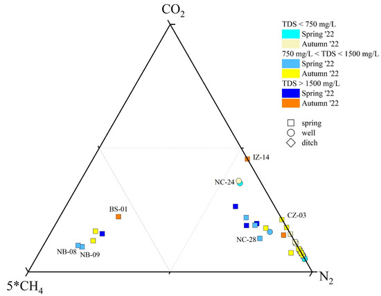
Figure 3.
5*CH4-CO2-N2 ternary diagram for the dissolved gas phase classification. ID as reported in SM1.
The δ13C-CO2 and δ13C-CH4 values were from −11.5 to −74.0‰ and from −27.5 to −68.2‰ vs. V-PDB, respectively. The lowest values of δ13C-CH4 were measured in the sulfur springs, while no clear relationships were observed for the δ13C-CO2 values with the water character and water type.
5. Discussion
5.1. Local Meteoric Water Line and Water Recharge Origin
Rainwater samples were collected on a monthly basis at different altitudes, from 14 to 1267 m above sea level (Table 1), in order to construct a local meteoric water line and have a better understanding of the water recharge and circulation paths feeding springs and wells in the PU province.
Based on the δ2H and δ18O values of the rainwater samples (detailed results are reported in the Supplementary Materials), the local meteoric water line (hereafter, Pesaro-Urbino Meteoric Water Line, PUMWL) was calculated using a best-fit linear function (Equation (1)) obtaining a correlation coefficient (R2) higher than 0.94, confirming the good spatial and vertical distribution of the rain samplers within the study area [88] (Figure 4a):
PUMWL: δ2H = 6.8098xδ18O + 7.7016
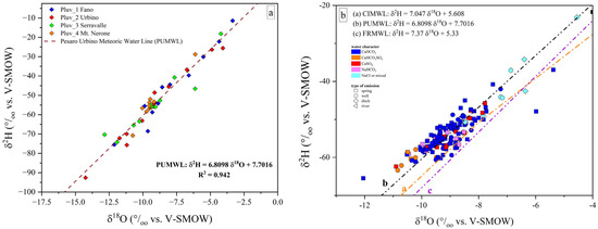
Figure 4.
(a) Binary diagram δ2H vs. δ18O, where the isotopic values measured in the rain samplers (P1-P4) from January 2023 to January 2024 are reported. The dashed black line represents the local meteoric water line (Pesaro-Urbino Meteoric Water Line, PUMWL) computed for the study area. The PUMWL equation and correlation coefficient (R2) are also reported; (b) binary diagram δ2H vs. δ18O for the investigated samples, where the Central Italy Meteoric Water Line (a, CIMWL; [89]), the Pesaro-Urbino Meteoric Water Line (b, PUWML) and the Furlo Ridge Meteoric Water Line (c, FRMWL; [88]) are drawn. δ2H vs. δ18O expressed in ‰ (vs. V-SMOW).
The new computed local Meteoric Water Line shows a different slope with respect to those previously computed such as the Central Italy Meteoric Water Line (CIMWL), e.g., [89,90], and the recently presented Marche Region and Furlo Ridge Meteoric Water Line (FRMWL) [88]. The FRMWL was computed using isotopic data related to the time interval 2013 and 2017. When compared to the present study, the δ2H/δ18O reported by [88] is slightly higher (7.37 vs. 6.81) while the δ2H-intercept is lower (5.33 vs. 7.70).
Most of the investigated waters plot between both the Central Italy Meteoric Water Line (CIMWL; [89]) and PUMWL (Figure 4b). Therefore, the PU waters, besides having a clear meteoric origin, did not show any evidence of 18O enrichment typical of waters affected by water–rock interaction processes at relatively high temperatures. Water samples from ditches showed fewer negative isotopic values compared to those from wells and springs, with the former having been affected by evaporation processes and limited water recharge.
5.2. Processes Governing the Water Composition
The wide compositional variability and large variation in TDS values of the waters discharging in the PU province suggest that springs and wells of this study are fed by different hydrological systems involving distinct and various rocks formations. The different types of waters will be further discussed according to their geochemical facies, as reported in Figure 2, in the following subparagraphs.
5.2.1. Ca-HCO3 and Ca-HCO3(SO4) Waters
The Ca-HCO3-type waters, showing neutral to slightly alkaline pH, positive Eh values, and low-to-medium TDS (from 268 to 1400 mg/L), likely pertain to shallow hydrological circuits, e.g., [85,91]. Generally speaking, their composition is related to the congruent dissolution of carbonate-bearing minerals (Figure 5), mainly calcite and, subordinately, dolomite, that widely occur all over the study area, although slight enrichments in earth alkaline ions indicate the occurrence of alteration processes involving other mineral phases, e.g., Al-silicates, in accordance with the slight excess in Na with respect to Cl shown by these waters (Figure 6a,b). In detail, waters collected from the Mt. Nerone–Mt. Catria Ridge (NC) are marked by low contents of Cl, SO4, NO3, and Na, suggesting that the water–rock interaction only involved carbonates and had a minimal influence of anthropogenic activities. These waters, emerging at a relatively high altitude (>500 m a.s.l), are possibly related to a short hydrological pathway within the Maiolica and Calcare Massiccio calcareous aquifers (Figure 1) [40]. Samples from the Furlo Gorge (FU), Cesane Ridge (CS), and the Northern Border (NB) areas display slight enrichments in chloride, sulfate, boron, and sodium relative to the NC waters (SM1), probably related to silicate weathering (Figure 7a) since these waters circulate and emerge from marly and silicate formations (i.e., Scaglia Fms, Schlier Fm, and Marnoso Arenacea Fm) (Figure 1). Moving east through the Internal Zone (IZ) and Coastal Zone (CZ) (Figure 1), the Ca-HCO3 waters have a general increase in TDS values, mostly linked to the enrichment in NO3 (up to 95 mg/L in the Coastal Zone), locally exceeding the quality target for drinking waters (limit 50 mg/L; e.g., [92]). The enrichments in chloride, sulfate, and potassium shown by waters collected between Fossombrone and Fano (Figure 1) can likely be related to anthropogenic sources, such as agriculture practice (fertilizers) and nursery activity, e.g., [93,94], which are widely diffused in this area [85,86].

Figure 5.
Binary diagram (Ca2+ + Mg2+) vs. (HCO3− + CO32−), both expressed in meq/L. ID as reported in SM1.
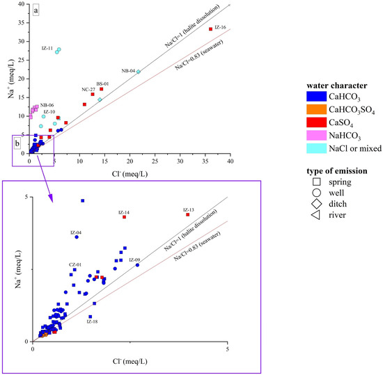
Figure 6.
(a) Binary diagram Na+ vs. Cl−, both expressed in meq/L; (b) distributions of samples with lower Na and/or Cl concentrations. ID as reported in SM1.
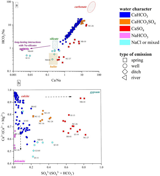
Figure 7.
(a) HCO3/Na vs. Ca/Na binary diagram, values reported as molar ratios. The carbonate, halite, and silicate fields are also reported after [95]. (b) Ca/(Ca + Mg) vs. SO4/(SO4 + HCO3) binary diagram. Existence fields for calcite, dolomite, and gypsum are also reported after [96]. IDs as reported in SM1.
Two springs (NC-12, NC-19) and two wells (NC-16, NC-24), emerging from the Mt. Nerone–Mt. Catria Ridge, are Ca-HCO3-SO4 despite the fact that this area is dominated by Ca-HCO3 waters. In the Burano Valley, the aquifer feeding the NC-16 and NC-24 wells (Figure 1) is intercepted at depths between 125 and 260 m. These samples show slightly alkaline pH, low contents of Cl and Na, higher levels of Mg compared to other NC waters, and strong enrichments of SO4 (up to 215 mg/L), although no peculiar enrichments in trace element contents were recorded (SM1). Thus, the variable sulfate enrichment occurring in this water type suggests deeper and longer hydrological pathways of the meteoric waters and their interaction with the Triassic evaporitic Burano Fm (Figure 7b). The wide variability in SO4 contents shown by the NC-12, NC-16, NC-19, and NC-24 samples (from 70 to 210 mg/L) is likely a consequence of different degrees of interaction with the Burano Fm, which also depend on both the length of the circulation paths and depth of the top of the Triassic evaporites [40].
5.2.2. Ca-SO4 Waters
The Ca-SO4 types are characterized by TDS values of up to 4900 mg/L. Based on their chemical–physical features, these waters are conveniently subdivided into two groups: (1) NC-27, BS-01, IZ-13, IZ-14, IZ-15, and IZ-16 samples, showing a neutral-to-slightly acid pH, negative Eh values, and high Na+, Cl−, and NH4+ contents, with their emergence sites being also characterized by a H2S odor and colloidal elemental sulfur; (2) NC-26 and NB-10 samples, with an almost neutral pH, positive Eh, and low contents of other major elements. The latter showed the same composition and almost equal concentrations in both surveys (spring and autumn). Contrarily, NC-27 and IZ-14 showed a TDS increase while BS-01 decreased (SM1). Furthermore, NC-26 and NB-10 are characterized by low-to-moderate Li and B contents; contrarily, NC-27, BS-01, IZ-13, IZ-14, IZ-15, and IZ-16 show strong enrichments in Li and B as well as relatively high contents of Fe, Mn, Rb, and As. The origin of the Ca-SO4 waters is related to interaction with gypsum–anhydrite lithologies (Figure 7b), i.e., the Burano Fm or the Gessoso-Solfifera Fm, with a variable contribution from halite (and carbonate) dissolution. Specifically, the gypsum–anhydrite dissolution is predominant in NC-26 and NB-10 waters with a minor contribution from halite dissolution due to the low contents of Cl, Na, B, and Li (SM1). Considering the geology of the area (Figure 1), NB-10 probably circulates within the Messinian gypsums, at relatively shallow depths since NO3, typically considered a tracer of anthropogenic contributions, was relatively high (30 mg/L), whereas for NC-26, a contribution from the interaction with the Triassic Burano Fm can be inferred. The NC-26 water probably pertains to the same circulation paths proposed for the Ca-HCO3-SO4 waters, but it shows a higher contribution from gypsum–anhydrite dissolution.
The enrichments in chloride and sodium shown by Ca(Na)-SO4(Cl) waters indicate halite dissolution as another major process governing the geochemistry of these waters (Figure 7a), which is also consistent with their Br, B, and Li contents (SM1). These waters emerge in areas where Messinian evaporites or Triassic anhydrites do not outcrop, thus suggesting that they are related to long flow paths in deeper layers, as highlighted by previous studies [38,97,98].
5.2.3. Na-HCO3 Waters
This water type shows strong Na and HCO3 + CO3 excesses relative to the stoichiometric ratio with Cl and Ca + Mg, respectively (Figure 5 and Figure 6), e.g., [83,84]. Among minor and trace elements, these waters display high contents of F, NH4, Li, and B and relatively low values of Sr and Ba (Figure 8a). Moreover, the B/Cl and Li/Cl ratios in these waters are higher than those recorded in Ca(Na)-SO4(Cl) discharges, indicating that the Na-HCO3 waters are enriched in B and Li (Figure 8b,c) and Cl poor when compared to those detected in the Ca(Na)-SO4(Cl) springs.
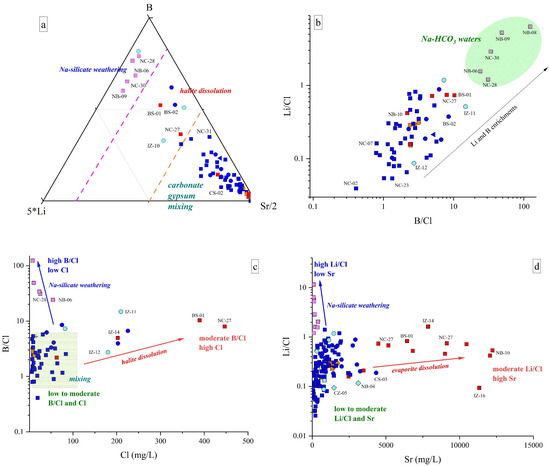
Figure 8.
(a) 5*Li-B-Sr/2 ternary diagram for the investigated waters; (b) Li/Cl v. B/Cl binary diagram. Na-HCO3 water field is also reported; (c) B/Cl vs. Cl (in mg/L) binary diagram; (d) Li/Cl vs. Sr (in μg/L) binary diagram. Symbols as reported in Figure 2. IDs as reported in SM1. Only samples collected in November 2022 are reported in (a–c). Major processes influencing water chemistry are also drawn (i.e., arrows and shaded blocks). IDs as reported in SM1. Symbols and colors as reported in Figure 7.
The occurrence of Na-HCO3 waters is generally associated with the presence of tectonic contacts or alignments, e.g., [83,84,99], and their origin is still debated and possibly related to (a) prograde Na-Ca ionic exchange involving Na-rich clay with consequent release of Na into the solution and the removal of Ca and Mg [83,84,100] or (b) long-lasting interaction and dissolution of plagioclase-rich silicate phases [83,99] in conditions of saturation/oversaturation for carbonate-bearing minerals causing the depletion of Ca, Mg (Figure 5) and, secondarily, of Sr (Figure 8d). The waters emerge from the siliciclastic Marnoso Arenacea Fm, where clay components can be easily found [101] and Na-Ca exchange reactions may occur, e.g., [102]. Nevertheless, as already pointed out by several authors, e.g., [83,84], this process alone is not able to produce enrichments in F, Li, and B and/or alkaline pH values. Contrarily, prolonged interactions between meteoric solutions and Na-rich silicate rocks can generate an alkaline hydrolysis, releasing OH− into the solution, which leads to a considerable pH and Na increase [83,84]. Silicate weathering may explain the high concentrations of Li, B, and F, since they show a particular geochemical affinity with silicate mineral phases and can be found in silicate rocks in considerable contents, e.g., apatite and fluorite [103]. This is further supported by their increase with sodium (0.70 < r < 0.91) (SM2). However, the influence of Na-Ca ionic exchange, to some extent, cannot be excluded [102].
On the other hand, the enrichments of dissolved carbon species shown by Na-HCO3 waters may be produced following the formation of CO2(gas), from organic matter decay according to reactions (1) to (3), which is then converted in HCO3(aq):
- 2CH2O (organic matter) + SO42− + 2H+ → 2CO2 + H2S + 2H2O;
- 2CH2O (organic matter) + SO42− → H2S + 2HCO3−;
- CH4 + SO42− → HS− + HCO3− + H2O.
The release of CO2(gas) into the solution also favors silicate weathering, e.g., [102]. These reactions determine the production of H2S, e.g., [83,84,104], which was not analytically determined but clearly sniffed and consistent with the Eh values and CO2 and CH4 contents measured in these samples. The Na-HCO3 springs, as well as those with Ca(Na)-SO4(Cl) composition (i.e., NC-27, BS-01, IZ-13, IZ-14, IZ-15, and IZ-16) have Eh values pertaining to reducing environments as also suggested by the relatively high contents of ammonia. Consequently, these waters are likely circulating within organic matter-rich layers that can be found in both the silicate and evaporitic formations [51,73] and are associated with longer and deeper hydrological pathways.
5.2.4. Na-Cl and Waters with Mixed Composition
The ditch waters, i.e., NB-04 and CZ-05, both flowing on the clay formation of the Argille Azzurre, were characterized by a Na-Cl character. They showed high values of TDS (2332 mg/L, NB-04; 1773; CZ-05), high contents of sulfate (up to 256 mg/L) and calcium (up to 169 mg/L), and variable contents of minor elements (SM1). IZ-05 is also related to a ditch, but due to the high turbidity of the water, it was only sampled for water isotopes and dissolved gases. Their composition is generally consistent with dissolution processes of evaporitic minerals that, however, do not outcrop in the surrounding areas. Accordingly, they probably originate from mixing processes between meteoric and highly saline waters with Na-Cl-(SO4) composition, the latter being found within the clayey foredeep deposits, as also reported by [97,98].
IZ-10 and IZ-11 belong to the same well, having been collected at the top and bottom of it, and have an almost equal balance of (HCO3 + CO32−)- and (Cl + SO4) components, with HCO3 > SO4 > Cl in IZ10 and HCO3 = Cl >> SO4 in IZ-11, Na as the predominant cation, moderate Li, and high B contents. Similar features were also found in the IZ-12 sample. The complex composition shown by these waters suggests the occurrence of different water–rock interaction processes, including (i) dissolution of calcite and evaporite minerals, and (ii) silicate weathering. Moreover, mixing between surface and Na-Cl-(SO4) fossil waters cannot be ruled out [97,98].
5.3. Origin of Dissolved Gases
The origin of dissolved gas species in surface waters, springs, and shallow groundwaters is generally ascribed to (i) dissolution of atmospheric gases, (ii) biogeochemical processes in the water body and water–sediment interfaces, and (iii) deep-sourced gas contributions [79,105,106,107]. The N2, Ar, and O2 contents in both N2- and CO2(CH4)-dominated samples are related to the occurrence of atmospheric gases, as shown by the distribution of the water samples in the triangular N2-Ar-O2 plot (Figure 9), where the investigated waters plot along the alignment between the composition of ASW (Air-Saturated Water) and O2-depleted ASW, within the ASW domain (38 < N2/Ar < 42). The relative depletion of O2 with respect to the other air-related components is not surprising, given that O2 is highly reactive and enters several biochemical reactions as an electron acceptor. Shedding light on the origin of CH4 and CO2 appears instead more challenging since these species undergo several physicochemical processes, which at a shallow depth are mostly driven by different microbial communities, which are prone to metabolize preferentially the lighter C atoms [108,109]. The δ13C-CO2 and δ13C-CH4 values are generally considered the best tools to obtain insights into the sources of these C-bearing species [105,106,107].
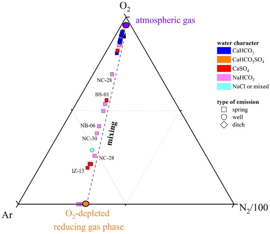
Figure 9.
Ar-N2-O2 ternary diagram for the dissolved gases samples. The mixing line between atmospheric gases and an O2-depleted reducing gas phase is reported. IDs as reported in SM1.
Most of the N2-dominated water samples fell within the microbial field, as shown in Figure 10, suggesting that CO2 and CH4 are biogenic, produced by plant-root respiration and/or anaerobic decay of organic matter trapped into sediments mediated by SO4 (e.g., reaction (1)) or methane-producing microorganisms [108,109], with a slight influence of secondary process in modifying the isotopic signatures, e.g., [107]. The CO2(CH4)-dominated NB-09 seems to be too enriched in 13C-CO2 to fall in the microbial field: such a 13C-enrichment may be caused by CO2 microbial consumption, a process leading to 13C-CO2 enrichment in the residual gas phase [106,110]. Microbial oxidation of CH4 is probably the reason for the relative enrichment of 12C-CO2 and 13C-CH4 in the N2-dominated NC-27 and the CO2(CH4)-dominated BS-01 samples: during CH4 oxidation, microbes preferentially degrade 12C-CH4 to produce CO2 relatively enriched in 12C [111,112]. Moreover, the apparent thermogenic contribution observed for CH4 in the N2-dominated NB-07 and NC-19 samples (Figure 10) might be due to the strong microbial methane oxidation favored by oxidizing conditions (positive Eh values) [106]. In conclusion, the isotopic data indicate that CO2 and CH4 are produced at relatively shallow depths following different biogeochemical processes. According to the geological background and geodynamic setting of the study area, the influence of deep-originated fluids in the shallow aquifers may be ruled out or considered negligible, e.g., [113,114].
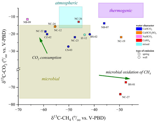
Figure 10.
δ13C-CO2 vs. δ13C-CH4 (both expressed in ‰ vs. V-PDB) binary diagram. The boxes report the average carbon isotopic ratios for the different genetic processes: biogenesis, thermogenesis, and dissolution of atmospheric gases. The green arrows represent the most common secondary processes (i.e., CO2 consumption, CH4 microbial oxidation) that may influence the isotopic composition. Reference values for δ13C from [106,110]. IDs as reported in SM1.
6. Conclusions and Future Perspectives
The development of a multiparametric water monitoring network aimed at seismic surveillance and sustainability requires the selection of sampling sites suitable to record possible changes related to an impending event, and for this purpose, a detailed and wide geochemical characterization is a crucial and demanding step. The results presented in this work can be regarded as background values established prior to future earthquakes and also as the basis for deploying a geochemical monitoring network in the seismically active area of the Pesaro-Urbino province. According to our study, Ca-HCO3(SO4), Ca(Na)-SO4(Cl), and Na-HCO3 water discharges are likely related to relatively deeper hydrogeological pathways, and their emergence at the surface is probably favored by the local structures (i.e., faults, tectonic alignments). Additionally, they also appear to be less influenced by external contributions (i.e., anthropogenic activities, the dissolution of atmospheric gases). Hence, the above hydrochemical compositional facies can be considered the most suitable to be included in a monitoring network for geochemical tracers for earthquakes, which would likely involve an extensive suite of parameters (e.g., major and minor ions, trace elements, and O-H isotopes). Furthermore, since the isotopic composition of dissolved gases clearly suggests an origin related to a shallow biogenic derivation and/or to the dissolution of atmospheric gases (with a negligible influence from deep-seated fluids), the δ13C-CO2 and δ13C-CH4 values may represent interesting and useful parameters to be monitored, since increasing seismic fracturing processes, e.g., [115], may produce significant variations in both the chemical and isotopic gas composition, thus testifying to the uprising of deep fluids, e.g., [12,24,114,116]. Changes in major ion concentrations (i.e., Na, Cl, SO4) as well as in trace element contents (e.g., B, Fe, Cr) of waters cannot be ruled out as promising geochemical tracers of seismic events. Nevertheless, additional hydrological, geochemical, and isotopic analyses are required to better understand the water–rock interaction process and infer the length and depth of the water circulation paths within the study area.
Supplementary Materials
The following supporting information can be downloaded at: https://www.mdpi.com/article/10.3390/su16125178/s1, File S1: Supplementary Material 1; File S2: Supplementary Material 2.
Author Contributions
All authors contributed to the study and manuscript. L.C.: conceptualization, methodology, investigation, validation, formal analysis, data curation, visualization, writing—original draft, writing—review and editing. M.T.: conceptualization, visualization, methodology, investigation, validation, writing—review and editing, supervision. J.C.: investigation, validation, writing—review and editing. F.C.: formal analysis. A.R. (Antonio Randazzo): investigation, formal analysis, writing—review and editing. F.T.: methodology, formal analysis, investigation, writing—review and editing. A.R. (Alberto Renzulli): conceptualization, resources, supervision, writing—review and editing. O.V.: methodology, investigation, resources, supervision, writing—review and editing. All authors have read and agreed to the published version of the manuscript.
Funding
L.C. is financially supported by a ReMeST PhD Grant (XXXVII cycle) financed by the University of Urbino. M.T. is financially supported by a research contract co-financed by the European Union “ESF-REACT-EU, PON Research, and Innovation 2014–2020 DM1062/2021 (grant n. 63-G-19603-1)”.
Data Availability Statement
Data is contained within the article.
Acknowledgments
The authors wish to thank Eng. A. Tiboni and Marche Multiservizi (MMS) S.p.A for granting access to the Pesaro-Urbino aqueduct network and MMS technicians (G. Piergiovanni, A. Lucarelli, M. Fanelli, G. Pezzolesi) for their support during fieldwork. The staff of Rifugio Corsini, Casa Archilei, Osservatorio Serpieri, and F. Pezzaglia are also thanked for allowing us to place rain samplers on their properties. C. Maccelli is warmly thanked for analytical support. Finally, we would also like to thank the locals who provided us with help and support in finding and locating some springs. The authors thank N. Voltattorni, who handled the Special Issue “Active Tectonic, Geological Hazard and Seismic Sustainability”. The four anonymous reviewers are thanked for their suggestions and hints, which helped us improve the first version of the article.
Conflicts of Interest
The authors declare no conflicts of interest.
References
- Center for Research on the Epidemiology of Disasters (CRED). Economic Losses, Poverty, and Disasters (1998–2017); CRED: Bengaluru, India; Institute of Health and Society (IRSS): Newcastle, UK; The United Nations Office for Disaster Risk Reduction (UNISDR): Geneva, Switzerland, 2018. [Google Scholar]
- Mantovani, E.; Viti, M.; Babbucci, D.; Tamburelli, C.; Vannucchi, A.; Falciani, F.; Cenni, N. Assetto Tettonico e Potenzialità Sismogenetica dell’Appennino Tosco-Umbro-Marchigiano; Università di Siena: Siena, Italy, 2018. [Google Scholar]
- Calamita, F.; Coltorti, M.; Piccinini, D.; Pierantoni, P.P.; Pizzi, A.; Ripepe, M.; Scisciani, V.; Turco, E. Quaternary faults and seismicity in the Umbro-Marchean Apennines (Central Italy): Evidence from the 1997 Colfiorito earthquake. J. Geodyn. 2000, 29, 245–264. [Google Scholar] [CrossRef]
- De Luca, G.; Di Carlo, G.; Tallini, M. A record of changes in the Gran Sasso groundwater before, during and after the 2016 Amatrice earthquake, central Italy. Sci. Rep. 2018, 18, 15982. [Google Scholar] [CrossRef] [PubMed]
- DISS Working Group. Database of Individual Seismogenic Sources (DISS), Version 3.3.0: A Compilation of Potential Sources for Earthquakes Than M 5.5 in Italy and Surrounding Areas; Istituto Nazionale di Geofisica e Vulcanologia (INGV): Sezione di Catania, Italy, 2021. [Google Scholar]
- Rovida, A.; Locati, M.; Camassi, R.; Lolli, B.; Gasperini, P.; Antonucci, A. Italian Parametric Earthquake Catalogue (CPTI15), Version 4.0; Istituto Nazionale di Geofisica e Vulcanologia (INGV): Sezione di Catania, Italy, 2022. [Google Scholar]
- Monachesi, G.; Caselli, V.; Vasapollo, N. Historical earthquakes in Central Italy: Case histories in the Marche area. Tectonophysics 1991, 193, 95–107. [Google Scholar] [CrossRef]
- King, C.-Y. Gas geochemistry applied to earthquake prediction: An overview. J. Geophys. Res. 1986, 91, 12269–12281. [Google Scholar] [CrossRef]
- Thomas, D. Geochemical precursors to seismic activity. Pure Appl. Geophys. 1988, 126, 241–266. [Google Scholar] [CrossRef]
- King, C.-Y.; Basler, D.; Presser, T.S.; Evans, W.C.; Minissale, A. In search of earthquake related hydrologic and chemical changes along Hayward fault. Appl. Geochem. 1994, 9, 83–91. [Google Scholar] [CrossRef]
- Italiano, F.; Caracausi, A.; Favara, R.; Innocenzi, P.; Martinelli, G. Geochemical monitoring of cold waters during seismicity: Implications for earthquake-induced modifications in shallow aquifers. Terr. Atmos. Ocean. Sci. 2005, 16, 709–729. [Google Scholar] [CrossRef]
- Italiano, F.; Martinelli, G.; Nuccio, P.M. Anomalies of mantle-derived helium during the 1997–1998 seismic swarm of Umbria-Marche, Italy. Geophys. Res. Lett. 2001, 28, 839–842. [Google Scholar] [CrossRef]
- Claesson, L.; Skelton, A.; Graham, C.; Dieti, C.; Mörth, C.-M.; Torssander, P.; Kockum, I. Hydrogeochemical changes before and after a major earthquake. Geology 2004, 32, 641–644. [Google Scholar] [CrossRef]
- Cicerone, R.D.; Ebel, J.E.; Britton, J. A systematic compilation of earthquake precursors. Tectonophysics 2009, 476, 371–396. [Google Scholar] [CrossRef]
- Skelton, A.; Andrén, M.; Kristmannsdóttir, H.; Stockmann, G.; Mörth, C.-M.; Sveinbjörnsdòttir, A.; Jónsson, S.; Sturkell, E.; Guorúnardóttir, H.-R.; Hjartarson, H.; et al. Changes in groundwater chemistry before two consecutive earthquakes in Iceland. Nat. Geosci. 2014, 7, 752. [Google Scholar] [CrossRef]
- Skelton, A.; Claesson, L.; Wästeby, N.; Andrén, M.; Stockmann, G.; Sturkell, E.; Mörth, C.-M.; Stefansson, A.; Tollefsen, E.; Siegmund, H.; et al. Hydrochemical changes before and after earthquakes based on long-term measurements of multiple parameters at two sites in Northern Iceland—A review. J. Geophys. Res. Solid Earth 2019, 124, 2702–2720. [Google Scholar] [CrossRef]
- Manga, M.; Wang, C.-Y.; Shirzaei, M. Increased stream discharge after 3 September 2016 Mw 5.8 Pawnce, Oklahoma earthquake. Geophys. Res. Lett. 2016, 43, 11588–11594. [Google Scholar] [CrossRef]
- Sano, Y.; Takahata, N.; Kagoshima, T.; Shibata, T.; Onoue, T.; Zhao, D. Groundwater helium anomaly reflects strain change during the 2016 Kumamoto earthquake in Southwest Japan. Sci. Rep. 2016, 6, 37939. [Google Scholar] [CrossRef]
- Barberio, M.D.; Barbieri, M.; Billi, A.; Doglioni, C.; Petitta, M. Hydrogeochemical changes before and during the 2016 Amatrice-Norcia seismic sequence (central Italy). Sci. Rep. 2017, 7, 11735. [Google Scholar] [CrossRef] [PubMed]
- Barberio, M.D.; Gori, F.; Barbieri, M.; Billi, A.; Caracausi, A.; De Luca, G.; Franchini, S.; Petitta, M.; Doglioni, C. New observations in Central Italy of groundwater responses to worldwide seismicity. Sci. Rep. 2020, 10, 17850. [Google Scholar] [CrossRef] [PubMed]
- Hosono, T.; Yamada, C.; Shibata, T.; Tawara, Y.; Wang, C.-Y.; Manga, M.; Rahman, A.T.M.S.; Shimada, J. Coseismic groundwater drawdown along crustal ruptures during the 2016 Mw 7.0 Kumamoto earthquake. Water Resour. Res. 2019, 55, 5891–5903. [Google Scholar] [CrossRef]
- Hosono, T.; Yamada, C.; Manga, M.; Wang, C.-Y.; Tanimizu, M. Stable isotopes show that earthquakes enhance permeability and release water from mountains. Nat. Commun. 2020, 11, 2776. [Google Scholar] [CrossRef] [PubMed]
- Hosono, T.; Masaki, Y. Post-seismic hydrochemical changes in regional groundwater flow systems in response to the 2016 Mw 7.0 Kumamoto earthquake. J. Hydrol. 2020, 580, 124340. [Google Scholar] [CrossRef]
- Barbieri, M.; Franchini, S.; Barberio, M.D.; Billi, A.; Boschetti, T.; Giansante, L.; Gori, F.; Jónsson, S.; Petitta, M.; Skelton, A.; et al. Changes in groundwater trace element concentrations before seismic and volcanic activities in Iceland during 2010–2018. Sci. Total Environ. 2021, 793, 14863. [Google Scholar] [CrossRef]
- Franchini, F.; Agostini, S.; Barberio, M.D.; Barbieri, M.; Billi, A.; Boschetti, T.; Pennisi, M.; Petitta, M. HydroQuakes, central Apennines: Towards a hydrogeochemical monitoring network for seismic precursors and the hydro-seismo-sensitivity of boron. J. Hydrol. 2021, 598, 125754. [Google Scholar] [CrossRef]
- Lee, H.A.; Hamm, S.-Y.; Woo, N.C. Groundwater monitoring network for earthquake surveillance and prediction. Econ. Environ. Geol. 2017, 50, 401–414. [Google Scholar]
- Lee, H.A.; Hamm, S.-Y.; Woo, N.C. Pilot-scale groundwater monitoring network for earthquake surveillance and forecasting research in Korea. Water 2021, 13, 2448. [Google Scholar] [CrossRef]
- Martinelli, G. Previous, current and future trends in research into earthquake precursors in geofluids. Geosciences 2020, 10, 189. [Google Scholar] [CrossRef]
- Martinelli, G.; Tamburello, G. Geological and geophysical factors constraining the occurrence of earthquake precursors in geofluids. Front. Earth Sci. 2020, 8, 596050. [Google Scholar] [CrossRef]
- Wang, C.-Y.; Manga, M. Water and Earthquakes; Springer Nature: Heidelberg, Germany, 2021. [Google Scholar]
- Doglioni, C.; Barba, S.; Carminati, E.; Riguzzi, F. Fault on-off versus coseismic fluid reactions. Geosci. Front. 2014, 5, 767–780. [Google Scholar] [CrossRef]
- Manga, M.; Rowland, J.C. Response of Alum Rock springs to the October 30, 2007 Alum Rock earthquake and implications for the origin of increased discharge after earthquakes. Geofluids 2009, 9, 237–250. [Google Scholar] [CrossRef]
- Wang, C.-Y.; Manga, M. New streams and springs after the 2014 Mw 6.0 South Napa earthquake. Nat. Commun. 2015, 6, 7597. [Google Scholar] [CrossRef] [PubMed]
- Yasuoka, Y.; Igarashi, G.; Ishikawa, T.; Tokanami, S.; Shinogi, M. Evidence of precursor phenomena in the Kobe earthquake obtained from atmospheric radon concentration. Appl. Geochem. 2006, 21, 1064–1072. [Google Scholar] [CrossRef]
- Fu, C.C.; Yang, T.F.; Tsai, M.C.; Lee, L.C.; Liu, T.K.; Walia, V.; Chen, C.H.; Chang, W.Y.; Kumar, A.; Lai, T.H. Exploring the relationship between soil degassing and seismic activity by continuous radon monitoring in the Longitudinal Valley of eastern Taiwan. Chem. Geol. 2017, 469, 163–175. [Google Scholar] [CrossRef]
- Kitagawa, Y.; Koizumi, N.; Takahashi, M.; Matsumoto, N.; Sato, T. Changes in groundwater levels or pressures associated with the 2004 earthquake off the west coast of northern Sumatra (M9.0). Earth Planets Space 2006, 58, 173–179. [Google Scholar] [CrossRef]
- Sil, S.; Freymueller, J.T. Water level changes in Fairbanks, Alaska, due to the great Sumatra-Andaman earthquake. Earth Planets Space 2006, 651, 232–241. [Google Scholar] [CrossRef]
- Nanni, T.; Vivalda, P. The aquifers of the Umbria-Marche Adriatic region: Relationships between structural setting and groundwater chemistry. Boll.-Soc. Geol. Ital. 2005, 124, 523–542. [Google Scholar]
- Bison, P.; Mariotti, C.; Pieroni, M.; Piovesana, F.; Priante, M.; Pugi, S. Valutazione e protezione delle risorse idriche sotterranee nella dorsale carbonatica Mt. Catria-Mt. Nerone (Marche). Ing. Geol. Degli Acquiferi 1995, 5, 13–24. [Google Scholar]
- Capaccioni, B.; Didero, M.; Paletta, C.; Salvadori, P. Hydrogeochemistry of groundwaters from carbonate formations with basal gypsiferous layers: An example from the Mt. Catria-Mt. Nerone ridge (Northern Apennines, Italy). J. Hydrol. 2001, 253, 14–26. [Google Scholar] [CrossRef]
- Capaccioni, B.; Nesci, O.; Sacchi, E.M.; Savelli, D.; Troiani, F. Caratterizzazione idrochimica di un acquifero superficiale: Il caso della circolazione idrica nei corpi di frana nella dorsale carbonatica di M. Pietralata—M. Paganuccio (Appennino Marchigiano). Il Quat. 2004, 17, 585–595. [Google Scholar]
- Centamore, E.; Chiocchini, M.; Deiana, G.; Micarelli, A.; Pieuriccini, U. Contributo alla conoscenza del Giurassico dell’Appennino umbro-marchigiano. Studi Geol. Camerti 1971, 1, 7–89. [Google Scholar]
- Centamore, E.; Deiana, G.; Micarelli, A.; Potetti, M. Il Trias-Paleogene delle Marche. In Studi Geologici Camerti, Volume Speciale “La Geologia delle Marche”; Università di Camerino: Camerino, Italy, 1986; pp. 7–27. [Google Scholar]
- Centamore, E.; Fumanti, F.; Nisio, S. The Central-Northern Apennines geological evolution from Triassic to Neogene time. Boll. Soc. Geol. Ital. 2002, 121, 181–197. [Google Scholar]
- Centamore, E.; Micarelli, A. Stratigrafia. In L’Ambiente Fisico delle Marche; Minetti, A., Nanni, T., Perilli, F., Polonara, L., Principi, M., Eds.; Regione Marche, Assessorato Urbanistica e Ambiente: Ancona, Italy, 1991; pp. 5–58. [Google Scholar]
- Capuano, N. Note Illustrative della Carta Geologica d’Italia alla Scala 1:50.000 “Foglio 279—Urbino”; Servizio Geologico d’Italia: Roma, Italy, 2009. [Google Scholar]
- Capuano, N.; Tonelli, G.; Veneri, F. Ricostruzione dell’evoluzione paleogeografica del margine appennino nell’area feltresca (Marche settentrionali) durante il Pliocene Inferiore e Medio. Mem. Soc. Geol. Ital. 1986, 35, 163–170. [Google Scholar]
- Cresta, S.; Monechi, S.; Parisi, G. Mesozoic-Cenozoic Stratigraphy in the Umbria-Marche Area. In Memorie Descrittive della Carta Geologica d’Italia; Servizio Geologico d’Italia: Roma, Italy, 1989; Volume 39. [Google Scholar]
- Barchi, M.; Minelli, G.; Pialli, G. The CROP 03 profile: A synthesis of results on deep structures of the Northern Apennines. Mem. Soc. Geol. Ital. 1998, 52, 383–400. [Google Scholar]
- Barchi, M.; Landuzzi, A.; Minelli, G.; Pialli, G. Outer Northern Apennines. In Anatomy of an Orogen, the Apennines and Adjacent Mediterranean Basins; Vai, G.B., Martini, I.P., Eds.; Kluwer Academic Publishers: Dordrecht, The Netherlands, 2001; pp. 215–254. [Google Scholar]
- Conti, P.; Cornamusini, G.; Carmignani, L. An outline of the geology of the Northern Apennines (Italy), with geological map 1:250,000 scale. Ital. J. Geosci. 2020, 139, 149–194. [Google Scholar] [CrossRef]
- Meyer, L.; Menichetti, M.; Nesci, O.; Savelli, D. Morphotectonic approach to the drainage analysis in the North Marche region, central Italy. Quat. Int. 2003, 101–102, 157–167. [Google Scholar] [CrossRef]
- Lavecchia, G.; Boncio, P.; Creati, N. A lithospheric-scale seismogenic thrust in Central Italy. J. Geodyn. 2003, 36, 79–94. [Google Scholar] [CrossRef]
- Lavecchia, G.; Barchi, M.; Brozzetti, F.; Menichetti, M. Sismicità e tettonica nell’area umbro-marchigiana. Boll. Soc. Geol. Ital. 1994, 113, 483–500. [Google Scholar]
- Boncio, P.; Brozzetti, F.; Lavecchia, G. Architecture and seismotectonics of regional low-angle normal fault zone in Central Italy. Tectonics 2000, 19, 1038–1055. [Google Scholar] [CrossRef]
- Boncio, P.; Brozzetti, F.; Ponziani, F.; Barchi, M.; Lavecchia, G.; Pialli, G. Seismicity and extensional tectonics in the Northern Umbria-Marche Apennines. Mem. Soc. Geol. Ital. 1998, 52, 539–555. [Google Scholar]
- De Donatis, M.; Alberti, M.; Cipicchia, M.; Munoz-Guerrero, N.; Pappafico, G.F.; Susini, S. Workflow of digital field mapping and drone-aided survey for the identification and characterization of capable faults: The case of normal fault system in the Mt. Nerone area (Northern Apennines, Italy). Int. J. Geo-Inf. 2020, 9, 616. [Google Scholar] [CrossRef]
- Mazzoli, S.; Machiavelli, C.; Ascione, A. The 2013 Marche off-shore earthquakes: New insights into the active tectonic setting of the outer-northern Apennines. J. Geol. Soc. 2014, 171, 457–460. [Google Scholar] [CrossRef]
- Mazzoli, S.; Pierantoni, P.P.; Borraccini, F.; Paltrinieri, W.; Deiana, G. Geometry, segmentation pattern and displacement variations along a major Apennine thrust zone, central Italy. J. Struct. Geol. 2005, 27, 1940–1953. [Google Scholar] [CrossRef]
- Mazzoli, S.; Santini, S.; Macchiavelli, C.; Ascione, A. Active tectonics of the outer Northern Apennines: Adriatic vs. Po Plain seismicity. J. Geodyn. 2015, 84, 62–76. [Google Scholar] [CrossRef]
- Pierantoni, P.P.; Chicco, J.; Costa, M.; Invernizzi, C. Plio-Quaternary transpressive tectonics: A key factor in the structural evolution of the outer Apennine-Adriatic system, Italy. J. Geol. Soc. 2019, 176, 1273–1283. [Google Scholar] [CrossRef]
- Maesano, F.E.; Buttinelli, M.; Maffucci, R.; Toscani, G.; Basili, R.; Bonini, L.; Burrato, P.; Fedorik, J.; Fracassi, U.; Panara, Y.; et al. Buried alive: Imaging of the 9 November 2022, M2 5.5 earthquake source on the Offshore Adriatic blind thrust front of the Northern Apennines (Italy). Geophys. Res. Lett. 2023, 50, e2022GL102299. [Google Scholar] [CrossRef]
- Pezzo, G.; Billi, A.; Carminati, E.; De Gori, P.; Devoti, R.; Lucente, F.P.; Palano, M.; Petracchini, L.; Serpelloni, E.; Tavani, S.; et al. Seismic source of identification of the 9 November 2022 Mw 5.5 offshore Adriatic Sea (Italy) earthquake from GNSS data and aftershock relocation. Sci. Rep. 2023, 13, 11474. [Google Scholar] [CrossRef] [PubMed]
- Anelli, L.; Gorza, M.; Pieri, M.; Riva, M. Subsurface well data in the northern Apennines (Italy). Mem. Soc. Geol. Ital. 1994, 48, 461–471. [Google Scholar]
- Martinis, B.; Pieri, M. Alcune notizie sulla formazione evaporitica del Triassico superiore nell’Italia centrale e meridionale. Mem. Soc. Geol. Ital. 1964, 4, 649–678. [Google Scholar]
- Barchi, M.R.; De Feyter, A.; Magnani, M.B.; Minelli, G.; Pialli, G.; Sotera, B.M. The structural style of the Umbria-Marche fold and thrust belt. Mem. Soc. Geol. Ital. 1998, 52, 557–578. [Google Scholar]
- VIDEPI Project. 2009. Available online: https://www.videpi.com (accessed on 1 March 2024).
- Donatelli, U.; Tramontana, M. Platform-to-basin facies transition and tectono-sedimentary processes in the Jurassic deposits of the Furlo area (Umbria-Marche Apennines, Italy). Facies 2013, 60, 541–560. [Google Scholar] [CrossRef]
- Donatelli, U.; Tramontana, M. Jurassic carbonate depositional systems of the Mt. Catria-Mt. Acuto area (Umbria-Marche Apennines, Italy). Ital. J. Geosci. 2012, 131, 3–18. [Google Scholar] [CrossRef]
- Santantonio, M. Facies associations and evolution of pelagic carbonate platform/basin systems: Examples from the Italian Jurassic. Sedimentology 1993, 40, 1039–1067. [Google Scholar] [CrossRef]
- Ricci Lucchi, F. The Oligocene to recent foreland basins of the Northern Apennines. In Foreland Basins; Allen, P.A., Homewood, P., Eds.; Special Publications; International Association of Sedimentologists: Belgium, Brussel; Blackwell Scientific Publications: Oxford, UK, 1986; Volume 8, pp. 105–139. [Google Scholar]
- Argnani, A.; Ricci Lucchi, F. Tertiary silicoclastic turbidite systems of the Northern Apennines. In Anatomy of an Orogen: The Apennines and Adjacent Mediterranean Basins; Vai, G.B., Martini, I.P., Eds.; Kluwer Academic Publishers: Dordrecht, The Netherlands, 2001; pp. 327–350. [Google Scholar]
- Tavernelli, E. Structural evolution of a foreland fold-and-thrust belt: The Umbria-Marche Apennines, Italy. J. Struct. Geol. 1997, 19, 523–534. [Google Scholar] [CrossRef]
- Nesci, O.; Savelli, D.; Troiani, F. Evoluzione tardo quaternaria dell’area di foce del Fiume Metauro (Marche Settentrionali). In Collana dell’Autorità di Bacino della Basilicata, Proceedings of the Coste: Prevenire, Programmare, Pianificare Conference, Maratea, Italy, 15–17 May 2008; Autorità di Bacino della Basilicata: Potenza, Italy, 2008; Volume 9, pp. 443–451. [Google Scholar]
- Gallerini, G.; De Donatis, M. 3D modeling using geognostic data: The case of the low valley of the Foglia river (Italy). Comput. Geosci. 2009, 35, 146–164. [Google Scholar] [CrossRef]
- Taussi, M.; Borghi, W.; Gliaschera, M.; Renzulli, A. Defining the shallow geothermal heat-exchange potential for a lower fluvial plain of the central Apennines: The Metauro Valley (Marche region, Italy). Energies 2021, 14, 768. [Google Scholar] [CrossRef]
- Morelli, S.; Bonì, R.; Guidi, E.; De Donatis, M.; Pappafico, G.; Francioni, M. L’Alluvione delle Marche del 15 Settembre 2022, cause e conseguenze. In La Dinamica Fluviale. La Conoscenza del Fiume per la Pianificazione e la Salvaguardia del Territorio; Cencetti, C., Di Matteo, L., Eds.; Culture Territori Linguaggi, 2023; Volume 24, pp. 136–147. ISBN 9788894469783. [Google Scholar]
- Gröning, M.; Lutz, H.O.; Roller-Lutz, Z.; Kralik, M.; Gourcy, L.; Pöltenstein, L. A simple rain collector preventing water re-evaporation dedicated for, δ.1.8.O.; δ2H analysis of cumulative precipitation samples. J. Hydrol. 2012, 448–449, 195–200. [Google Scholar] [CrossRef]
- Tassi, F.; Garofalo, P.S.; Turchetti, F.; De Santis, D.; Capecchiacci, F.; Vaselli, O.; Cabassi, J.; Venturi, S.; Vannini, S. Insights into the Porretta Terme (northern Apennines, Italy) hydrothermal system revealed by geochemical data on presently discharging thermal waters and paleofluids. Environ. Geochem. Health 2022, 44, 1925–1948. [Google Scholar] [CrossRef] [PubMed]
- Vaselli, O.; Tassi, F.; Montegrossi, G.; Capaccioni, B.; Giannini, L. Sampling and analysis of volcanic gasses. Acta Vulcanol. 2006, 18, 65–76. [Google Scholar]
- Wilhelm, E.; Battino, R.; Wilcock, R.J. Low-pressure solubility of gasses in liquid waters. Chem. Rev. 1977, 77, 219–262. [Google Scholar] [CrossRef]
- Venturi, S.; Tassi, F.; Cabassi, J.; Gioli, B.; Baronti, S.; Vaselli, O.; Caponi, C.; Vagnoli, C.; Picchi, G.; Zaldei, A.; et al. Seasonal and diurnal variations of greenhouse gases in Florence (Italy): Inferring sources and sinks from carbon isotopic ratios. Sci. Total Environ. 2020, 698, 134245. [Google Scholar] [CrossRef]
- Toscani, L.; Venturelli, G.; Boschetti, T. Sulphide-bearing waters in Northern Apennines, Italy: General features and water-rock interaction. Appl. Geochem. 2001, 7, 195–216. [Google Scholar]
- Venturelli, G.; Boschetti, T.; Duchi, V. Na-carbonate waters of extreme composition: Possible origin and evolution. Geochem. J. 2003, 37, 351–366. [Google Scholar] [CrossRef]
- Nisi, B.; Vaselli, O.; Taussi, M.; Doveri, M.; Menichini, M.; Cabassi, J.; Raco, B.; Botteghi, S.; Mussi, M.; Masetti, G. Hydrogeochemical surveys of shallow coastal aquifers: A conceptual model to set-up a monitoring network and increase the resilience of a strategic groundwater system to climate change and anthropogenic pressure. Appl. Geochem. 2022, 142, 105305. [Google Scholar] [CrossRef]
- Taussi, M.; Gozzi, C.; Vaselli, O.; Cabassi, J.; Menichini, M.; Doveri, M.; Romei, M.; Ferretti, A.; Gambioli, A.; Nisi, B. Contamination assessment and temporal evolution of nitrates in the shallow aquifer of the Metauro River Plain (Adriatic Sea, Italy) after remediation actions. Int. J. Environ. Res. Public Health 2022, 19, 12231. [Google Scholar] [CrossRef] [PubMed]
- Gibbs, R.J. Mechanisms controlling world water chemistry. Science 1979, 170, 1088–1090. [Google Scholar] [CrossRef] [PubMed]
- Tazioli, A.; Fronzi, D.; Palpacelli, S. Regional vs. local isotopic gradient: Insights and modeling from mid-mountain area in Central Italy. Groundwater 2024. [Google Scholar] [CrossRef] [PubMed]
- Longinelli, A.; Selmo, E. Isotopic composition of precipitation in Italy: A first overall map. J. Hydrol. 2003, 270, 75–88. [Google Scholar] [CrossRef]
- Giustini, F.; Brilli, M.; Patera, A. Mapping oxygen stable isotopes of precipitation in Italy. J. Hydrol. Reg. Stud. 2016, 8, 162–181. [Google Scholar] [CrossRef]
- Orecchia, C.; Giambastiani, B.M.S.; Greggio, N.; Campo, B.; Dinelli, E. Geochemical characterization of groundwater in the confined and unconfined aquifers of the Northern Italy. Appl. Sci. 2022, 12, 7944. [Google Scholar] [CrossRef]
- Raco, B.; Vivaldo, G.; Doveri, M.; Menichini, M.; Masetti, G.; Battaglini, R.; Irace, A.; Fioraso, G.; Marcelli, I.; Brussolo, E. Geochemical, geostatistical, and time series analysis techniques as a tool to achieve the Water Framework Directive goals: An example from Piedmont region (NW Italy). J. Geochem. Explor. 2021, 229, 106832. [Google Scholar] [CrossRef]
- Torres-Martínez, J.A.; Mora, A.; Mahlknecht, J.; Daesslé, L.W.; Cervantes-Avilés, P.A.; Ledesma-Ruiz, R. Estimation of nitrate pollution sources and transformations in groundwater of an intense livestock-agricultural area (Comarca, Lagunera), combining major ions, stable isotopes and MixSTAR model. Environ. Pollut. 2021, 269, 115445. [Google Scholar] [CrossRef] [PubMed]
- Abascal, E.; Gomez-Coma, L.; Ortiz, I.; Ortiz, A. Global diagnosis of nitrate pollution in groundwater and review of removal technologies. Sci. Total Environ. 2022, 810, 152233. [Google Scholar] [CrossRef]
- Gaillardet, J.; Dupré, B.; Allègre, C.J.; Négrel, P. Chemical and physical denudation in the Amazon River Basin. Chem. Geol. 1997, 142, 141–173. [Google Scholar] [CrossRef]
- Frondini, F. Geochemistry of regional aquifers systems hosted by carbonate-evaporite formations in Umbria and Southern Tuscany (central Italy). Appl. Geochem. 2008, 23, 2091–2104. [Google Scholar] [CrossRef]
- Nanni, T.; Vivalda, P. Le acque sulfuree della regione marchigiana. Boll. Soc. Geol. Ital. 1999, 118, 585–599. [Google Scholar]
- Nanni, T.; Vivalda, P. Le acque salate dell’Avanfossa marchigiana: Origine, chimismo e caratteri strutturali delle zone di emergenza. Boll. Soc. Geol. Ital. 1999, 118, 191–215. [Google Scholar]
- Marini, L.; Ottonello, G.; Canepa, M.; Cipolli, F. Water-rock interaction in the Bisagno Valley (Genoa, Italy): Application of an inverse approach to model spring water chemistry. Geochim. Cosmochim. Acta 2000, 64, 2617–2635. [Google Scholar] [CrossRef]
- Venturelli, G.; Toscani, L.; Mucchino, C.; Voltolini, C. Study of water-rock interaction of spring waters in the north-Apennines. Ann. Chim. 2000, 90, 359–368. [Google Scholar]
- Dinelli, E.; Lucchini, F.; Mordenti, A.; Paganelli, L. Geochemistry of Oligocene-Miocene sandstones of the Northern Apennines (Italy) and evolution of geochemical features in relation to provenance changes. Sediment. Geol. 1999, 127, 193–207. [Google Scholar] [CrossRef]
- Vespasiano, G.; Cianflone, G.; Marini, L.; De Rosa, R.; Polemio, D.; Walraevens, K.; Vaselli, O.; Pizzino, L.; Cinti, D.; Capecchiacci, F.; et al. Hydrogeochemical and isotopic characterization of the Gioia Tauro coastal plain (Calabria—Southern Italy): A multidisciplinary approach for a focused management of vulnerable strategic systems. Sci. Total Environ. 2023, 862, 160694. [Google Scholar] [CrossRef] [PubMed]
- Leeman, W.P.; Sisson, V.B. Geochemistry of boron and its implications for crustal and mantle processes. In Boron: Mineralogy, Petrology and Geochemistry; Grew, E.S., Anovitz, L.M., Eds.; Review in Mineralogy; Walter de Gruyter GmbH & Co. KG: Berlin, Germany, 1996; Volume 33, pp. 645–707. [Google Scholar]
- Cortecci, G.; Calafato, A.; Boschetti, T. New chemical and isotopic data on the groundwater system of Bagno di Romagna, northern Apennines, Emilia-Romagna province, Italy. Miner. Petrog. Acta 1999, XLII, 89–101. [Google Scholar]
- Cerling, T.E.; Solomon, D.K.; Quade, J.; Bowman, J.R. On the isotopic composition of carbon in soil carbon dioxide. Geochim. Cosmochim. Acta 1991, 55, 3403–3405. [Google Scholar] [CrossRef]
- Whiticar, M.J. Carbon and hydrogen isotope systematics of bacterial formation and oxidation of methane. Chem. Geol. 1999, 161, 291–314. [Google Scholar] [CrossRef]
- Venturi, S.; Tassi, F.; Bicocchi, G.; Cabassi, J.; Capecchiacci, F.; Capasso, G.; Vaselli, O.; Ricci, A.; Grassa, F. Fractionation processes affecting the stable carbon isotope signature of thermal waters from hydrothermal/volcanic systems: The examples of Campi Flegrei and Vulcano Island (southern Italy). J. Volcanol. Geotherm. Res. 2017, 345, 46–57. [Google Scholar] [CrossRef]
- Conrad, R. Microbial ecology of methanogens and methanotrophs. Adv. Agron. 2007, 96, 1–63. [Google Scholar]
- Conrad, R. The global methane cycle: Recent advances in understanding the microbial processes involved. Environ. Microbiol. Rep. 2009, 1, 285–292. [Google Scholar] [CrossRef] [PubMed]
- Merritt, D.A.; Hayes, J.M.; Des Marais, D.J. Carbon isotopic analysis of atmospheric methane by isotope-ratio-monitoring gas chromatography-mass spectrometry. J. Geophys. Res. 1995, 100D1, 1317–1326. [Google Scholar] [CrossRef] [PubMed]
- Randazzo, A.; Asensio-Ramos, M.; Meliàn, G.V.; Venturi, S.; Padròn, E.; Hernandez, P.A.; Pérez, N.M.; Tassi, F. Volatile organic compounds (VOCs) in solid waste landfill cover soil: Chemical and isotopic composition vs. degradation processes. Sci. Total Environ. 2020, 726, 138326. [Google Scholar] [CrossRef] [PubMed]
- Klintzsch, T.; Geisinger, H.; Wieland, A.; Langer, G.; Nehrke, G.; Bizic, B.; Gruele, M.; Lenhart, K.; Borsch, C.; Schroll, M.; et al. Stable carbon isotope signature of methane released from phytoplankton. Geophys. Res. Lett. 2023, 50, e2023GL103317. [Google Scholar] [CrossRef]
- Barbieri, M.; Boschetti, T.; Barberio, M.D.; Billi, A.; Franchini, S.; Iacumin, P.; Selmo, E.; Petitta, M. Tracing deep fluid source contribution to groundwater in an active seismic area (central Italy): A combined geothermometric and isotopic perspective. J. Hydrol. 2020, 582, 124495. [Google Scholar] [CrossRef]
- Chiodini, G.; Cardellini, C.; Di Luccio, F.; Selva, J.; Frondini, F.; Caliro, S.; Rosiello, A.; Beddini, G.; Ventura, G. Correlation between tectonic CO2 earth degassing and seismicity is revealed by a 10-year record in the Apennines, Italy. Sci. Adv. 2020, 6, eabc2938. [Google Scholar] [CrossRef] [PubMed]
- Bonfanti, P.; Genzano, N.; Heinicke, J.; Italiano, F.; Martinelli, G.; Pergola, N.; Telesca, L.; Tramutoli, V. Evidence of CO2-gas emission variations in the Central Apennines (Italy) during L’Aquila seismic sequence (March–April 2009). Boll. Geofis. Teor. Appl. 2012, 53, 147–169. [Google Scholar]
- Sciarra, A.; Cantucci, B.; Coltorti, M. Learning from soil gas change and isotopic signatures during 2012 Emilia seismic sequence. Sci. Rep. 2017, 7, 14187. [Google Scholar] [CrossRef] [PubMed]


Disclaimer/Publisher’s Note: The statements, opinions and data contained in all publications are solely those of the individual author(s) and contributor(s) and not of MDPI and/or the editor(s). MDPI and/or the editor(s) disclaim responsibility for any injury to people or property resulting from any ideas, methods, instructions or products referred to in the content. |
© 2024 by the authors. Licensee MDPI, Basel, Switzerland. This article is an open access article distributed under the terms and conditions of the Creative Commons Attribution (CC BY) license (https://creativecommons.org/licenses/by/4.0/).