Estimating the Impact of a Recuperative Approach on the Efficiency of Thermoelectric Cooling

Abstract

Thermoelectric cooling is a prospective technology that has a lot of advantages; however, its main drawback is its low efficiency compared to other technologies. A lot of scientific research is aimed at the improvement of the efficiency of thermoelectric cooling, including the development of new thermoelectric materials, innovative structures, and better power management strategies. The present work further explores a self-developed recuperative power management approach, which takes advantage of the thermoelectric element’s ability to work as an electrical generator. This study relied on the thermal–electrical analogy method to develop a model that is capable of describing the impact of recuperation on the cooling performance while preserving the simplest configuration possible. The influence of different variables was estimated by three suggested quantities for evaluating the gains, losses, and rationality of the recuperative approach. A recovery of up to 10% of the electrical energy supplied to the thermoelectric element was observed experimentally. The ratio between the recovered energy and induced heat losses did not exceed a factor of 0.9. It is concluded that the recuperation process is reasonable only in the case of unavoidable interruption of the cooling process when average-performance thermoelectric elements are used.

1. Introduction

Thermoelectric cooling is a prospective and evolving technology that has gradually gained interest despite the considerable age of this technology. It is preferable in compact devices that can be battery operated, has precise temperature control, has no moving parts, liquids, or gasses, is silent, and allows easy and flexible operation. Thermoelectric cooling can be employed in various applications, such as portable solar-powered refrigerators [1], cooled seats in a passenger vehicle [2], medical cryosurgery devices [3], and integrated circuits with microscale on-chip coolers [4]. Advancements in fabrication technologies, such as cold spray deposition [5], have enabled thermoelectric generators with complex geometries, different substrates, and wide temperature ranges.

With all of its advantages, thermoelectric cooling is a high-cost technology with relatively low energy efficiency. As a result, technologies such as vapor-compression refrigeration are more commonly used, despite its complexity and use of hazardous refrigerants. A lot of studies are dedicated to improving the efficiency of thermoelectric cooling to offer various solutions to the problem. The main driver of the ever-increasing performance of thermoelectric coolers is the development of high-performance thermoelectric materials by improving electrical transport properties using nanostructures or superionic conductors [6]. Improvements can be achieved at the design stage of the cooling system. Cascading two or more thermoelectric elements in a series may result in significant improvement of the performance [7]. Efficiency can be further improved by coupling the system with water cooling [8] or heat pipes [9]. The quality of temperature-control algorithms may play a significant role in efficient cooling. Precise temperature control to avoid excess cooling due to target overshoot is beneficial. Various PID algorithms have been researched, including fuzzy algorithms [10] or metaheuristic optimization algorithms [11]. An efficiency improvement of 1.5 to 2.0 times is predicted by applying distributed control of individual thermocouples of the thermoelectric element [12]. Other studies suggest thermoelectric transient pulse cooling to achieve a cooling performance beyond the steady state [13].

The current study further investigates the authors’ previously proposed approach of increasing the efficiency of thermoelectric cooling [14]. It is based on the feature of the thermoelectric element that allows its use not only as a heat pump when supplying electric energy to it, but also as an electric energy generator if a temperature gradient is present across it. This method is called recuperative cooling and suggests operating the thermoelectric element as an electrical generator to recover some of the energy that is supplied periodically during the cooling phase or if cooling is not necessary. The ability to dynamically switch between cooling and generation modes is the main feature that distinguishes the recuperative approach from conventional thermoelectric cooling or generation methods, which are usually designed and tuned for certain tasks and conditions. The recuperative approach can be advantageous for use in cooling systems with more diverse and altered conditions, such as broad ambient temperatures, heat loads, and required outcomes. Such conditions might include prolonged idling periods of the cooling system, which might be used for the generation of electricity. The proposed recuperative approach presented in this work is an original development by the authors. It was previously investigated experimentally [14] by implementing it into a thermoelectric cooler with an artificial heat load and a wearable human body microclimate control system. Up to 3% of the supplied energy for cooling purposes was recovered by this process. A similar approach was investigated by Wang et al. [15] in order to enhance thermoelectric cooling with a power management system, where two batteries were alternatingly charged and discharged. A study by Kwan et al. [16] investigated the thermoelectric element as a variable heat flow device by varying the electrical load for the thermoelectric element used as the electric generator. The thermoelectric element was switched to the cooling mode in order to prevent the system from overheating. Fundamentally, these approaches are similar to the recuperative method suggested by the authors. As the recuperative approach is not widely studied, the understanding of its possibilities and disadvantages is limited. The intent of the authors is to develop and suggest a way to analyze both the beneficial and undesirable influences of this approach in order to understand it better.

The integrated thermoelectric cooler–thermoelectric generator approach [17,18,19,20,21,22,23] has to be mentioned as an ongoing direction for improving the performance of thermoelectric systems. Such an approach is focused on waste heat recovery and employs an additional thermoelectric cooler to assist the thermoelectric generator or to create a self-powered thermoelectric cooling system. Both the generator and cooler are connected in series electrically, while heat flow can be arranged in various ways. This approach could be quite an interesting alternative to the recuperative cooling approach if used as a method to assist the thermoelectric cooling by scavenging the heat dissipated in the cooling process via an additional thermoelectric generator.

This study aims to create a model based on the thermal–electrical analogy method to describe and predict the transient processes taking place during recuperative cooling. The thermal–electrical analogy method is a popular and very convenient way to study heat transfer, as it allows the application of well-established principles and techniques from electrical circuit theory. Various complex models have been developed to describe most of the thermoelectric effects and estimate the steady-state and transient processes of thermoelectric elements [24,25,26,27,28]. The results of such models are usually acquired by simulations performed in SPICE or CAD software. This article briefly covers the development of the simplest possible model that would contain enough elements to include only the necessary thermoelectric effects and quantities for the development of analytical solutions in the form of mathematically simple equations to describe the recuperation process. Three different quantities with corresponding equations are suggested for the estimation of the benefits, disadvantages, and rationality of the recuperation approach. An experimental procedure is proposed for the validation of the model. The influence of different variables is presented in graphical form for the calculated and measured data, which are compared quantitatively and qualitatively, followed by a discussion of the results to highlight the advantages and limitations of the model and the recuperative approach.

The key novelty points are as follows:

• Identification of the possibilities and limitations of the recuperative cooling approach and a proposal of three metrics to describe its impact and usefulness:

  a.

  Relative amount of recuperated electrical energy;

  b.

  Relative amount of additional heat losses due to recuperation process;

  c.

  Figure of recuperation implementation rationality.

• Development of an analytical model using the thermal–electrical analogy method to estimate the proposed metrics at different operating conditions.
• Development of experimental method to validate the proposed model and assess the suggested metrics.

The authors believe that the developed methodology provides a valuable contribution to the comprehension of behavior and changes in performance of the thermoelectric element using such uncommon strategies for power management as the recuperative cooling approach, considering the current lack of research and theoretical models in this specific field. The authors hope that the current work will inspire more research and advancement in the field of thermoelectrics.

2. Materials and Methods

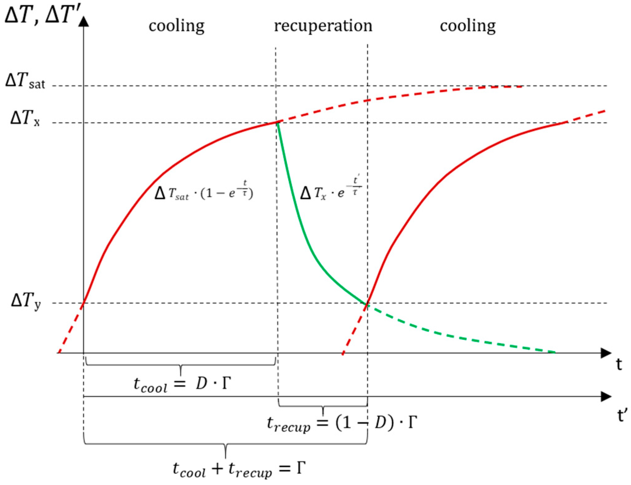
2.1. Theoretical Analysis

The recuperative approach suggested by the authors intends to use the temperature difference created by the Peltier effect (Equation (1)) during the cooling process to recover some part of the supplied electrical energy by employing the Seebeck effect (Equation (2)). In its simplest mathematical form, the Peltier effect creates a heat flow (${\dot{Q}}_P$) proportional to the electric current ($I$) and the Peltier coefficient ($\Pi$). The Seebeck effect generates a voltage ($∆U_S$) proportional to the temperature difference across the thermoelectric element ($∆T$) and the Seebeck coefficient ($S$). According to the second Thomson relation, the Peltier coefficient is equal to the product of the average temperature of the thermoelectric element ($T$) and the Seebeck coefficient. Therefore, Equation (1) can be expressed using the Seebeck coefficient as well. The thermoelectric element is switched as an electric load and electric source alternately for this purpose. Although this approach is intended to increase efficiency by recovering energy, the recovery process itself creates heat flow that may lead to an overall decrease in performance. The electric current generated by the thermoelectric element during recuperation flows in the opposite direction compared to the current supplied during cooling. This reverse current induces a reversed Peltier effect, and hence the opposite heat flow compared to cooling, which reduces useful work. To evaluate benefits and drawbacks and understand the possible applications of the recuperative approach, the interconnected physical processes will be described mathematically.

$${\dot{Q}}_P=\Pi ·I=T·S·I$$

(1)

$$∆U_S=-S·∆T$$

(2)

This study is based on describing thermal processes in a thermoelectric element using the thermal–electrical analogy method. The thermal–electrical analogy method is a mathematical and conceptual approach used in engineering to analyze and solve problems of heat transfer. Being able to describe transient processes with electrical circuits allows for the application of well-established principles and techniques from electrical circuit theory. Circuits can be transformed and simplified to analyze the transient processes of heat transfer. As a result, it is possible to obtain several equations to describe the recuperative approach for a thermoelectric element and predict its influence on thermal and electric processes.

It is preferable to create the model for the thermal–electrical analogy to be as basic as possible in order to achieve relative simplicity of equations and better understand the relation between separate variables. For this purpose, the model of the thermoelectric element (Figure 1) will consist of two capacitors ($C$) that describe the thermal mass on each side of the thermoelectric element, a resistor ($\theta$) between these two capacitors that describes the heat conduction path between the sides of thermoelectric element responsible for heat backflow (${\dot{Q}}_B$), and a current source that represents the heat transfer according to the Peltier effect (${\dot{Q}}_P$). The task for the thermoelectric cooler is to transfer heat from one side (cold side) to the other side (hot side) of the thermoelectric element. The transfer of the heat will be observed as the temperature difference between both sides of the thermoelectric element ($∆T$). The model will describe a thermally isolated thermoelectric element with no heat load or dissipator. Although Joule heating is a very significant factor for real cooling systems, it can be ignored, as it should not directly influence the temperature difference between the hot and cold sides of the thermoelectric element but will contribute to the heat amount on both sides equally. The Seebeck effect will be represented as a voltage source that depends on the temperature difference ($U_S\left(∆T\right)$). This voltage source is connected in series with the electrical resistance of the thermoelectric element ($R_i$) and a resistor that represents the external electrical load ($R_L$). The Thomson effect and other thermoelectric effects will be ignored for the simplicity of the model.

The thermal–electrical analogy model shown in Figure 1 can be simplified by applying principles of electrical circuit theory in order to use basic mathematical expressions of RC circuits to describe the transient heat response of a thermoelectric element. A current source with parallel resistance can be converted to a voltage source with series resistance, as shown in Figure 2a. If the current source represents a heat flow, the voltage source represents a temperature difference. The heat flow due to the Peltier effect (${\dot{Q}}_P$) presented in Figure 1a moves heat from the cold side to the hot side of the thermoelectric element, increasing the temperature difference across the resistance $\theta$ and thus the heat backflow (${\dot{Q}}_B$). At a certain point, both heat flows become equal, and the temperature difference reaches saturation. This saturation temperature difference ($∆T_{sat}$) is the output value of the voltage source and can be calculated according to Equation (4). The ground connection usually represents the ambient temperature; however, this model is aimed at analyzing temperature differences rather than absolute temperature values. Moreover, the thermoelectric element will be considered thermally isolated. Therefore, capacitors can be relocated and put directly in series (Figure 2b), hence considered as a single capacitor (Figure 2c). The total heat flow through this circuit (${\dot{Q}}_{\mathsf{\Sigma }}$) is the difference between ${\dot{Q}}_P$ and ${\dot{Q}}_B$. It is equal to zero once $∆T$ reaches the $∆T_{sat}$ value.

The circuit in Figure 2c is reduced to a basic RC circuit with a voltage source. All the transient processes of heat flow to the thermal mass of the thermoelectric element can be described as charging a capacitor through a resistor with a constant voltage source. For example, the temperature difference will change according to the following curve during the cooling process:

$$∆T\left(t\right)=∆T_{sat}·{(1-e}^{-\frac{t}{\tau }})$$

(3)

The value $\tau$ is the time constant for the temperature difference change and can be calculated by multiplying the thermal resistance $\theta$ and the thermal capacitance $C^{\prime }$. The temperature difference will reach a value that is very close to $∆T_{sat}$ after a time equal to 5$\tau$; $∆T_{sat}$ can be calculated by Equation (4) and merged with Equation (1):

$$∆T_{sat}={\dot{Q}}_P·\theta =T·S·I·\theta$$

(4)

The thermoelectric element will reach a certain temperature difference ($∆T_x$) if cooling is performed for a limited time. The temperature difference will decrease according to Equation (5), starting from $∆T_x$. The temperature difference and time values specific to recuperation will include an apostrophe.

$$∆T\prime \left(t\prime \right)=∆T_x·e^{-\frac{t\prime }{{\tau }^{\prime }}}$$

(5)

It is important to emphasize that the time constant in Equation (2) is written with an apostrophe. It is necessary because of the additional Peltier effect heat flow created by the electric current generated during recuperation, which is opposite to the current flow during cooling. The additional heat flow will contribute to the naturally observed heat backflow due to thermal conduction through $\theta$. This results in a faster $∆T^{\prime }$ decrease and therefore a decrease in the $\tau \prime$ value. The time constant during recuperation ${\tau }^{\prime }$ can be equal to the time constant during cooling $\tau$ if no electrical load is connected to the thermoelectric element during recuperation.

Equations (3) and (5) describe a non-periodic case of recuperation where cooling is performed for a limited amount of time and is succeeded by infinite recuperation. This might be applied in a case where recuperation is long enough for $∆T$ to become equal to 0; however, shorter recuperation times are more probable. If cooling is restarted before $∆T$ has reached 0, this temperature difference will be the starting point of the new cooling cycle. The temperature difference at the end of recuperation $∆T_y$ will contribute to $∆T_x$, which can be reached during the limited time of cooling. The change in the temperature difference during periodic recuperation is shown in Figure 3.

Figure 3 illustrates the curves of the temperature difference expected according to Equations (3) and (5), which are continued by dashed lines; however, due to the interruption of the cooling and recuperation process, the temperature difference is forced to follow the solid line. The horizontal axis represents the possible cooling time ($t_{cool}$) and recuperation time ($t_{recup}$), additionally expressed using duty cycle $D$ and the mode switching period $\mathrm{\Gamma }$.

$$∆T(t)=∆T_{sat}·\left(1-e^{-\frac{t }{\tau }}\right)+∆T_y·e^{-\frac{t}{\tau }}$$

(6)

where temperatures $∆T_y$ and $∆T_x$ are calculated as follows:

$$∆T_y=∆T_x·e^{-\frac{t_{recup}}{{\tau }^{\prime }}}$$

(7)

$$∆T_x=∆T_{sat}·\frac{1-e^{-\frac{t_{cool}}{\tau }}}{1-e^{-\left(\frac{t_{cool}}{\tau }+\frac{t_{recup}}{{\tau }^{\prime }}\right)}}$$

(8)

All the acquired equations, in conjunction with thermoelectric effect relations and basic laws of physics, can be used to find equations that describe the relations for estimating the impact of recuperation. For easier readability of the following equations, a set of parameters that describe the performance of the thermoelectric element is introduced, as these parameters are present in most of them. This parameter set is called the thermoelectric element figure of merit $ZT$ and can be calculated by following equation:

$$ZT=\frac{T·S^2·\theta }{R_i}$$

(9)

Gains from the recuperation approach can be estimated as the ratio between recuperated and supplied electric energy:

$$\frac{E_{recup}}{E_{supply}}=\frac{1}{2}·Z{T}^2·\frac{R_i·R_L}{{{(R}_i+R_L)}^2} · \frac{{\tau }^{\prime }}{t_{cool}}· \frac{ \left(1-e^{-\frac{2·t_{recup}}{{\tau }^{\prime }}}\right)·{\left(1-e^{-\frac{t_{cool}}{\tau }}\right)}^2}{1-e^{-\left(\frac{t_{cool}}{\tau }+\frac{t_{recup}}{{\tau }^{\prime }}\right)}}$$

(10)

Equation (10) can be split into three parts regarding the nature of dependance:

• Thermoelectric element figure of merit $ZT$;
• Electrical resistance of the thermoelectric element $R_i$ and electrical load resistance $R_L$;
• Time spent in cooling $t_{cool}$ and recuperation modes $t_{recup}$ relative to the thermal time constant.

It is important to notice that this ratio does not depend on the amount of supplied current, and theoretically, it should be possible to recover the same relative amount of energy regardless of the cooling power. In practice, it might lead to a change in cooling efficiency because of a change in average temperature, which will lead to a change in the $ZT$ value.

The $ZT$ value is a set of properties that describe the thermoelectric element. The highest possible value is always desirable; however, it is usually limited by the cost of thermoelectric elements and the availability of ever-advancing technologies. The significance of the $ZT$ value is further amplified by being squared in the equation. The relative recuperated energy amount depends on the ratio between $R_i$ and $R_L$ values, and thus absolute values are not significant from this perspective. The amount of relative recuperated energy depends greatly on cooling and recuperation time. Moreover, the time-dependent part of Equation (10) consists of two time constants $\tau$ and ${\tau }^{\prime }$, which might be different, and this difference might be influenced by both $ZT$ and the ratio between $R_i$ and $R_L$ due to the reasons discussed in following analysis.

Recovering electrical energy is a favorable property of the recuperation approach; however, the current flow generated by the thermoelectric element during recuperation creates a Peltier effect-induced heat flow that flows in the opposite direction compared to the heat flow during cooling. Additional heat backflow that is created by recuperation leads to a loss of overall efficiency of cooling performance. Such an undesirable impact could be described as the ratio between the decrease in the average heat amount that can be transported due to recuperation ($Q_{loss}$) and the average transported heat without it ($Q_{avg}$). As the average transported heat $Q_{avg}$ is proportional to the average temperature difference $\overline{∆T}$, such relative performance loss can be conveniently calculated by using the mathematically estimated or measured change in average temperature difference. The ratio can be calculated using the following equation:

$$\frac{Q_{loss}}{Q_{avg}}=\frac{Q_{avg}-Q_{avg}^{\prime }}{Q_{avg}}=\frac{\overline{∆T}-\overline{∆T^{\prime }}}{\overline{∆T}}=\frac{\left(\tau -\tau \prime \right)}{t_{cool}}·\frac{\left(1-e^{-\frac{t_{cool}}{\tau }}\right)·\left(1-e^{-\frac{t_{recup}}{{\tau }^{\prime }}}\right)}{1-e^{-\left(\frac{t_{cool}}{\tau }+\frac{t_{recup}}{{\tau }^{\prime }}\right)}}$$

(11)

In contrast from Equation (10), Equation (11) depends only on the relative time spent in cooling and recuperation modes and does not include direct dependence on the thermoelectric element figure of merit $ZT$ or the value of load resistance $R_L$. However, these factors indirectly influence the ratio through the change in the time constant ${\tau }^{\prime }$. The ratio between the time constants for cooling and recuperation (${\rm Y}$) can be calculated by Equation (11), and it depends only on $ZT$ and the relative $R_L$ value.

$${\rm Y}=\frac{\tau }{{\tau }^{\prime }}=ZT·\frac{R_i}{R_i+R_L}+1$$

(12)

Equation (12) allows for the evaluation of the impact of the recuperation approach by using only the time constant for the cooling mode $\tau$, which should be constant and can be measured regardless of the recuperation tactics.

Equations (10) and (11) allow for the theoretical estimation of relative gains and losses that are created by implementing the suggested recuperation approach for thermoelectric cooling. The ratio between these two quantities will show how rational such an implementation is. This quantity will be called the “Figure of recuperation implementation rationality” $\Psi$. It can be calculated by Equation (13).

$$\Psi =\frac{\frac{E_{recup}}{E_{supply}}}{\frac{Q_{loss}}{Q_{avg}}}=\frac{1}{2}·ZT· \frac{R_L}{R_i+R_L} ·\left(1+e^{-\frac{t_{recup}}{{\tau }^{\prime }}}\right)·\left(1-e^{-\frac{t_{cool}}{\tau }}\right)$$

(13)

If the $\Psi$ value is lower than 1, then the losses induced by the recuperation are greater than the benefits. In this case, periodic recuperation is irrational.

Such an analysis allows for the prediction and understanding of the influence of different variables within this process.

For the analysis of the proposed mathematical relations, Equations (10), (11), and (13) will be examined by performing iterative calculations using different sets of values for separate variables within a practically expected range.

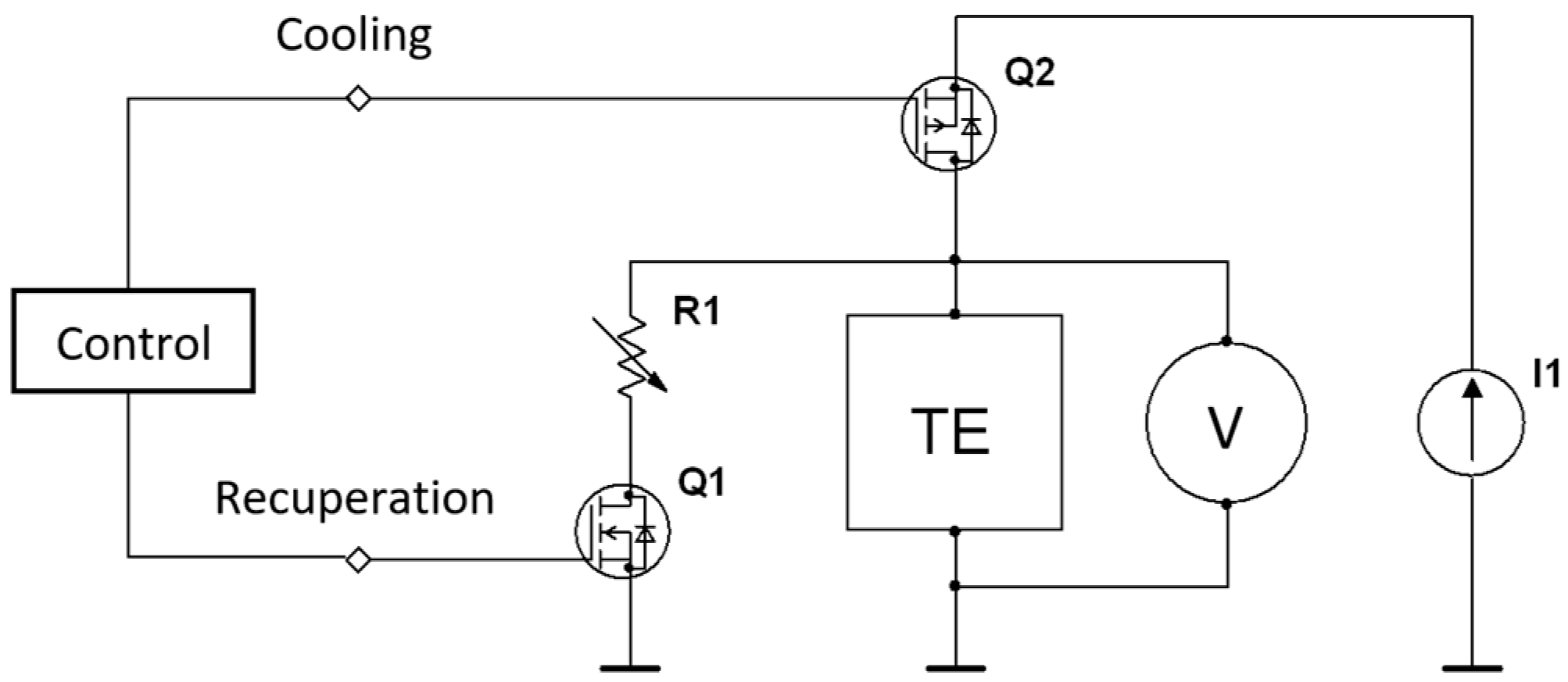
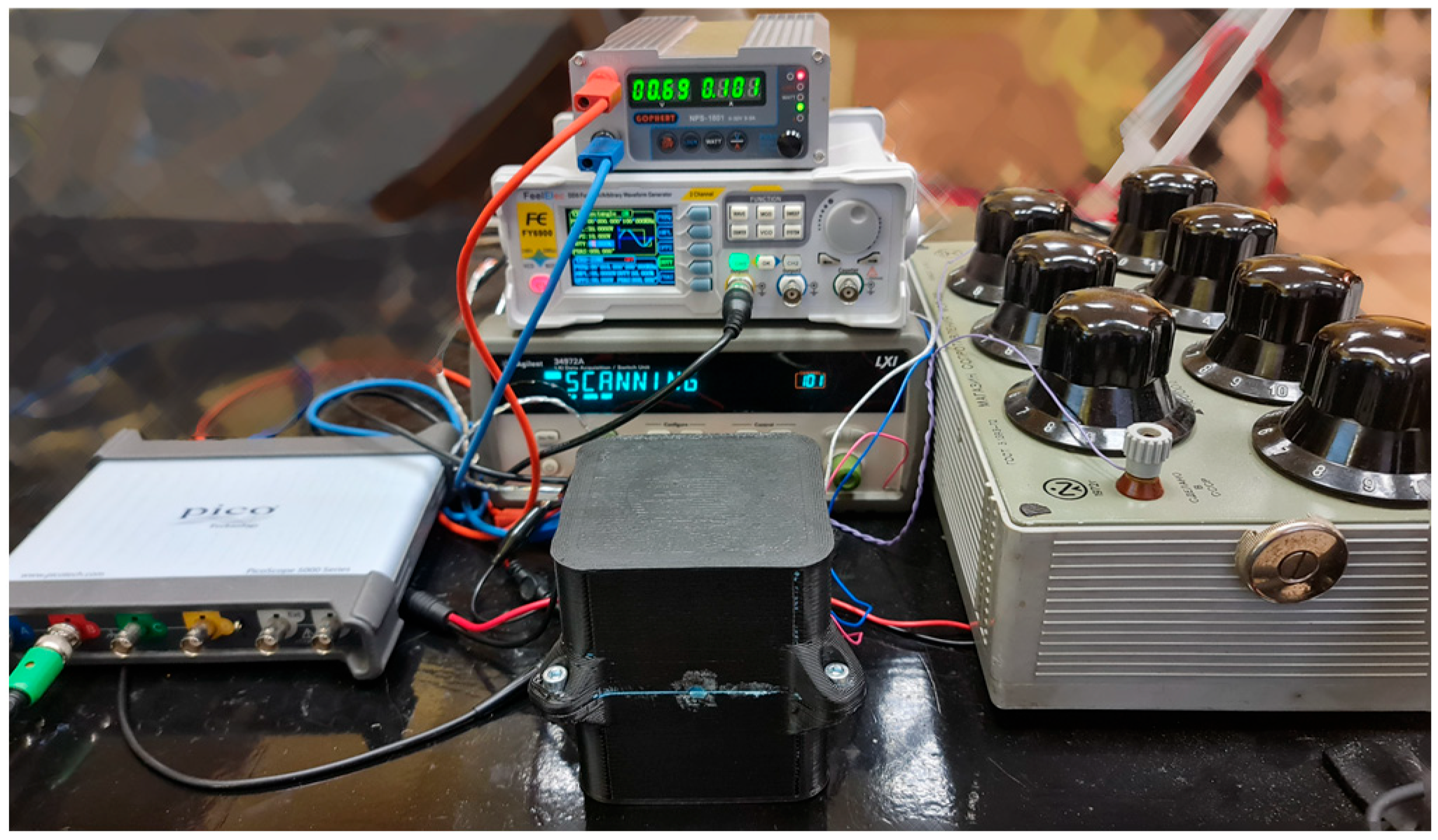
2.2. Experimental Procedure

Analytically, the predicted influence of variables will be verified experimentally using a commercially available thermoelectric element GM250-127-10-15 [29] produced by European Thermodynamics. Electrical power for cooling will be supplied by an adjustable constant current source. Energy generated during recuperation will be dissipated on the ohmic load in the form of a precision resistor decade box. Modes are switched by MOSFET transistors which are controlled by a MOSFET driver and an arbitrary signal generator.

To estimate the amount of supplied and recuperated energy, voltages across the thermoelectric element and mode switching signals are measured by PC oscilloscope PicoScope 5444D (Pico Technology, St Neots, UK). This will allow the estimation of the precise amount of time spent in both modes. Power and energy during the recuperation mode will be estimated by using voltage measurements and the precise value of the resistive load. The supplied electrical power and energy will be calculated using voltage measurements and the current value set for the constant current supply. A simplified electric schematic of the experimental setup is shown Figure 4.

To keep the thermoelectric element thermally isolated from the ambient environment, it is placed in a 3D-printed enclosure that is filled with heat insulation foam, which is cured with a thermoelectric element inside of it. Such an enclosure creates approximately 106 K/W thermal resistance to the ambient environment. Temperatures are measured by an Agilent 34872A data logger (Keysight, Santa Rosa, CA, USA) with 10 kΩ NTC thermistors that are placed on the hot and cold sides of the thermoelectric element and several thermistors inside and outside the enclosure. The experimental setup can be seen in Figure 5. Calculating the temperature difference between the hot and cold side of the thermoelectric element with and without the recuperation load and using Equation (11) will allow the estimation of heat loss induced by recuperation. Equation (11) allows the use of average temperature difference values. This requirement greatly simplifies the temperature measurement procedure, as the thermal inertia of the thermoelectric element as well as the response time of the temperature sensors do not impact the average temperature values experienced by the temperature sensors. Nevertheless, it is important to consider the timestep of temperature measurements when choosing the time spent in one mode switching period $\mathrm{\Gamma }$ to minimize the effects of aliasing when averaging.

The current research studies the influence of cooling and recuperation time as well as the influence of load resistance for the recuperation mode on the cooling performance of the thermoelectric element. The influence of the $ZT$ value was not estimated, as it is impossible to reliably alter this parameter without affecting other variables. The experimentally estimated $ZT$ value for the thermoelectric element used for the experiment is 0.64.

The estimated value of $\tau$ for the $∆T$ change of this setup was 33.22 s. The measurements for both the temperature difference and electrical energies were conducted in sets of certain cooling and recuperation times, which were expressed in the form of duty cycle $D$ and relative time period $\frac{\Gamma }{\tau }$ for the more convenient adjustment of equipment settings. Experimental data were acquired at the following values of $D$ = 0.05, 0.1, 0.25, 0.5, 0.75, 0.9, 0.95 and $\frac{\Gamma }{\tau }$ = 0.06, 0.12, 0.241, 0.482, 0.753, 0.994, 1.988, 3.012. Such specific $\frac{\Gamma }{\tau }$ values were chosen as the measure of anti-aliasing for periodic temperature measurements. The range of the duty cycle was limited by a necessity to maintain comparable cooling power throughout all of the duty cycle values, as a very high peak current would be necessary at low duty cycle values to keep the performance reasonable and thus $∆T$ values high enough at higher duty cycle values. Each of the 56 combinations of $D$ and $\frac{\Gamma }{\tau }$ were measured both with a matched resistive load and without the load for recuperation, resulting in 112 sets of data. A theoretical analysis for the same relations was performed by iterative calculations and presented in the range of 5$\tau$ for cooling and recuperation time. Data are presented as 2D contour plots with duty cycle $D$ and relative time period $\frac{\Gamma }{\tau }$ as one type and relative cooling time $\frac{t_{cool}}{\tau }$ and relative recuperation time $\frac{t_{recup}}{\tau }$ as the other type of argument for time dependance. The representation of the experimental results with regard to cooling and recuperation time is limited, as the sum of these time values cannot exceed the highest value of $\frac{\Gamma }{\tau }$. Therefore, the contour plot has a triangular shape.

Additional measurements were made to study the same three equations at different recuperation load resistances. Measurements were performed at the following values of relative recuperation load: $\frac{R_L}{R_i}$ = 0.01, 0.5, 1, 2, 3, 5, 50, 10,000. Other parameters were held constant: $D$ = 0.8, $\frac{\Gamma }{\tau }$ = 0.3, $I$ = 100 mA. These parameters are not optimal for the best performance; however, they enabled consistent results with the rapid change of variables.

3. Results

The current section presents mathematically obtained data as 2D contour plots to analyze the predicted influence of time parameters in Equations (10), (11), and (13). To validate the theoretical predictions, experiments that can present the equivalent influence of time parameters are conducted, and the results are presented in a similar manner. Theoretical and experimental data are compared.

3.1. Analytical Predictions for Time Dependance of Recuperation

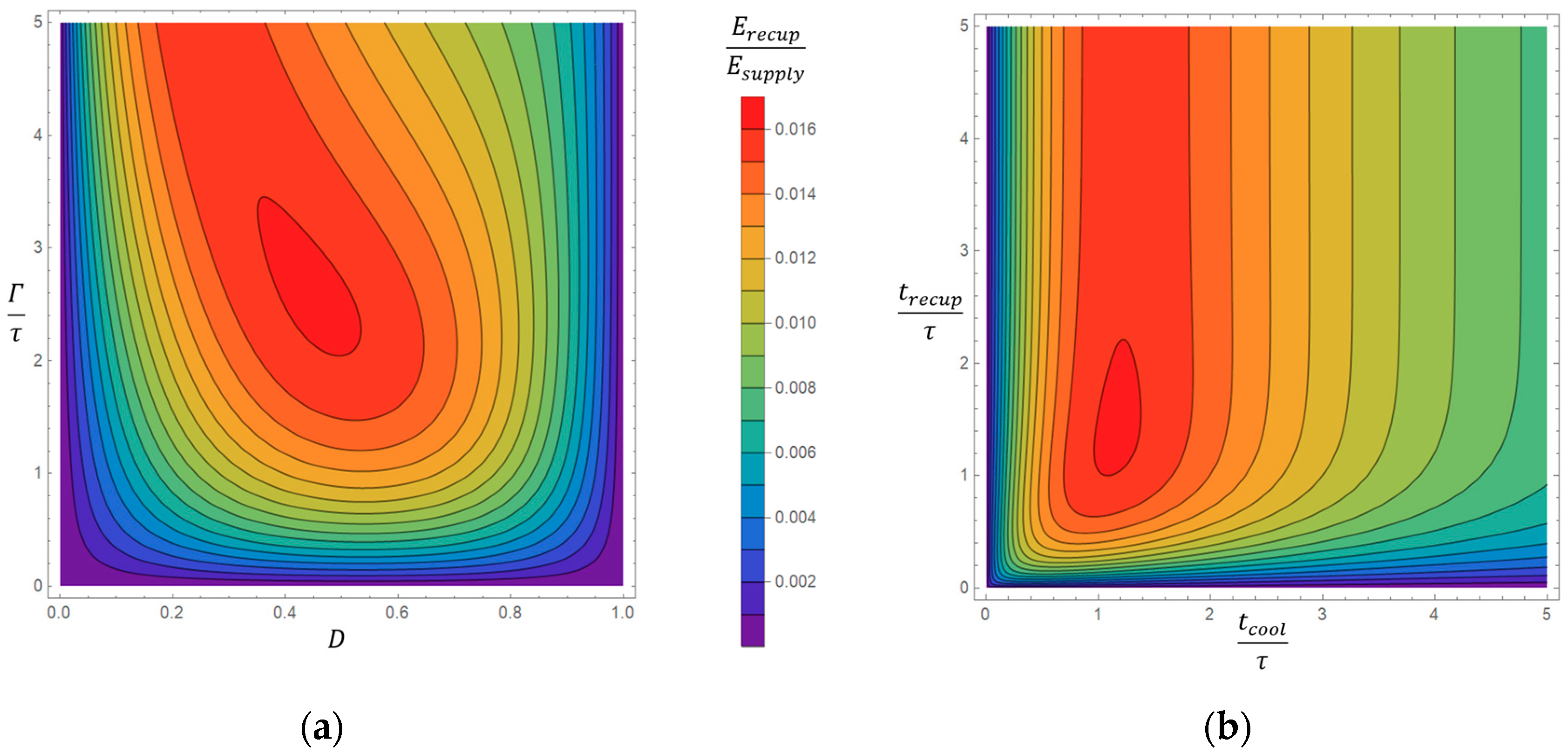
3.1.1. Relative Amount of Recuperated Electrical Energy

Figure 6 shows that the amount of relative recuperated energy is strongly dependent on cooling and recuperation time. As can be seen in Figure 6b, the function shows a clear maximum at values $t_{cool}$ = $t_{recup}$ = 1.25$\tau$. The relative amount of recuperated energy sharply decreases once cooling and recuperation times become lower than 1$\tau$. The recuperation time does not impact the result much at values above 1.25$\tau$; however, it gradually decreases with the increase in cooling time above 1.25$\tau$. In Figure 6a, we can observe that the highest amount of recuperated energy is observed at $D$ = 0.5 and $\frac{\Gamma }{\tau }$ = 2.5$\tau$. Outside these values, the amount decreases gradually, with a slight decrease in the best duty cycle value with an increase in the relative time period. It is estimated that it is possible to recuperate up to 1.7% of the supplied electrical energy for cooling.

3.1.2. Relative Amount of Additional Heat Losses Due to Recuperation Process

In contrast to the relative amount of recuperated energy, the equation for the relative amount of additional heat losses due to the recuperation process does not have a local maximum. As can be seen in Figure 7a, —at low relative time periods, heat losses are almost inversely proportional to the duty cycle. As the period value increases, this relation is skewed towards low duty cycle values. The highest additional heat losses occur at low duty cycle values. Figure 7b reveals the same dependance; however, it is interesting that at recuperation times above 1$\tau$, heat losses depend mostly on cooling time, as the contour lines become close to vertical. At these settings, approximately 24% of the transported heat is lost due to recuperation.

At cooling and recuperation time settings that yield the highest relative recuperated energy, the recuperation process creates approximately 12% of the additional relative heat losses. This means that by using tactics of the highest energy yield, the gains of recuperation are approximately 7 times lower than the losses.

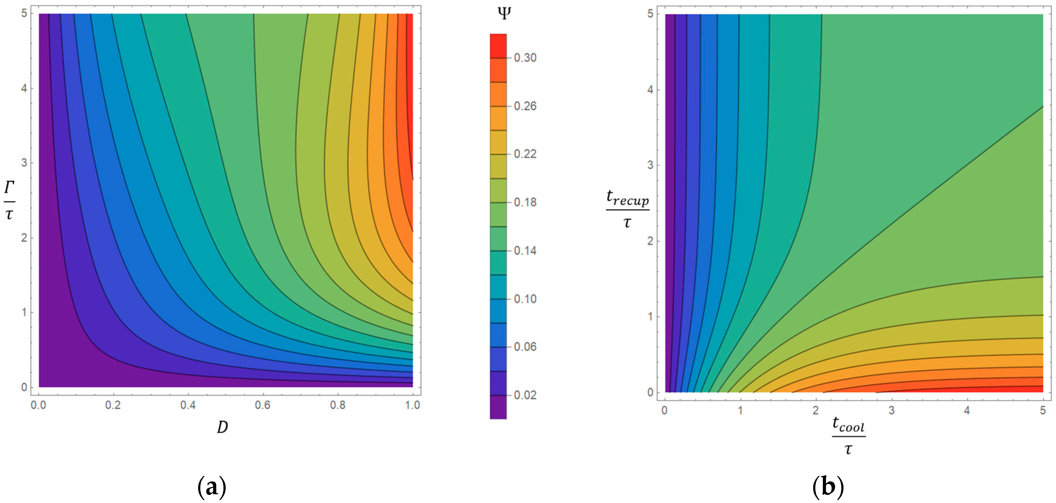
3.1.3. Figure of Recuperation Implementation Rationality

To predict the settings for a more effective recuperation process, it is necessary to calculate the figure of recuperation implementation rationality by Equation (13). The results for these calculations are presented in Figure 8.

According to Figure 8, the highest recuperated energy amounts relative to the induced losses can be achieved when recuperation is conducted rarely and for a short time. The calculations predict the best results if the recuperation time is shorter than 0.25$\tau$ with cooling times higher than 2$\tau$. The highest predicted value of $\Psi$ at a matched recuperation load impedance is 0.31.

3.2. Experimental Results for Time Dependance of Recuperation

The following experimental results present the attempt to validate previous predictions for the impact of cooling and recuperation time duration.

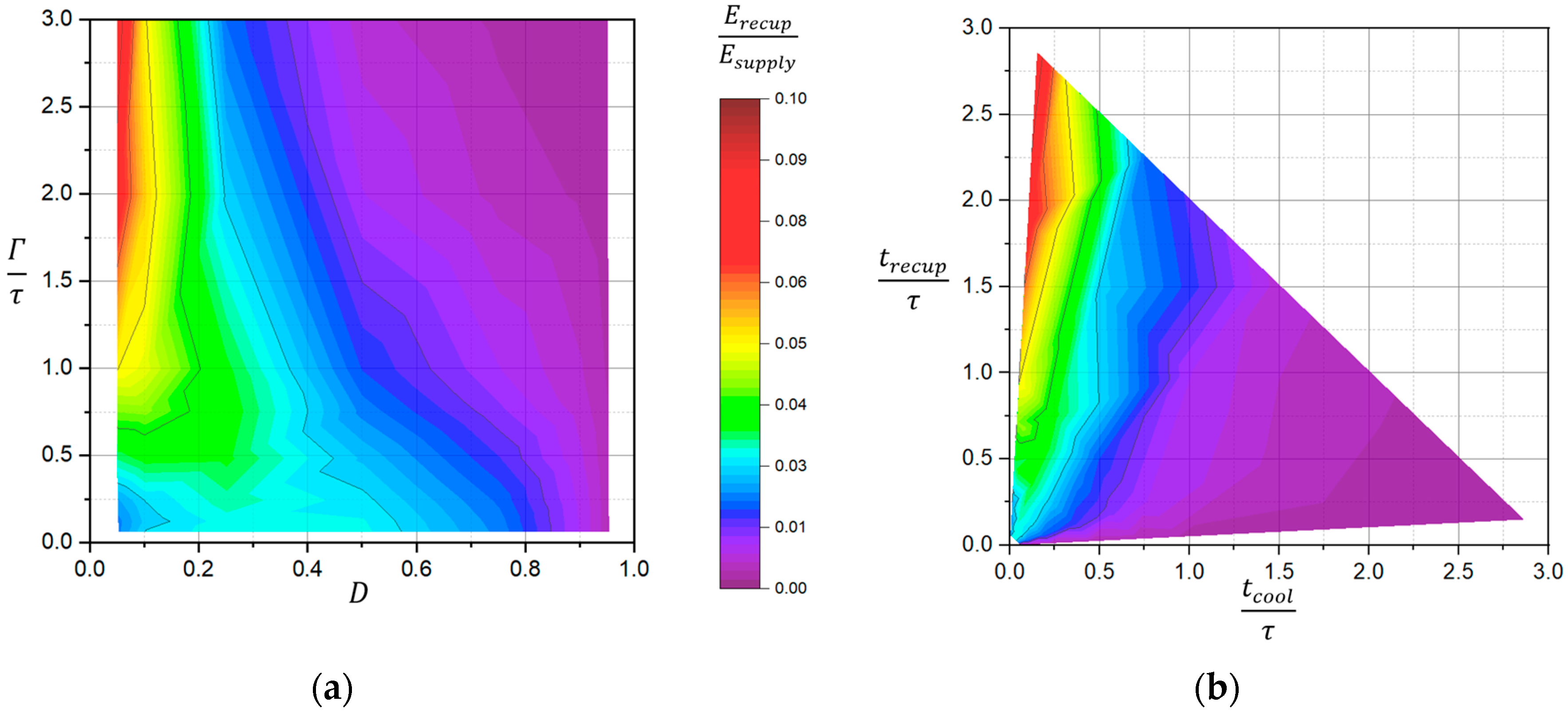
3.2.1. Relative Amount of Recuperated Electrical Energy

The highest amount of relative recuperated energy is reached when the recuperation time is longer than 1.5$\tau$ and the cooling time is shorter than 0.25$\tau$. The highest observed value in this experiment is approximately 10%; however, according to predictions, it should have been approximately 1.7%, thus 5.9 times lower. The results shown in Figure 9 do not reach an obvious local maximum at cooling and recuperation times at 1.25$\tau$ as predicted. Figure 9a shows a slight extension in the range of $D$ = 0.2 and $\frac{\Gamma }{\tau }$ between 0.5 and 1, which might be similar to the curve shown in Figure 6a. Therefore, it is possible that all the values are shifted towards a shorter cooling time compared to the predictions.

3.2.2. Relative Amount of Additional Heat Losses Due to Recuperation Process

The results in Figure 10 show that the relative amount of additional heat losses due to the recuperation process observed experimentally follow a dependance close to the predicted one. The highest relative losses are observed at the shortest cooling times according to Figure 10b, and contour lines become close to vertical at recuperation times longer than 0.5$\tau$. In Figure 10a, we can see similar curves to the predicted ones shown in Figure 7a. The skew of the vertical contour lines of the experimental results is more pronounced, and with an increase in the relative time period, it has more impact on heat losses compared to predictions. The relative heat losses decrease with an increase in the duty cycle. At $D$ = 0.95, recuperation creates about 1–2% of additional losses; however, at $D$ = 0.05, relative heat losses increase to 15–16%. The model predicted about 24% losses at a 0.05 duty cycle.

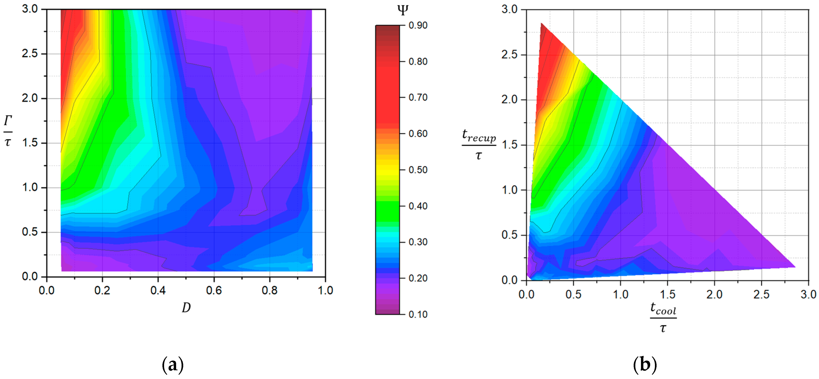
3.2.3. Figure of Recuperation Implementation Rationality

According to Figure 11a, the highest figure of recuperation implementation rationality is achieved at relative time period values above 2$\tau$ and duty cycles smaller than 0.1. In terms of time duration in cooling and recuperation mode, Figure 11b shows the best results at a cooling time shorter than 0.5$\tau$ and a recuperation time longer than 2$\tau$. As shown in Figure 8, the highest $\Psi$ values are predicted at long cooling times and short recuperation times. Experimentally, values as high as 0.9 were reached; however, according to the model, $\Psi$ should not exceed 0.31 with $ZT$ = 0.64.

3.3. Impact of Recuperation Load Resistance

As the results can be shown on a 2D plot, the experimental results will be presented together with the predictions for ease of comparison.

3.3.1. Relative Amount of Recuperated Electrical Energy

Figure 12 shows that the experimental curve mostly follows the predicted shape. There is a difference in the absolute values, and the experimental results are higher than expected. This difference was already observed in previous experiments when comparing Figure 6 and Figure 9. Although the highest value is measured with a matched load, we can assume that the peak value might slightly shift towards higher resistance, as the curve is not symmetric. This would correspond to the predictions that have the maximum offset in the direction of higher resistances as well. The predicted maximum is 0.4%, and the experimental maximum is 1.3%. The experimental values do not contradict the results presented in Figure 9.

3.3.2. Relative Amount of Additional Heat Losses Due to Recuperation Process

The lines shown in Figure 13 are quite close to each other both in shape and values. A heat loss of 5.8% was observed experimentally at the matched load. A loss of 6.0% was predicted by the model. Although the shape of the experimental results seems quite distorted closer to the ends of the vertical scale, it might be the result of the absence of data at loads in the range around 0.1 and 10, as more measurements were performed closer to the matched load. The result at the matched load does not conflict with the previous experimental results shown in Figure 10.

3.3.3. Figure of Recuperation Implementation Rationality

As can be seen in Figure 14, it is theoretically predicted that the $\Psi$ value should increase with an increase in resistance and tend to plateau as the load resistance becomes 10 times higher than the internal resistance of the thermoelectric element. However, experimentally, we observe a peak at a load that is 3 times higher than the internal resistance of the element with a value of 0.27. The value at the matched load is 0.22, which corresponds to the experimental results presented in Figure 11.

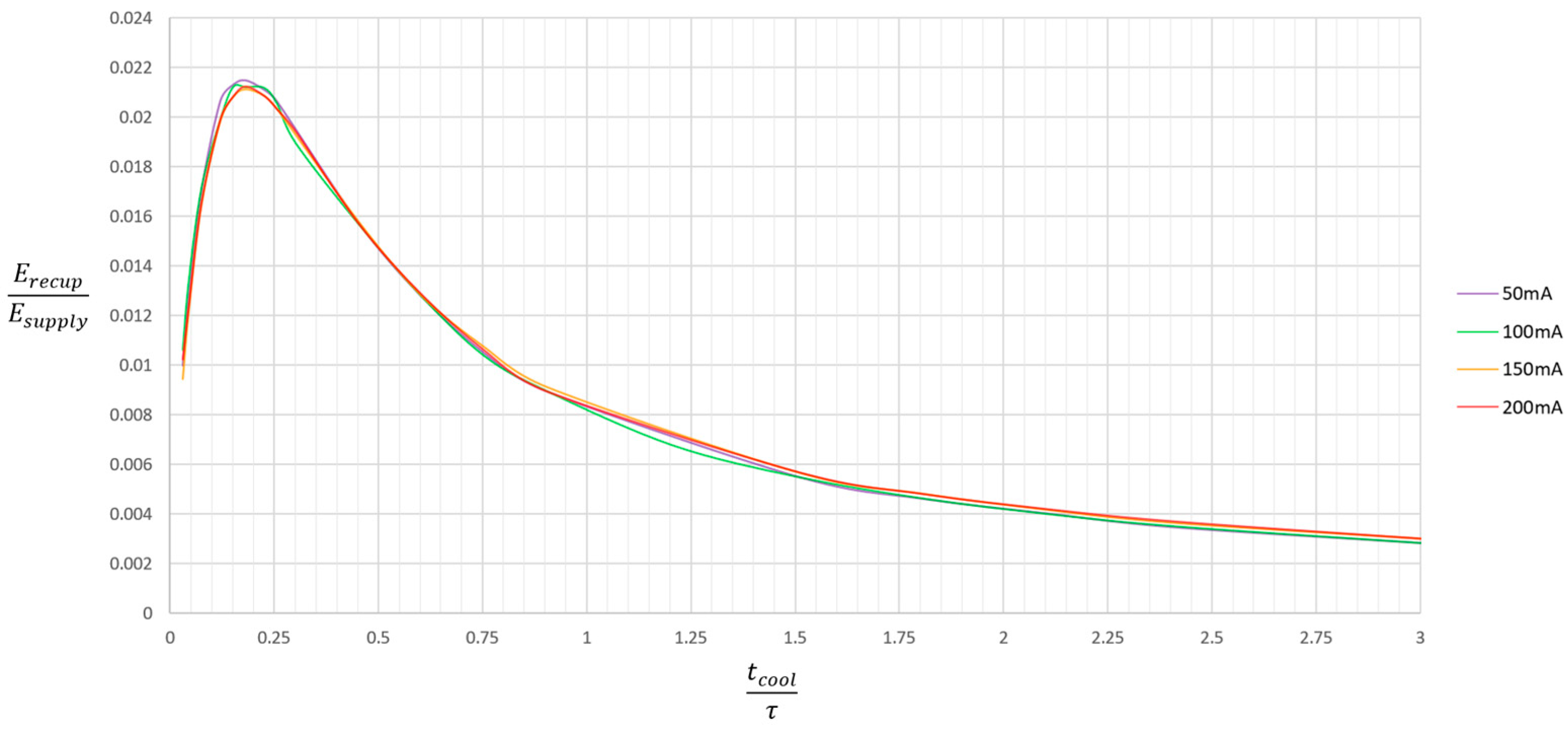
3.4. Additional Measurements of Relative Amount of Recuperated Electrical Energy at Short Cooling Times

In order to observe the relative amount of recuperated electrical energy at shorter cooling times, an additional experiment was performed with the same experimental setup, as the experimental results in Section 3.2.1 did not present an obvious local maximum. In this experiment, the recuperation process can be assumed to be non-periodic as, after a certain cooling duration, the thermoelectric element was switched to recuperation mode until the setup reached a steady state thermally and the temperature difference became very close to zero. The value of $t_{recup}$ exceeds the value of 5$\tau$. The cooling time was set in the range from 0.03$\tau$ to 3$\tau$. Four different current values were supplied to the thermoelectric element during cooling: 50 mA, 100 mA, 150 mA, and 200 mA. The average cooling power was not kept constant due to the non-periodic cooling and permissible precision for temperature measurements. Recuperation was performed with a matched resistive load. The experimental results are presented in Figure 15.

The predicted local maximum of the function was observed experimentally. The peak is shifted to shorter cooling time durations, as assumed in Section 3.2.1. The highest relative amount of recuperated electrical energy is achieved at $t_{cool}$ = 0.18$\tau$. This might indicate that the time constant for the electrical part of the thermal–electrical model might be 7 times shorter than the thermal time constant. Unfortunately, it is hard to estimate the exact $\tau$ from the measurements of the generated voltage, as the initial value of the exponential decay curve is influenced by parasitic capacitances and inductances of the oscilloscope, cables, switching circuitry, and thermoelectric element. A rough estimate would suggest a value of approximately 4 s.

It is possible to recuperate approximately 2.1% of the supplied energy at the peak. To compare this result to the analytical estimations, Equation (10) can be simplified due to the assumption of infinite recuperation time. If the newly obtained time constant is used for both $\tau$ and ${\tau }^{\prime }$, a 2.1% result would be achieved at $ZT$ being approximately 0.64.

The use of a different time constant for Equation (10) would alter the predicted curve of the relative amount of recuperated electrical energy shown in Figure 12, moving the predicted values closer to the experimental results.

As can be seen in Equation (10), it does not contain the current as a variable, suggesting that the relative amount of recuperated electrical energy does not depend on the amount of electrical current supplied for cooling purposes. This prediction is validated by the results of this experiment, as all four lines obtained at different current values match each other with a minor deviation.

4. Discussion

4.1. Time Dependance of Recuperation Process

The results for time dependance are presented in 12 contour plots (Figure 6, Figure 7, Figure 8, Figure 9, Figure 10 and Figure 11). The mathematical model of additional heat loss created by the recuperation approach was successfully validated experimentally. The absolute values between the predictions and experimental results differed slightly, which might be the result of the simplification of the model. In particular, the model treats the thermal mass, thermal resistance, and other parameters as uniform rather than distributed properties, resulting in temperature and heat flow gradients throughout the element. However, such simplification is acceptable for general estimations and could be improved by implementing additional coefficients to compensate for the error. This difference might be also the result of higher amounts of electrical energy being generated during recuperation, thus creating more heat backflow. As measurements were performed with a thermoelectric element that is not completely isolated from the ambient environment, there might be some influence from changes in the ambient environment. According to both the predictions and experimental results, it is advisable to keep the recuperation time as short as possible to decrease the amount of heat loss created by recuperation. Such conditions will also decrease heat loss due to regular backflow.

The experimental results qualitatively validated the suggested analytical model for the relative recuperated amount of electrical energy; however, a dependence was observed at shorter cooling times and longer recuperation times than the model predicted. Additional measurements shown in Figure 15 reveal the local maximum for the relative amount of recuperated energy, showing that the optimal cooling time is observed at $t_{cool}$ = 0.18$\tau$, which is about 7 times lower than predicted. This offset can be explained by the spatially distributed nature of the thermoelectric element’s properties, which were not fully accounted for in the heavily simplified thermal–electrical analogy model, compromising the precision of its predictions. The difference in the predicted and measured $\Psi$ values is the result of the time constant offset for the relative amount of recuperated energy predictions. The thermal–electrical analogy model needs to take into account the difference in the transient response of electric and thermal processes within the thermoelectric element. The results for additional measurements of the relative recuperated amount of electrical energy at shorter cooling times suggest that more precise results might be achieved with minor adjustments in Equation (10) in order to maintain the simplicity of the analytical models developed in future studies. The minimalism of the model allows for convenient estimation without involving SPICE or CAD software.

In most use cases, recuperation will not be a primary task of the cooling system; therefore, it has to be implemented in a way that does not counteract the primary function of the system. It is impossible to outweigh the losses by benefits when using thermoelectrical elements that do not have high $ZT$ values. Losses due to the transformation, transmission, and storage of recuperated energy will contribute to the overall loss of efficiency due to the recuperation. The highest $\Psi$ values are achievable when operating the thermoelectric element with short cooling times and long recuperation times. This means that this solution might be more reasonable for systems with occasional cooling demands and periodic idling. This approach might be applied in cases of target temperature overshoot, which forces the temporary termination of cooling. The recuperative approach might be viable in cases when the termination of cooling is necessary or inevitable, for example, during thermal shutdown or a power outage, as the temperature difference between the hot and cold sides of the thermoelectric element will come to equilibrium with or without applying the recuperation. An additional amount of energy in an unfortunate event might be advantageous for less power-demanding tasks, such as temperature monitoring, information storage, or safe shutdown of the system.

4.2. Impact of Recuperation Load Resistance

The relative amount of additional heat loss at the different recuperation load resistances observed experimentally matched the predictions of the proposed model. In the used setup, approximately 6% of the transported heat is lost due to recuperation at matched load impedance. At loads that are close to the short circuit, more than 10% of the heat transported by cooling flows back because of recuperation. Such a load might be beneficial in cases when cooling is not necessary; however, some temperature difference is created across the thermoelectric element by an external heat load. In this case, heat flow might be assisted by recuperation, and heat can be transported at a higher rate due to the Peltier effect that is created by the current flow during recuperation. The use of the Seebeck effect to generate heat flow due to the Peltier effect is also known as Variable Thermal Resistance [30,31,32].

The experimental results for the relative amount of recuperated electrical energy qualitatively matched the predicted curve; however, a difference in absolute values was observed. This difference is most likely caused by the shorter time constant for thermal processes during the thermoelectric generation mode. It was observed that a higher relative amount of energy might be recuperated with resistances slightly above the matched load impedance value. The decrease in electrical load should lead to a reduction in additional heat losses as well.

The experimentally estimated figure of recuperation implementation rationality showed that an increase in resistance for the recuperation load might be beneficial, as a peak is observed at a load that is 3 times higher than the internal resistance of the thermoelectric element. Although it might be more efficient theoretically, the practically achievable amount of recuperated electrical energy has to be taken into account, as voltage conversion and energy storage might become more difficult and less efficient at low voltage levels. A decrease in $\Psi$ values was observed at higher load resistances, contrary to the predicted level settling close to a constant value. This might be explained by higher heat losses at these load values without a proportional generation of energy.

5. Conclusions

An analytical model based on the thermal–electrical analogy method to estimate the impact of the proposed recuperation approach on the performance of the thermoelectric element was developed and experimentally validated. Three quantities for evaluating the impact of the recuperation approach were suggested in the form of mathematical equations. The method for the experimental estimation of these quantities was presented. All three quantities depend on the set of thermoelectric element properties combined: the thermoelectric element figure of merit $ZT$, the ratio between the equivalent series resistance of thermoelectric element $R_i$ and the electrical load for the thermoelectric element during the recuperation $R_L$, and the time spent in cooling and recuperation modes—$t_{cool}$ and $t_{recup}$.

The proposed model simplifies complicated thermal processes, allowing prediction of the viability of electrical energy recuperation during cooling without the need for complex computer simulations.

The quantity for estimating possible benefits, called the relative amount of recuperated electrical energy, is the ratio between recuperated electrical energy and electrical energy supplied for cooling purposes. The experimental results confirmed the curve predicted by the equation; however, the precision of the thermal–electrical analogy model is decreased due to the profound reduction of its complexity.

The relative amount of additional heat loss due to the recuperation process is the quantity that estimates the drawbacks of recuperation implementation due to additional heat flow created by the recuperation process. The predictions were validated experimentally with acceptable precision.

The ratio between two previously described quantities is called the figure of recuperation implementation rationality, and it compares the benefits and drawbacks of the recuperation approach, thus pointing out whether it is a rational solution. The experimental results confirm the predictions only partially due to the insufficient accuracy of the analytical estimation for the relative amount of recuperated electrical energy.

It was concluded that recuperation might be beneficial in cases when the interruption of the cooling process is necessary or inevitable, as the amount of recuperated energy could outweigh the induced losses only by the use of thermoelectric elements with high $ZT$ values, which are not available at the moment.

The presented methodology for estimating the impact of the recuperative cooling approach could be further improved by including external heat sources and heat sinks into the thermal–electrical analogy model, as well as the impact of Joule heat created by current flow through the thermoelectric element.

References

1. Abdul-Wahab, S.A.; Elkamel, A.; Al-Damkhi, A.M.; Is’ Haq, A.; Al-Rubai’ey, H.S.; Al-Battashi, A.K.; Al-Tamimi, A.R.; Al-Mamari, K.H.; Chutani, M.U. Design and experimental investigation of portable solar thermoelectric refrigerator. Renew. Energy 2009, 34, 30–34. [Google Scholar] [CrossRef]
2. Snyder, G.J.; LeBlanc, S.; Crane, D.; Pangborn, H.; Forest, C.E.; Rattner, A.; Borgsmiller, L.; Priya, S. Distributed and localized cooling with thermoelectrics. Joule 2021, 5, 748–751. [Google Scholar] [CrossRef]
3. Putra, N.; Sukyono, W.; Johansen, D.; Iskandar, F.N. The characterization of a cascade thermoelectric cooler in a cryosurgery device. Cryogenics 2010, 50, 759–764. [Google Scholar] [CrossRef]
4. Chowdhury, I.; Prasher, R.; Lofgreen, K.; Chrysler, G.; Narasimhan, S.; Mahajan, R.; Koester, D.; Alley, R.; Venkatasubramanian, R. On-chip cooling by superlattice-based thin-film thermoelectrics. Nat. Nanotechnol. 2009, 4, 235–238. [Google Scholar] [CrossRef]
5. Baker, A.A.; Thuss, R.; Woollett, N.; Maich, A.; Stavrou, E.; McCall, S.K.; Radousky, H.B. Cold Spray Deposition of Thermoelectric Materials. JOM 2020, 72, 2853–2859. [Google Scholar] [CrossRef]
6. Yang, L.; Chen, Z.-G.; Dargusch, M.S.; Zou, J. High Performance Thermoelectric Materials: Progress and Their Applications. Adv. Energy Mater. 2018, 8, 1701797. [Google Scholar] [CrossRef]
7. Lindler, K.W. Use of multi-stage cascades to improve performance of thermoelectric heat pumps. Energy Convers. Manag. 1998, 39, 1009–1014. [Google Scholar] [CrossRef]
8. Huang, H.-S.; Weng, Y.-C.; Chang, Y.-W.; Chen, S.-L.; Ke, M.-T. Thermoelectric water-cooling device applied to electronic equipment. Int. Commun. Heat Mass Transf. 2010, 37, 140–146. [Google Scholar] [CrossRef]
9. Liu, D.; Cai, Y.; Zhao, F.-Y. Optimal design of thermoelectric cooling system integrated heat pipes for electric devices. Energy 2017, 128, 403–413. [Google Scholar] [CrossRef]
10. Lu, Y.; Cui, J.; Zhao, Y. Ultra-precision temperature control of circulating cooling water based on fuzzy-PID algorithm. In Proceedings of the Tenth International Symposium on Precision Engineering Measurements and Instrumentation, Kunming, China, 8–10 August 2018; p. 1105348. [Google Scholar] [CrossRef]
11. Koç, T.; Bayhan, N. Control of a Thermoelectric Cooling Module by Metaheuristic Optimization Algorithms. J. Aeronaut. Space Technol. 2024, 17, 89–106. [Google Scholar]
12. Harvey, R.D.; Walker, D.G.; Frampton, K.D. Enhancing Performance of Thermoelectric Coolers through the Application of Distributed Control. IEEE Trans. Compon. Packag. Technol. 2007, 30, 330–336. [Google Scholar] [CrossRef]
13. Ling, Y.; Min, E.; Dong, G.; Zhao, L.; Feng, J.; Li, J.; Zhang, P.; Liu, R.; Sun, R. Precise temperature control of electronic devices under ultra-high thermal shock via thermoelectric transient pulse cooling. Appl. Energy 2023, 351, 121870. [Google Scholar] [CrossRef]
14. Jurķāns, V.; Blūms, J. Improving the Efficiency of Peltier Cooling with Recuperative Power Management. In Proceedings of the 10th International Conference of Young Scientists on Energy Issues, Kaunas, Lithuania, 29–31 May 2013; Lithuanian Energy Institute: Lithuania, Kaunas, 2013; pp. 243–252. [Google Scholar]
15. Wang, N.; Liu, Z.X.; Ding, C.; Zhang, J.N.; Sui, G.R.; Jia, H.Z.; Gao, X.M. High Efficiency Thermoelectric Temperature Control System with Improved Proportional Integral Differential Algorithm Using Energy Feedback Technique. IEEE Trans. Ind. Electron. 2022, 69, 5225–5234. [Google Scholar] [CrossRef]
16. Kwan, T.H.; Wu, X.; Yao, Q. Integrated TEG-TEC and variable coolant flow rate controller for temperature control and energy harvesting. Energy 2018, 159, 448–456. [Google Scholar] [CrossRef]
17. Zhang, H.; Kong, W.; Dong, F.; Xu, H.; Chen, B.; Ni, M. Application of cascading thermoelectric generator and cooler for waste heat recovery from solid oxide fuel cells. Energy Convers. Manag. 2017, 148, 1382–1390. [Google Scholar] [CrossRef]
18. Chen, W.-H.; Wang, C.-C.; Hung, C.-I. Geometric effect on cooling power and performance of an integrated thermoelectric generation-cooling system. Energy Convers. Manag. 2014, 87, 566–575. [Google Scholar] [CrossRef]
19. Teffah, K.; Zhang, Y.; Mou, X. Modeling and Experimentation of New Thermoelectric Cooler–Thermoelectric Generator Module. Energies 2018, 11, 576. [Google Scholar] [CrossRef]
20. Yu, J.; Zhu, Q.; Kong, L.; Wang, H.; Zhu, H. Modeling of an Integrated Thermoelectric Generation–Cooling System for Thermoelectric Cooler Waste Heat Recovery. Energies 2020, 13, 4691. [Google Scholar] [CrossRef]
21. Meng, F.; Chen, L.; Sun, F. Performance analysis for two-stage TEC system driven by two-stage TEG obeying Newton’s heat transfer law. Math. Comput. Model. 2010, 52, 586–595. [Google Scholar] [CrossRef]
22. Zhang, Z.; Zhang, Y.; Sui, X.; Li, W.; Xu, D. Performance of Thermoelectric Power-Generation System for Sufficient Recovery and Reuse of Heat Accumulated at Cold Side of TEG with Water-Cooling Energy Exchange Circuit. Energies 2020, 13, 5542. [Google Scholar] [CrossRef]
23. Manikandan, S.; Kaushik, S.C. Thermodynamic studies and maximum power point tracking in thermoelectric generator–thermoelectric cooler combined system. Cryogenics 2015, 67, 52–62. [Google Scholar] [CrossRef]
24. Lineykin, S.; Ben-Yaakov, S. Analysis of thermoelectric coolers by a spice-compatible equivalent-circuit model. IEEE Power Electron. Lett. 2005, 3, 63–66. [Google Scholar] [CrossRef]
25. Fraisse, G.; Ramousse, J.; Sgorlon, D.; Goupil, C. Comparison of different modeling approaches for thermoelectric elements. Energy Convers. Manag. 2013, 65, 351–356. [Google Scholar] [CrossRef]
26. Lineykin, S.; Ben-Yaakov, S. Modeling and Analysis of Thermoelectric Modules. IEEE Trans. Ind. Appl. 2007, 43, 505–512. [Google Scholar] [CrossRef]
27. Enescu, D.; Andrei, H.L.; Caciula, I.; Andrei, P.C. Study of a Thermoelectric Refrigerator through Circuit-based Models and Electro-thermal Analogy. In Proceedings of the 2018 53rd International Universities Power Engineering Conference (UPEC), Glasgow, UK, 4–7 September 2018; pp. 1–6. [Google Scholar] [CrossRef]
28. Mitrani, D.; Salazar, J.; Turó, A.; García, M.J.; Chávez, J.A. Transient distributed parameter electrical analogous model of TE devices. Microelectron. J. 2009, 40, 1406–1410. [Google Scholar] [CrossRef]
29. European Thermodynamics Limited. GM250-127-10-15 Datasheet. Available online: https://www.europeanthermodynamics.com/products/datasheets/GM250-127-10-15-v2.pdf (accessed on 11 November 2022).
30. Min, G.; Yatim, N.M. Variable thermal resistor based on self-powered Peltier effect. J. Phys. D Appl. Phys. 2008, 41, 222001. [Google Scholar] [CrossRef]
31. Székely, V.; Nagy, A.; Török, S.; Hajas, G.; Rencz, M. Realization of an electronically controlled thermal resistance. Microelectron. J. 2000, 31, 811–814. [Google Scholar] [CrossRef]
32. Xie, K.; Zheng, Y. The temperature-controlled system of variable thermal resistance based on self-powered thermoelectric effect. AIP Adv. 2020, 10, 075318. [Google Scholar] [CrossRef]
Figure 1. Thermal–electrical analogy model used to describe transient processes in a thermoelectric element when using the recuperative approach. (a) Elements describing thermal processes in the thermoelectric element; (b) elements describing electric processes in the thermoelectric element.
Sustainability 16 05206 g001
Figure 2. Simplification of the thermal–electrical analogy model. (a) Substitution of the current source by a voltage source; (b) moving the capacitor; (c) converting two series capacitors to a single capacitor.
Sustainability 16 05206 g002
Figure 3. Predicted temperature difference T change during periodic recuperation. Red lines represent the cooling mode; green lines represent recuperation. Dashed lines represent the temperature difference curves if the mode is not interrupted.
Sustainability 16 05206 g003
Figure 4. Simplified electric schematic of the experimental setup for analysis of the recuperation approach’s impact on thermoelectric element performance.
Sustainability 16 05206 g004
Figure 5. Experimental setup for analysis of the recuperation approach’s impact on thermoelectric element performance.
Sustainability 16 05206 g005
Figure 6. Analytically predicted relative amount of recuperated electrical energy depending on (a) duty cycle D and relative time period Γ τ ; (b) relative cooling time t c o o l τ and relative recuperation time t r e c u p τ .
Sustainability 16 05206 g006
Figure 7. Analytically predicted relative amount of additional heat losses due to recuperation process depending on (a) duty cycle D and relative time period Γ τ ; (b) relative cooling time t c o o l τ and relative recuperation time t r e c u p τ .
Sustainability 16 05206 g007
Figure 8. Analytically predicted figure of recuperation implementation rationality depending on (a) duty cycle D and relative time period Γ τ ; (b) relative cooling time t c o o l τ and relative recuperation time t r e c u p τ .
Sustainability 16 05206 g008
Figure 9. Experimentally observed relative amount of recuperated electrical energy depending on (a) duty cycle D and relative time period Γ τ ; (b) relative cooling time t c o o l τ and relative recuperation time t r e c u p τ .
Sustainability 16 05206 g009
Figure 10. Experimentally observed relative amount of additional heat losses due to the recuperation process depending on (a) duty cycle D and relative time period Γ τ ; (b) relative cooling time t c o o l τ and relative recuperation time t r e c u p τ .
Sustainability 16 05206 g010
Figure 11. Experimentally observed figure of recuperation implementation rationality depending on (a) duty cycle D and relative time period Γ τ ; (b) relative cooling time t c o o l τ and relative recuperation time t r e c u p τ .
Sustainability 16 05206 g011
Figure 12. Comparison of analytically predicted and experimentally observed relative amount of recuperated electrical energy at different relative electrical load resistances during recuperation.
Sustainability 16 05206 g012
Figure 13. Comparison of analytically predicted and experimentally observed relative amount of additional heat losses due to recuperation process at different relative electrical load resistances during recuperation.
Sustainability 16 05206 g013
Figure 14. Comparison of analytically predicted and experimentally observed figure of recuperation implementation rationality at different relative electrical load resistances during recuperation.
Sustainability 16 05206 g014
Figure 15. Experimentally observed relative amount of recuperated electrical energy dependence on relative cooling time with an extended lower range at non-periodic recuperation (infinite recuperation time) and four different current settings.
Sustainability 16 05206 g015
Disclaimer/Publisher’s Note: The statements, opinions and data contained in all publications are solely those of the individual author(s) and contributor(s) and not of MDPI and/or the editor(s). MDPI and/or the editor(s) disclaim responsibility for any injury to people or property resulting from any ideas, methods, instructions or products referred to in the content.