Response of Sustainable Solar Photovoltaic Power Output to Summer Heatwave Events in Northern China

Abstract

Understanding the resilience of photovoltaic (PV) systems to extreme weather, such as heatwaves, is crucial for advancing sustainable energy solutions. Although previous studies have often focused on forecasting PV power output or assessing the impact of geographical variations, the dynamic response of PV power outputs to extreme climate events still remains highly uncertain. Utilizing the PV power data and meteorological parameters recorded at 15 min intervals from 1 July 2018 to 13 June 2019 in Hebei Province, this study investigates the spatiotemporal characteristics of the PV power output and its response to heatwaves. Solar radiation and air temperature are pivotal in enhancing PV power output by approximately 30% during heatwave episodes, highlighting the significant contribution of PV systems to energy supplies under extreme climate conditions. Furthermore, this study systematically evaluates the performance of Random Forest (RF), Decision Tree Regression (DTR), Support Vector Machine (SVM), Light Gradient Boosting Machine (LightGBM), Deep Belief Network (DBN), and Multilayer Perceptron (MLP) models under both summer heatwave and non-heatwave conditions. The findings indicate that the RF and LightGBM models exhibit higher predictive accuracy and relative stability under heatwave conditions, with an R2 exceeding 0.98, with both an RMSE and MAE below 0.47 MW and 0.24 MW, respectively. This work not only reveals the potential of machine learning to enhance our understanding of climate–energy interplay but also contributes valuable insights for the formulation of adaptive strategies, which are critical for advancing sustainable energy solutions in the face of climate change.

1. Introduction

Given the continuous escalation of global energy demands and the worsening environmental impacts associated with conventional energy sources, the advancement and integration of renewable energy technologies are now central to crafting global energy policies that prioritize sustainability and environmental stewardship [1]. Among these technologies, solar photovoltaic (PV) technology stands out, attracting significant international focus [2]. Despite its importance, the inherent volatility and intermittence of PV power generation make it vulnerable to climatic variations, especially in the context of increasing global warming, which leads to more frequent occurrences of extreme weather events like heatwaves [3]. In light of these challenges, investigating the resilience of PV systems under extreme climatic conditions becomes critically important for the planning and operational management of power grids.

With the continuous advancement in PV energy technology, some researchers have extensively examined meteorological impacts on PV performance [4,5,6], revealing complex nonlinear relationships with air temperature and solar radiation [7]. Similarly, Bošnjaković et al. [8] demonstrated that, under high-temperature conditions, the power output of PV systems significantly decreases, accompanied by increased power losses. However, as global climate change intensifies, the impact of extreme climate events on PV performance has become more pronounced [9]. For example, Lucas et al. [10] found that extreme solar irradiance events can have adverse effects on the fuses and inverters of PV generators. In addition, some other studies focus on the research of various artificial intelligence algorithms [11,12,13] such as the adaptive k-means algorithm [14], Gated Recurrent Unit networks [15], Long Short-Term Memory neural networks [16], and Convolutional Neural Network-based Informer models [17] for PV forecasting [18,19,20]. Generally, despite extensive studies examining the impact of climatic factors on PV performance and the application of artificial intelligence (AI) technologies for PV power forecasting, research on predicting the performance of PV systems under extreme climate conditions, particularly during high-temperature heatwaves and non-heatwave conditions, remains limited. This highlights the significant gap in the study of PV performance and adaptability under unconventional and extreme weather scenarios.

Despite advancements in PV power forecasting and its response to extreme climates, significant challenges and uncertainties remain in understanding the response mechanisms and predictive analysis of PV output during extreme heatwave events in regions with abundant PV resources, such as Hebei Province.

Hebei Province, located within a temperate, continental, monsoon climate in northern China, is characterized by hot and rainy summers juxtaposed with cold and dry winters [21]. These unique climatic conditions and its geographical location provide an ideal setting for deploying and conducting in-depth research on solar PV systems. However, recurrent extreme weather events pose significant challenges to the region’s sustainable development [22], especially given the dominance of high-pressure airflows and the increasing frequency of extreme heatwaves in summer [23]. Consequently, examining the impacts of heatwaves on PV systems’ performance is crucial for refining power system planning and enhancing energy utilization efficiency.

To address the challenges outlined above, this paper utilizes a dataset from ten photovoltaic sites in Hebei Province from July 2018 to June 2019 to (1) quantify the spatiotemporal patterns of PV power outputs, (2) investigate the response of meteorological conditions and PV power output to extreme heatwave episodes, and (3) evaluate the performance of six machine learning methods (i.e., RF, DTR, SVM, LightGBM, DBN, and MLP) during periods of summer heatwaves and in non-heatwave conditions.

2. Materials and Methods

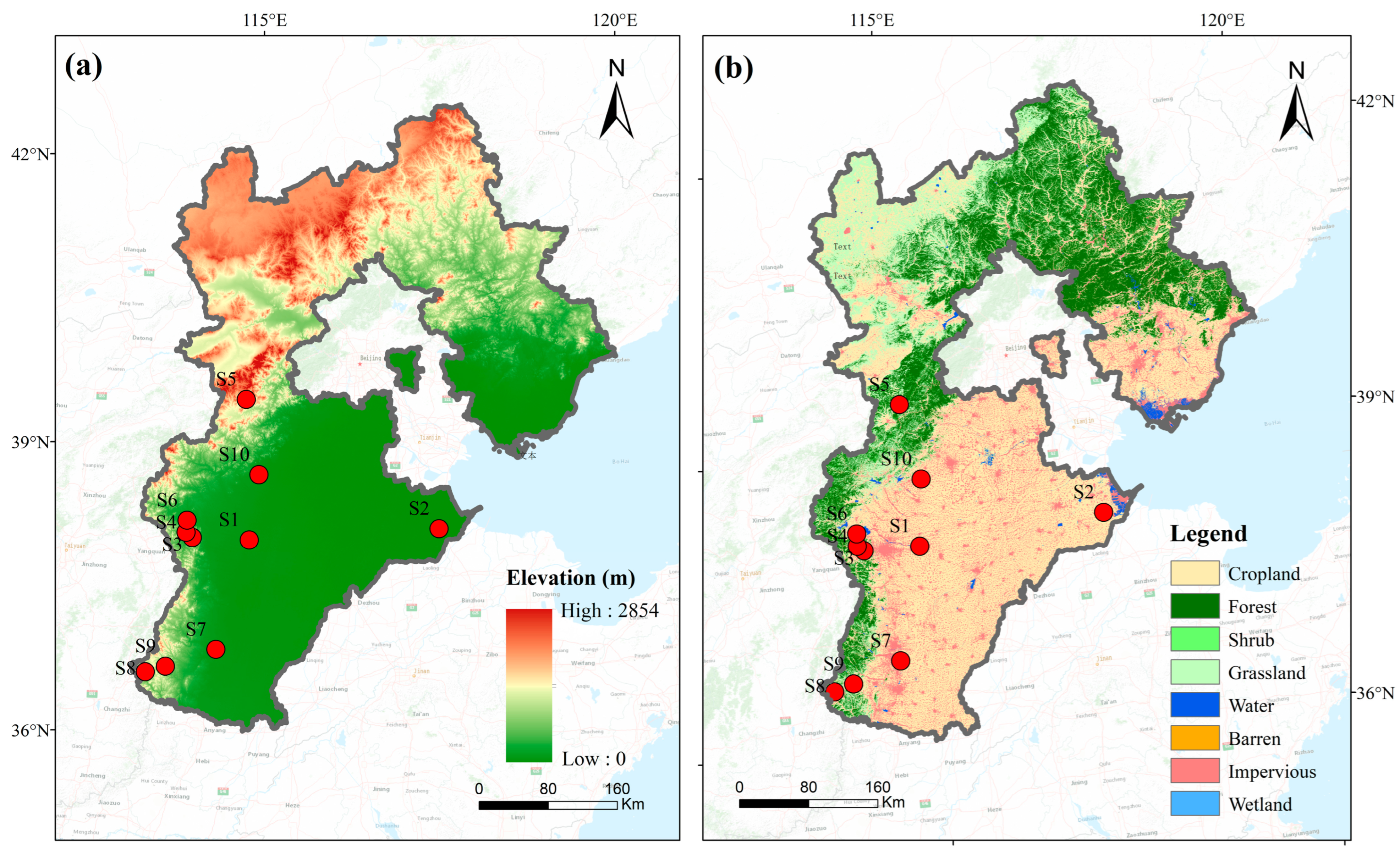
2.1. Study Sites and Data

All 10 PV sites used in this paper are located in Hebei Province, China. This region is characterized by a temperate continental monsoon climate, with an annual average precipitation of 509.2 mm and an average annual sunshine duration of 2449.6 h in 2018, indicating a prolonged period of sunlight and abundant solar resources [24]. The distribution of solar energy resources in Hebei Province typically exhibits a gradual decrease from the northwest to the southeast. The northern regions, located at moderate to high latitudes, are endowed with abundant solar energy resources that generally surpass those in regions at lower latitudes. The annual solar energy in the central part of the province decreases from the edges towards the center in an east–west orientation. The advantageous distribution of solar resources provides a substantial energy foundation for the development of the PV industry in Hebei Province [25].

The PVOD dataset used in this study can be freely downloaded from Github https://github.com/yaotc/PVODataset, accessed on 1 April 2024 [26]. The PVOD has a total of 271,968 records with 10 PV sites and contains numerical weather prediction (NWP) outputs and local measurement data (LMD) from each site at a 15 min temporal resolution. All the sites are located within 36.64–39.52° N, 113.64–117.46° E. The complete dataset covers 348 days and is arranged in chronological order, from 1 July 2018 to 13 June 2019, Local Standard Time (LST). The dataset amalgamates the observed PV power outputs at each site with both in situ measured and NWP model-simulated meteorological parameters, including Global Horizontal Irradiance (GHI) (W/m²), Diffuse Horizontal Irradiance (DHI) (W/m²), temperature (°C), atmospheric pressure (hPa), wind direction (degree), and wind speed (m/s). Furthermore, the dataset encapsulates foundational information pertaining to each PV installation, such as its geospatial coordinates, PV module capacity, surface area, quantity, material composition, and installation orientation. The spatial resolution digital elevation map data used in Figure 1 are from the ASTER GDEMV3 [27] and have a 30 m resolution. These GDEMV3 data can be downloaded from http://www.gscloud.cn (accessed on 1 April 2024), which is provided by the Geospatial Data Cloud site, Computer Network Information Center, Chinese Academy of Sciences. The 30 m spatial resolution Land Cover Data for the year 2020 can be accessed via https://doi.org/10.5281/zenodo.8176941. Furthermore, the land cover is classified into eight categories: (1) Croplands, (2) Forests, (3) Shrub, (4) Grassland, (5) Water, (6) Barren, (7) Impervious, and (8) Wetlands.

The ten PV power sites are predominantly situated in lowland plains and hilly regions (Figure 1a). Their underlying surface composition primarily consists of barren lands, agricultural fields, and grasslands (Figure 1b), featuring sparse vegetation and ample solar irradiance, rendering the terrain conducive to various PV project configurations including ground-mounted stations, agrivoltaic systems, and building-integrated photovoltaics (BIPV). Except for the S2 station in a coastal area, the other installations are mainly in inland regions. Specifically, the sites S3, S4, S5, S6, S8, and S9, located within the vicinity of the Taihang Mountains, exhibit pronounced montane climatic characteristics. Due to their climate features of aridity, scant precipitation, and thin soil, these areas are deemed ideal for the establishment of centralized PV power generation facilities [28]. In contrast, site S2, located near the Bohai Sea and Beijing–Tianjin conurbation and characterized by saline–alkali soils and intertidal flats, presents an ideal environment for the implementation of synergistic aquaculture–PV (APV) systems. Meanwhile, sites S1, S7, and S10, located on inland plains, are influenced by high population densities and widespread agricultural activities. This makes these areas well-suited for the integration of agrivoltaic systems. The spatial arrangement of these installations delineates the topographical complexity inherent to Northern China, encompassing an extensive array of geographic zones. This range extends from the montane attributes discernible at the low mountain sites S5 and S8, through the expansive alluvial floodplains, to the undulating hillocks characteristic of locales such as S3, S4, and S9. Positioned amidst varied geomorphological settings, these locales are identified as prime candidates for PV energy exploitation, attributed to the elevated solar radiative flux and the profusion of solar energy assets available. Furthermore, the significant spatiotemporal heterogeneity observed across these sites underscores the susceptibility of modeling forecasts to predict extreme meteorological events, notably heatwaves. Thus, Section 3.1 will detail the spatiotemporal characteristics of these PV sites and their impact on modeling precision.

2.2. Methods

2.2.1. Selection Criteria for Heatwave and Background Days

To describe the seasonal trends, the data were categorized into spring (March, April, May), summer (June, July, August), autumn (September, October, November), and winter periods (December, January, February). To accurately demarcate heatwave and non-heatwave (i.e., background) conditions, this study employs the meteorological criteria established by the China Meteorological Administration: a period is classified as a heatwave if the daily maximum temperatures reach or exceed 35 °C for at least three consecutive days [29], while other periods during the summer are considered background periods. According to this criterion, only sites S2 and S7 experienced extreme heatwave events of the ten PV power stations. Consequently, this research focuses on the observational data from these two sites during the summer months, segmenting the data into heatwave and background periods.

2.2.2. Machine Learning Algorithms

Given the heterogeneity of regional climates, the efficacy of photovoltaic power generation exhibits significant complexity and diversity [30]. In the context of global warming, the increasing frequency of extreme weather events, particularly heatwave episodes, poses challenges to the accurate forecasting of PV power outputs. To address this issue, this study assesses how well various machine learning models adapt and respond to heatwave and background conditions. Motivated by previous studies [31,32,33,34,35], we employ Random Forest (RF), Decision Tree Regression (DTR), the Support Vector Machine (SVM), the Light Gradient Boosting Machine (LightGBM), Deep Belief Network (DBN), and Multilayer Perceptron (MLP) for model evaluations in our PV power forecasting.

Concurrently, the deployment of the RF Variable Importance Evaluation Methodology [36] is crucial for selecting the meteorological factors that significantly impact the power output of PV systems. Utilizing the feature identification tool of the constructed RF model, this method identifies the importance of our predictors. The importance of each variable is defined by its contribution to the model, with more significant variables exerting a greater influence on the model evaluation results [37]. This technique adeptly discerns the primary features affecting the target variable, accurately pinpointing the factors that decisively influence the efficiency of PV power output. The establishment of the RF Variable Importance Evaluation Method involves the following two steps:

(1) Variable Selection: The output of PV power is a complicated process influenced by various factors, particularly meteorological factors such as solar radiation, temperature, atmospheric pressure, and wind [38,39]. Previous studies [40,41] have shown that GHI, DHI, temperature, atmospheric pressure, and wind are the primary influences on PV power generation. Therefore, this study selects GHI, DHI, temperature, pressure, wind speed, and wind direction for its RF importance analysis.

(2) Construction of RF Variable Importance Evaluation Method: The data from sites S2 and S7 are randomly split into training and testing sets in an 8:2 ratio, respectively. An RF model is then constructed. A grid search algorithm is utilized to identify the optimal combination of hyperparameters, and cross-validation (CV) [42] is employed to enhance the robustness and reliability of the model. The grid search algorithm [43] systematically explores parameter combinations within a defined space, selecting the optimal combination based on performance evaluations. The search range is set as follows: decision tree count (n_estimators) ranging from (100,120,500), maximum tree depth (max_depth) ranging from [None, 15, 20], with the remaining parameters kept as default. Additionally, a 5-fold CV is employed. The optimal hyperparameter combination for both site S2 and S7’s models is n_estimators = 500 and max_depth = None. Finally, the feature identification tool of the RF model is used to evaluate feature importance.

To precisely evaluate the resilience of PV generation systems under the duress of extreme heatwave events, this study adopts a RF regression model as a representative framework for conducting an analytical assessment of PV power output predictions. In the model’s formulation, six meteorological variables were chosen as predictive inputs: GHI, DHI, temperature, atmospheric pressure, wind speed, and wind direction. The PV power output served as the dependent variable of the prediction. The model underwent a rigorous training and validation sequence. The data corpus was partitioned into training and testing subsets in an 8:2 ratio. Specifically, for site S2, the dataset sizes for training during heatwave and background periods amounted to 4991 and 767 records, respectively, with the testing datasets comprising 1248 and 192 records. For site S7, the training datasets contained 2994 records for heatwave periods and 1535 for background periods, with the testing subsets containing 749 and 384 records, respectively. During the division process, a deliberate strategy was employed to maintain the sequential integrity of the data, eschewing randomization to preserve the temporal continuity and comprehensive integrity of the dataset for model training purposes.

To further enhance the predictive accuracy of the RF, this study undertook a meticulous iterative optimization of hyperparameters during the model training phase. Employing a univariate adjustment strategy, namely Grid Search [44], this study specifically optimized the hyperparameters of the RF models for both the S2 and S7 sites under heatwave and background conditions. The optimization results revealed the optimal parameter configurations for the background model and heatwave model at site S2 and site S7, which are shown in

Table 1. The hyperparameters of the RF at sites S2 and S7.

Station	Period	n_Estimators	Max_Depth	Min_Samples_Split	Min_Samples_Leaf
S2	background	130	10	6	5
	heatwave	100	10	8	5
S7	background	190	16	6	3
	heatwave	190	18	2	14

.

2.2.3. Metrics for Evaluating Model Performance

In this investigation, the evaluative framework for assessing the predictive power of the model in forecasting PV power output amidst heatwave and background scenarios contains three pivotal statistical indices: the coefficient of determination (R²), root mean square error (RMSE), and mean absolute error (MAE). Three indicators can be expressed as follows [45]:

$$R^2=1-\frac{{\sum _{i=1}^n\left(y_i-{\widehat{y}}_i\right)}^2}{{\sum _{i=1}^n\left(y_i-\overline{y}\right)}^2}$$

(1)

$$RMSE=\sqrt{\frac{1}{\overline{n}}{\sum }_{i=1}^n{\left(y_i-{\widehat{y}}_i\right)}^2}$$

(2)

$$MAE=\frac{1}{n}{\Sigma }_{i=1}^n\left|y_i-{\widehat{y}}_i\right|$$

(3)

Within these equations, $n$ denotes the number of samples, $y_i$ represents the genuine observed value for the $i^{th}$ sample, ${\widehat{y}}_i$ signifies the predicted value for the $i^{th}$ sample, and $\overline{y}$ is the mean of all observed values. $R^2$ illustrates the proportion of variance in the dependent variable that is accounted for by the independent variables, with values ranging from 0 to 1. Values closer to 1 indicate a higher model fit quality, while those approaching 0 suggest a lack of fit. The RMSE is the square root of the average of the squared differences between the observed and predicted values, reflecting the standard deviation of the prediction errors and quantifying the discrepancy between model predictions and actual observations. A smaller RMSE value denotes smaller errors in model simulations. The MAE calculates the average of the absolute differences between the observed and predicted values, providing a direct measure of the average magnitude of prediction errors. Unlike the RMSE, the MAE does not disproportionately penalize larger errors, thus ensuring a more balanced assessment of error magnitudes.

2.2.4. Pearson Correlation Coefficient Analysis

In statistics, the Pearson correlation coefficient (or Pearson product–moment correlation coefficient) measures the linear correlation between two variables [46]. It ranges between −1 and +1, where +1 indicates a perfect positive linear correlation, 0 indicates no linear correlation, and −1 indicates a perfect negative linear correlation. The definition of the Pearson correlation coefficient $r$ is as follows:

$$r=\frac{\sum _{i=1}^n(x_i-\overline{x})(y_i-\overline{y})}{\sqrt{{\sum }_{i=1}^n{(x_i-\overline{x})}^2}\sqrt{{\sum }_{i=1}^n{(y_i-\overline{y})}^2}}$$

(4)

Within the equation above, $n$ is the sample size; $x_i$ and $y_i$ are the individual sample points indexed with $i$; $\overline{x}$ is the sample mean, representing $\frac{1}{n}{\Sigma }_{i=1}^n{x}_i$; and the same is the case for $\overline{y}$.

3. Results and Discussion

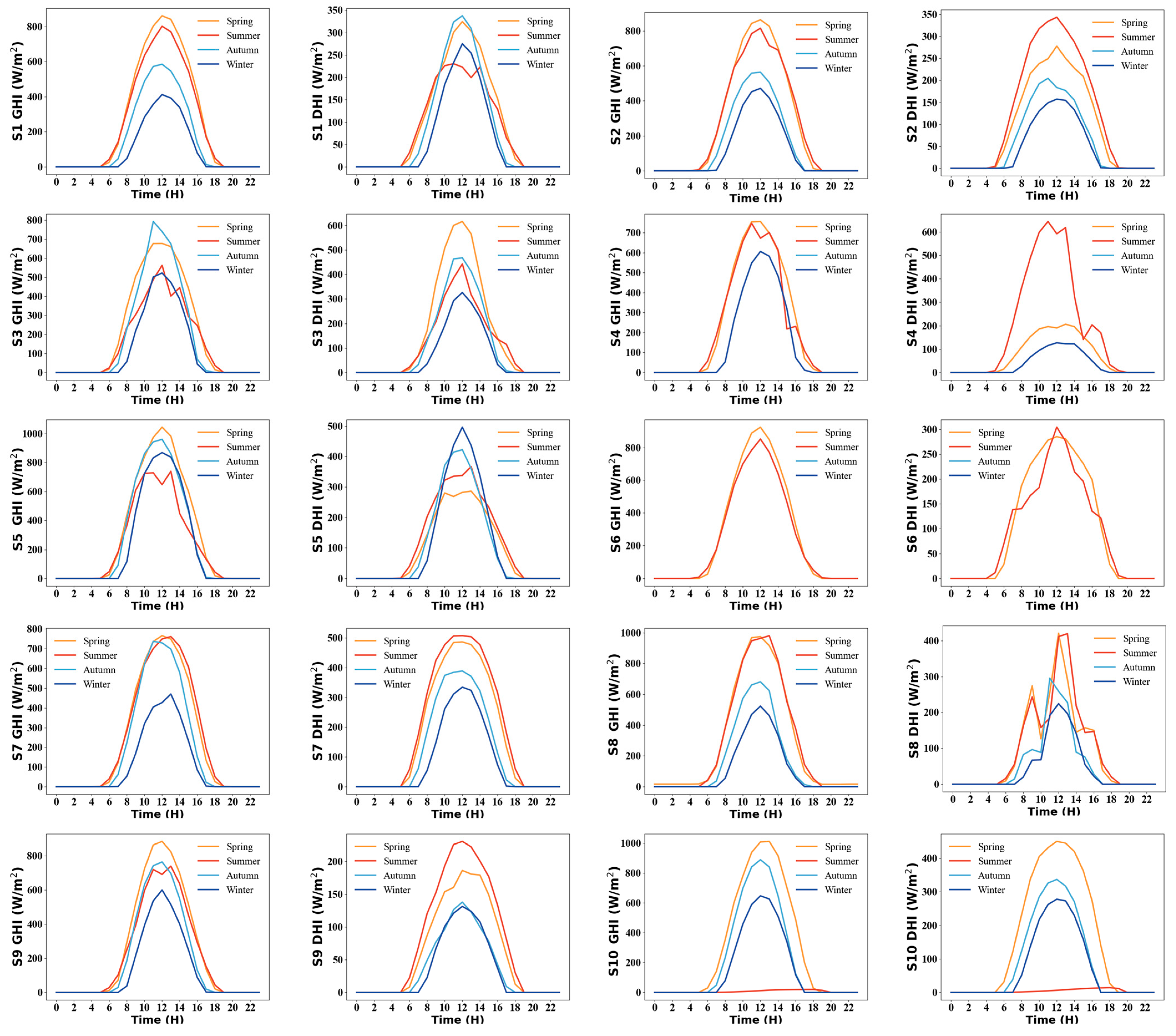
3.1. Spatio-Temporal Patterns of Solar PV Energies

This study conducted a spatiotemporal analysis of the daily PV power output across ten PV stations, revealing that all sites exhibit a pronounced diurnal pattern in their power output, as illustrated in Figure 2. Specifically, the power output demonstrates a gradual increase from dawn (06:00) to noon (12:00) and subsequently decreases from noon to dusk (20:00), forming a characteristic inverted “U”-shaped diurnal profile. Notably, the power output at individual PV stations remains consistently at zero during the nocturnal period (20:00 to 05:00 the following day). This is attributable to the diurnal rotation of the Earth, which results in the reduction of total solar irradiance, direct irradiance, and diffuse irradiance to zero during this interval. Despite the uniformity in diurnal trends across all PV sites, there is a significant variation in the specific power output values between sites. For instance, the peak daily power output at site S6 can exceed 25 MW, markedly surpassing that of site S1 (approximately 4 MW). This discrepancy is likely due to the superior geographical positioning and lower topographical obstructions at site S6, whereas site S1, located in a relatively low-lying area and overshadowed by surrounding mountains, experiences diminished solar irradiance [47].

Furthermore, the ten PV stations within the study area exhibit pronounced seasonal variability. In spring and summer, the PV power output at each site is significantly higher than in autumn and winter, due to their higher solar elevation angles, resulting from their geographic locations. Notably, except for sites S7 and S10, the peak daily power output at most stations predominantly occurs in spring.

Figure 3 depicts the diurnal patterns of GHI and DHI at 10 PV sites across four seasons. The daily peak values of GHI and DHI at most sites are typically observed in spring (about 677–1045 W/m² for GHI and 206–615 W/m² DHI), followed closely by summer. The availability of valid data at site S10 was significantly affected by consecutive cloudy or rainy days [48], leading to a notably lower GHI and DHI in summer. The temperature at all sites exhibits a distinct seasonal pattern, peaking in summer (about 25–34 °C), followed by spring, autumn, and winter (Figure 4). Generally, summer is characterized by intensified solar radiation and higher temperatures due to the Earth’s axial tilt and the movement of the solar declination.

This period is characterized by intensified solar radiation due to the Earth’s axial tilt and the movement of the solar declination, significantly outstripping other seasons. Based on the trend of the diurnal variation curves, temperature exhibits a distinct seasonal pattern, peaking in summer, followed by spring, autumn, and finally winter, with a gradual decline in temperature. However, except for at sites S2 and S5, the peak daily power outputs in winter are observed to be the lowest throughout the year, which reflects the geographic characteristics of lower solar elevation angles and weaker solar irradiation seen during this season. Conversely, the lowest peak daily power outputs at sites S2 and S5 occur in summer, potentially linked to seasonal variations in local geographic conditions such as atmospheric transparency and cloud cover [49]. The peak daily PV power output at each site rises from 06:00 to 12:00 LST and decreases from 12:00 to 20:00 LST. The seasonal differences are evident, with the most pronounced disparity around noon. This phenomenon reveals how geographic factors, like changes in the Earth’s axial tilt, cause variations in the sunlight’s duration and intensity across seasons. It also highlights the unique responses of PV sites in the region to these seasonal changes.

Considering the diversity of their geospatial distribution, the ten PV stations encompassed in this study exhibit significant spatial climatic heterogeneity. Against the backdrop of global climate change, China is encountering increasingly frequent and intense heatwave events [50], leading to pronounced disparities in the response of PV stations situated in different geographic locations to heatwaves. Influenced by topography, PV sites located in foothill and coastal areas are more susceptible to the severe impact of heatwaves. In contrast, regions at higher elevations (such as sites S3, S4, S5, S6, S8, and S9) experience relatively milder effects during heatwaves [51].

In summary, influenced by the interplay between topographical characteristics and regional microclimatic conditions, PV stations within Hebei Province exhibit distinct diurnal patterns and seasonal power fluctuations. Specifically, the variability in their geographical locations and the diversity of the terrain contribute to the significant variations in PV power output among different stations. These spatiotemporal dynamic characteristics underscore the profound impact of extreme climatic events, such as heatwaves, on the performance of PV systems. In light of this, this study delves into the impact mechanisms of heatwave events on PV power output and thoroughly analyzes their underlying influencing factors, aiming to provide a scientific basis for the optimized operation and maintenance of PV systems and their adaptation to extreme climate events.

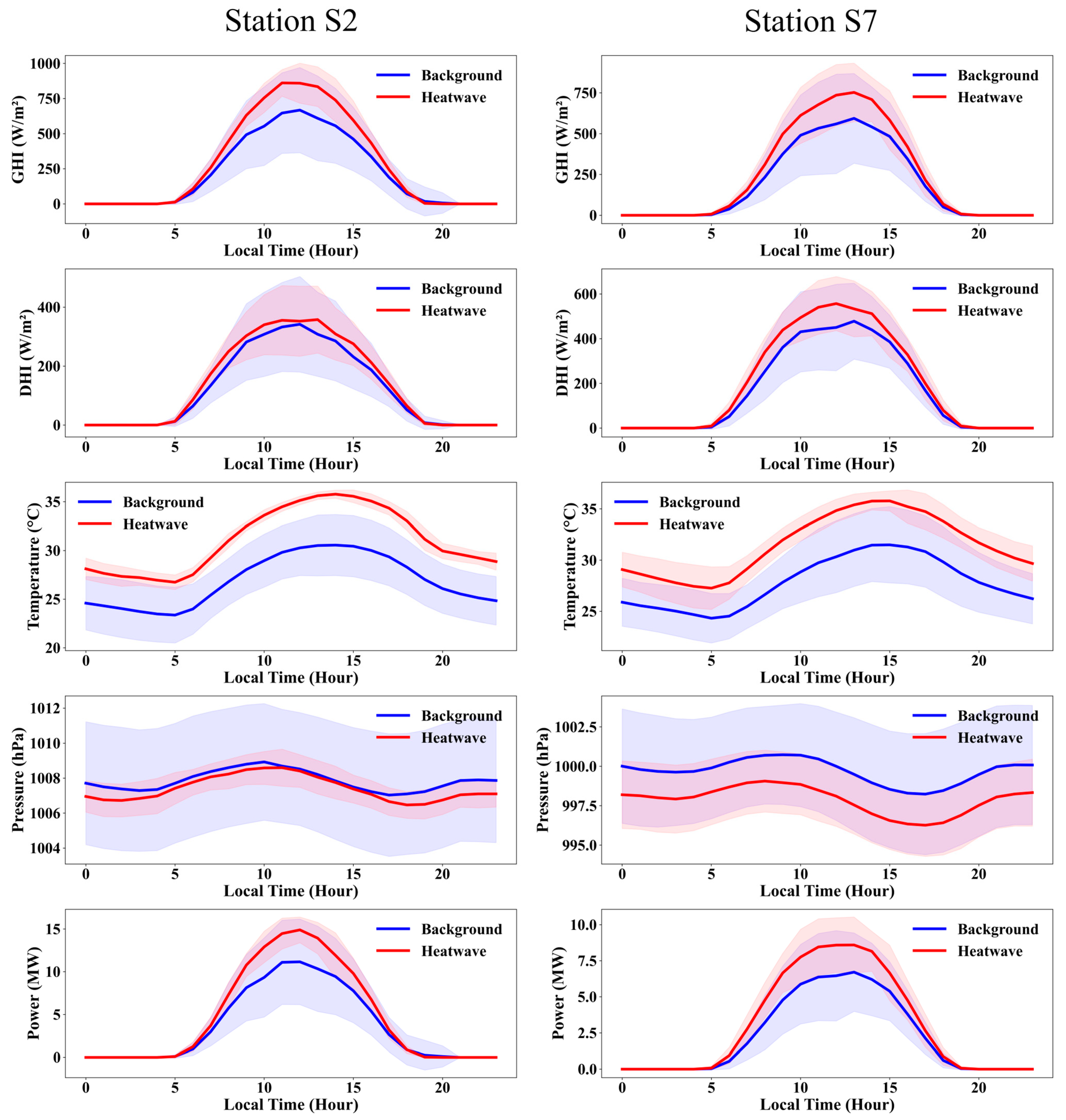
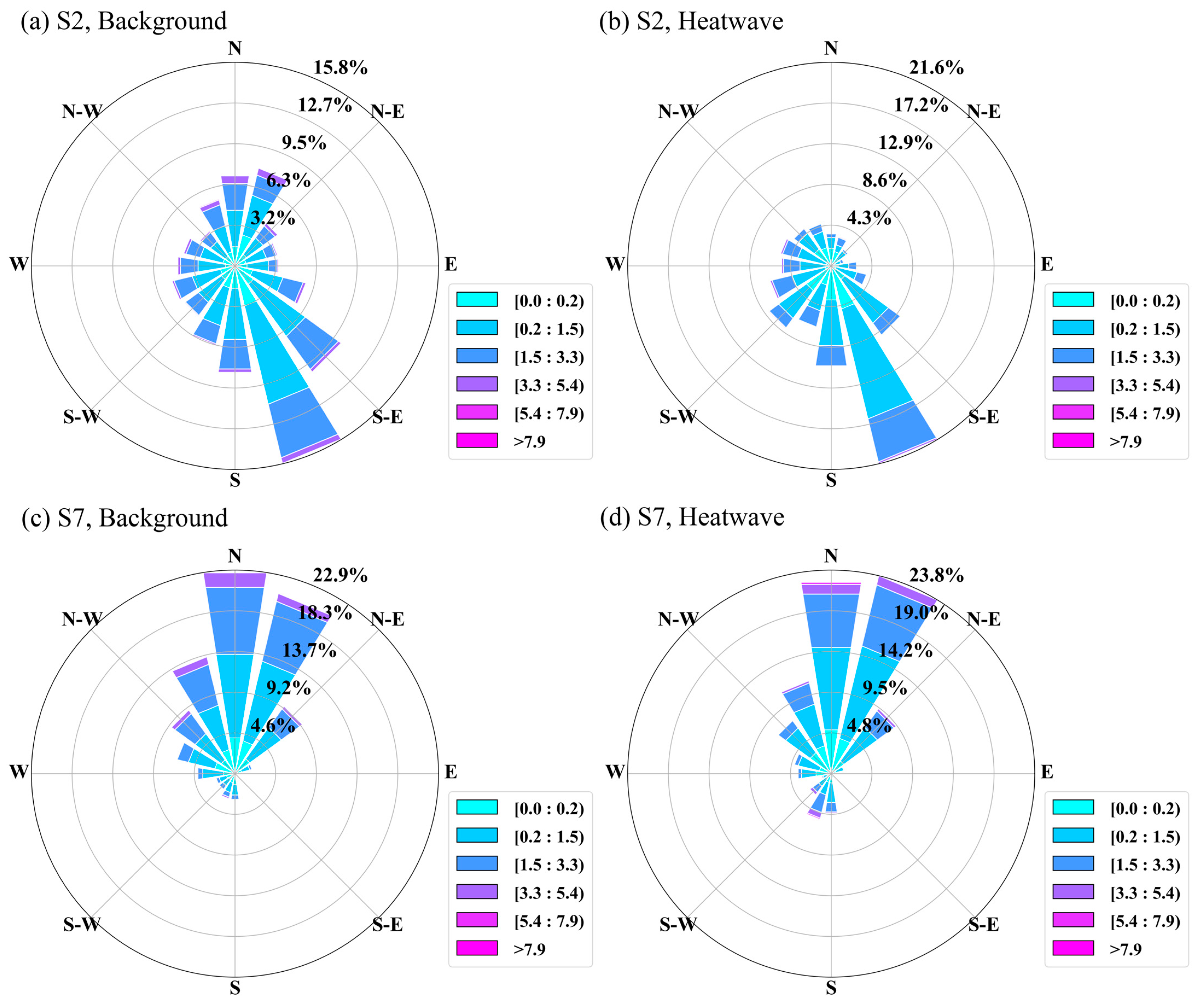
3.2. Meteorological Conditions under Heatwave and Background Days

Figure 5 illustrates the meteorological conditions and their relationship to PV power generation at sites S2 and S7 under heatwave and background conditions. This study reveals that, during heatwave periods, both stations exhibit significantly elevated levels of GHI, DHI, temperature, and PV power output, compared to during background periods. Additionally, atmospheric pressure levels are notably lower under heatwave conditions. The variability of meteorological conditions during heatwaves tends to be more stable, and diurnal trends exhibit consistency irrespective of the presence of a heatwave. Specifically, from dawn at 06:00 to noon at 12:00, the discrepancies in GHI, DHI, and PV power output progressively amplify, while from noon to dusk at 20:00, these discrepancies gradually diminish, with the variance being particularly pronounced at midday. For instance, during heatwave conditions, the midday peak at site S2 showed a 28.92% increase in GHI, a 16.15% rise in DHI, and a 33.50% surge in PV power output compared to background periods. Meanwhile, at site S7 under heatwave conditions, the increases in midday peak GHI, DHI, and PV power output were 31.45%, 23.70%, and 32.90%, respectively, relative to background conditions, underscoring the significant impact of varying meteorological conditions on PV power generation.

In the investigation of the urban heat island effect at sites S2 and S7 and its impact on the local temperature field, it was observed that the temperature differentials between heatwave and background conditions exhibit significant temporal distribution characteristics within the diurnal cycle. Specifically, the temperature range at site S2 during heatwave periods was primarily concentrated around 14:00 in the afternoon, at which time the temperature was significantly, 17.05%, higher compared to background conditions. At site S7, the peak temperature differential occurred at noon (12:00), with temperatures under heatwave conditions being 14.83% higher than those during background periods. Regarding the minimum temperature differential, site S2 recorded its lowest temperature at 02:00 during the night, amounting to only 13.76% of that during background periods, while site S7 recorded its minimum temperature differential at 04:00 in the morning, accounting for 11.20% of background conditions.

In the comparative analysis of wind field characteristics during heatwave and background periods (Figure 6), it was observed that wind speeds during heatwaves are generally lower than those during background periods at the same geographical coordinates. This phenomenon is particularly evident in the wind rose diagrams of sites S2 and S7. At site S2, the proportion of higher wind speeds from the south (S) increased significantly during heatwave periods (Figure 6b) compared to background periods (Figure 6a). This was particularly true at higher wind speed thresholds (represented by the light purple and pink areas, indicating wind speeds exceeding 5.4 m/s), where the frequency of occurrences markedly increased during background periods. The situation at site S7 was even more pronounced, with significant differences in wind speed and direction between the background (Figure 6c) and heatwave (Figure 6d) periods, where the proportion of higher wind speeds from the south significantly increased during heatwave periods.

Moreover, both sites exhibited a higher proportion of low wind speeds from the north (N) during both background and heatwave periods. However, during heatwaves, the proportion of higher wind speeds from the northeast increased relative to the background periods (represented by the dark blue and blue areas). This is associated with increased atmospheric stability during heatwaves, leading to a reduction in vertical wind speed components and an increase in horizontal wind speed components in specific directions [52]. Across all heatwave scenarios, the frequency of winds in the moderate wind speed range (purple area, with speeds between 3.3 and 5.4 m/s) was relatively low. This reflects that the insufficient thermal convection caused by surface radiative heating during high-temperature periods in summer fails to generate strong wind field dynamics [53]. Overall, irrespective of heatwave or background conditions, the wind speeds in summer generally remain at lower levels. This closely related to the atmospheric stability induced by seasonal high-pressure systems [54].

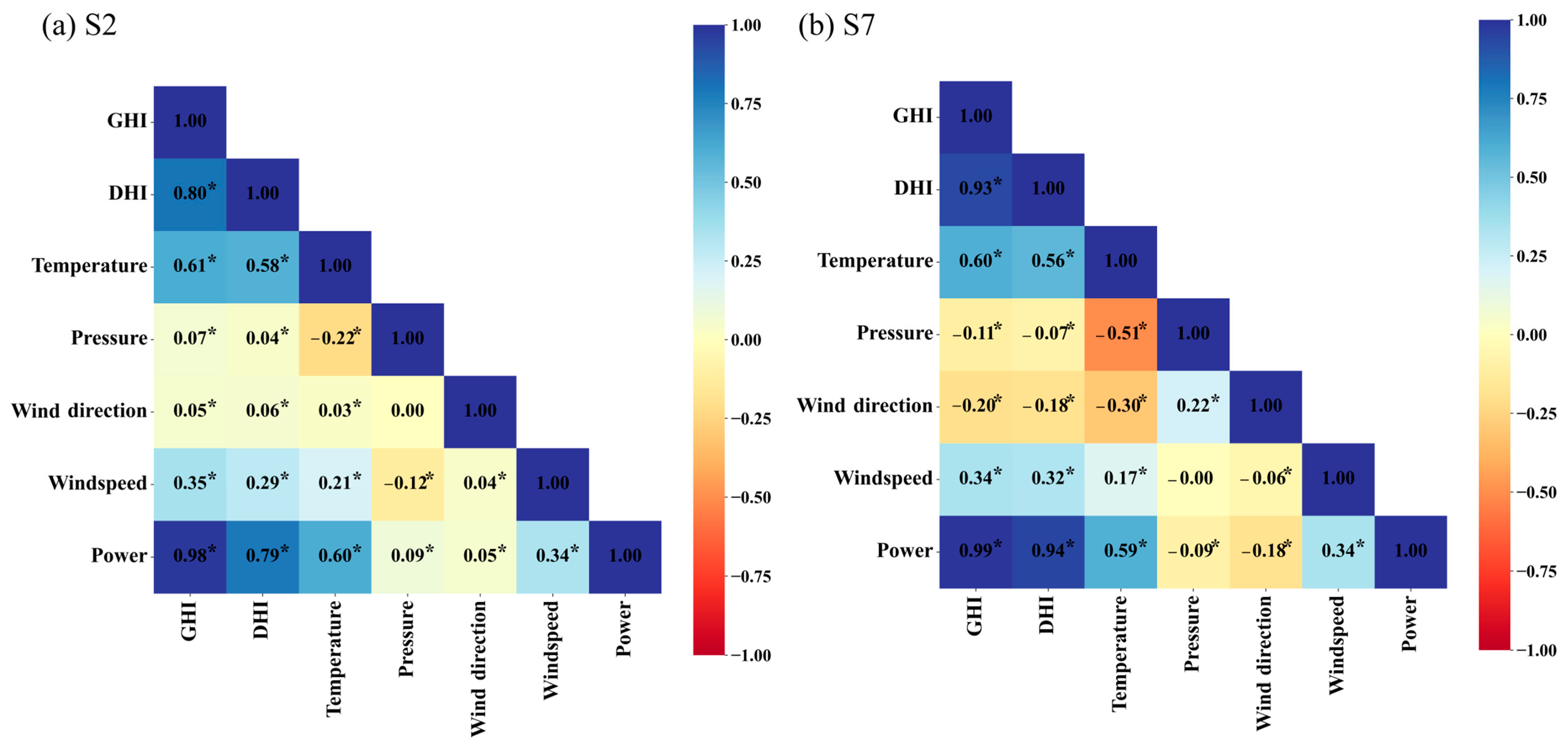
3.3. Driving Factors of PV on a Seasonal Scale

Under identical wind speed conditions, the power output of photovoltaic systems is closely linked to the microclimatic conditions of their locations [55]. As demonstrated in Figure 7, the calculation of Pearson correlation coefficients between the PV power output at sites S2 and S7 and various climatic parameters reveals the sensitivity of photovoltaic systems to meteorological variables. Particularly in summer, which is dominated by the climatic backdrop of subtropical high-pressure systems and consequent heatwave events, the sensitivity of PV systems to meteorological factors notably increases. Our Pearson correlation coefficient analysis indicates a significant positive correlation between PV power output and both GHI and DHI. This relationship directly mirrors the energy conversion mechanism of PV panels—solar radiation is absorbed by the panels and converted into electrical energy, with the conversion efficiency being proportional to the incident radiation [56]. Consequently, higher radiation intensities correlate to increased power outputs from PV systems, and vice versa.

It is noteworthy that a significant positive correlation is also observed between PV power output and ambient temperature. Ambient temperature, which reflects the level of heat in the air, is directly influenced by and indicative of changes in solar radiation. Under clear sky conditions, an increase in ambient temperature is typically due to heightened solar radiation intensity and reduced attenuation during its transmission. Consequently, higher daily average temperatures—within a moderate range from a low point (e.g., near the freezing point) up to approximately 30 °C to 40 °C, without exceeding 45 °C—correlate to increased photovoltaic power output [57,58,59]. Therefore, under extreme climatic conditions, particularly during high-temperature heatwave events, the sensitivity of the PV system’s power output characteristics to meteorological factors is heightened. This is partly attributable to the stability and expansion of subtropical high-pressure systems, as well as orographic-induced katabatic flows. They collectively contribute to increased occurrences of clear weather and elevated temperatures. Consequently, this augments the energy conversion efficiency of PV systems, especially in regions experiencing intense solar radiation.

Figure 8 elucidates the hierarchical ranking of the impact of climatic elements on PV power performance within the study area. An importance analysis conducted using the RF algorithm indicates that, across the two sites involved, GHI contributes most significantly to the power output of PV systems, with its influence weight exceeding 0.94, markedly higher than that of DHI, which ranked second. Specifically, the influence weight of DHI at site S2 is 0.016, while at the inland site S7 it reaches 0.049. Additionally, the Pearson correlation analysis in Figure 7 also reveals a similar trend, with a correlation coefficient of 0.79 at site S2 and 0.94 at site S7. This finding reveals that, during summer, the inland region where S7 is located, in comparison to site S2, exhibits lower atmospheric transparency and a higher atmospheric scattering particle concentration, thereby enhancing its contribution to diffuse radiation [60]. The topographical configuration surrounding site S7, a mountainous encirclement, induces an orographic blockage effect that restricts the atmospheric dispersion of gases and particulates. This phenomenon is further compounded by a humidity feedback mechanism attributable to widespread irrigation practices within the region’s agricultural expanses [61], amplifying the localized greenhouse effect during the summertime. Consequently, this leads to a diurnal PV power generation profile in the summer that closely parallels that observed during the spring season for this site (Figure 2). It also creates a distinct seasonal PV power output pattern unique to the S7 area.

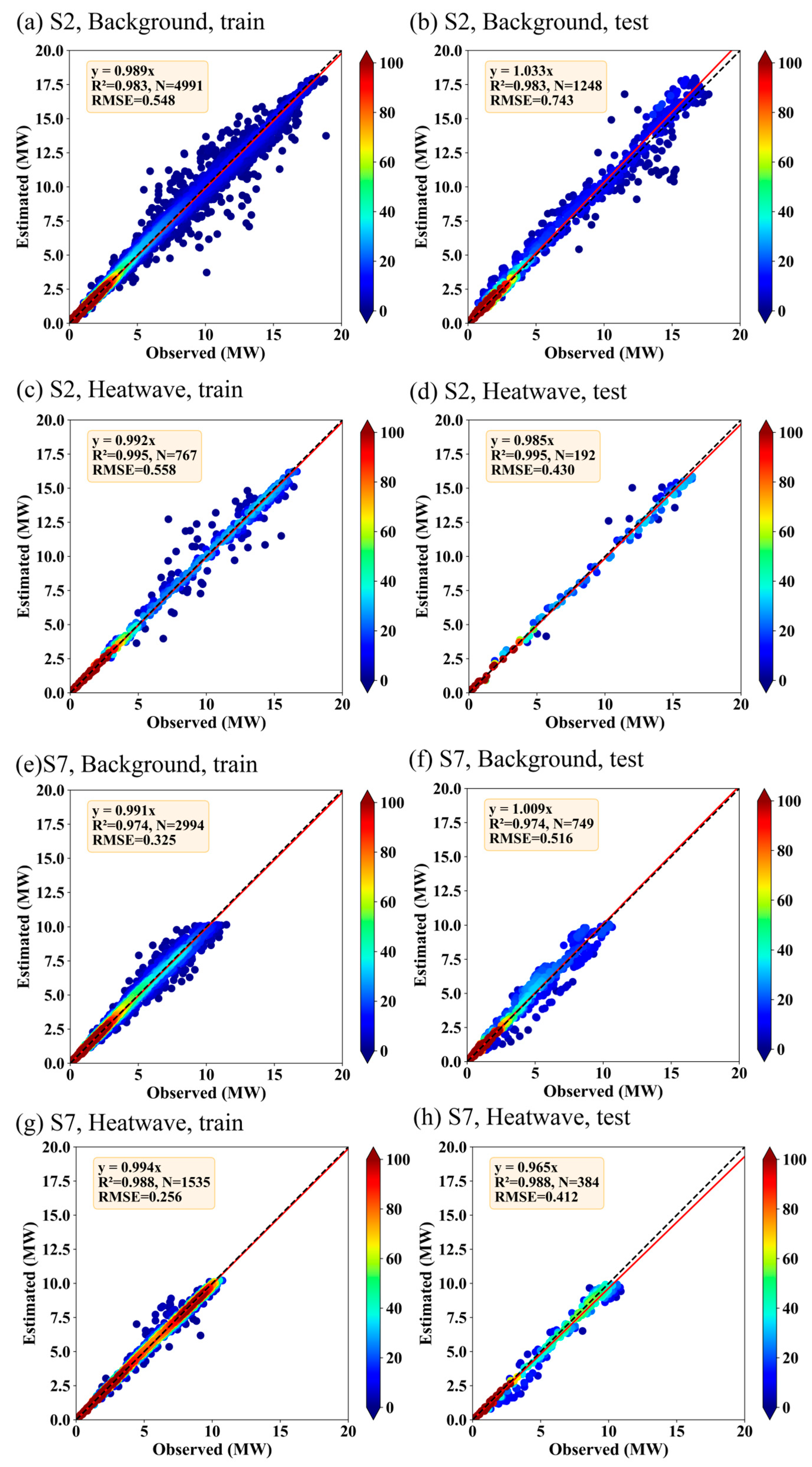
3.4. Random Forest Model Evaluation

The scatter plots depicted in Figure 9 employ Gaussian Kernel Density Estimation (KDE) to represent the distribution density of the data points, reflecting the concentration of sample points per unit area. The predictive outcomes of the model indicate that, for both PV sites, the R² values achieved during heatwave periods are significantly higher than those during background periods, 0.995 and 0.988, respectively, while the corresponding RMSE values are notably lower in these heatwave conditions, at 0.43 and 0.41, respectively. In the prediction of background period data, the scatter plots exhibit deviations towards the axes. This indicates limitations in the model’s predictive capability of PV power during background periods. Conversely, under heatwave conditions, the predicted scatter in Figure 9d is significantly concentrated near the line of equality (1:1 line), with a similar trend observed in Figure 9h. This finding suggests that the RF regression model exhibits heightened sensitivity and accuracy in predicting the power output of PV systems under heatwave conditions, demonstrating a particularly superior predictive performance during heatwave periods. This further underscores its potential for high-precision forecasting in the context of extreme climatic conditions.

The analysis presented in Figure 10 reflects a comparison between the predicted and actual observed PV power outputs over a 24 h cycle for a specific day within the selected test dataset. Under background conditions, the RF prediction models for sites S2 (Figure 10a) and S7 (Figure 10c) are able to closely match the actual power data at most time points, yet significant prediction deviations are observable during certain intervals. In contrast, under heatwave conditions, the predictive performance for both sites S2 (Figure 10b) and S7 (Figure 10d) is notably enhanced. The prediction curves accurately trace the fluctuation trends of the actual power data and there is a significant reduction in prediction errors. This indicates the models’ ability to precisely capture the PV power fluctuation patterns occurring under extreme climatic conditions. Upon comprehensive evaluation, the RF models exhibit commendable performances across all four scenarios, with minor predictive errors. Overall, they successfully delineate the diurnal pattern of PV power, particularly under heatwave conditions. The close alignment between the predicted and actual data underscores the models’ high adaptability and robustness to extreme climatic variations, as well as their more acute and precise predictive responses compared to under background conditions.

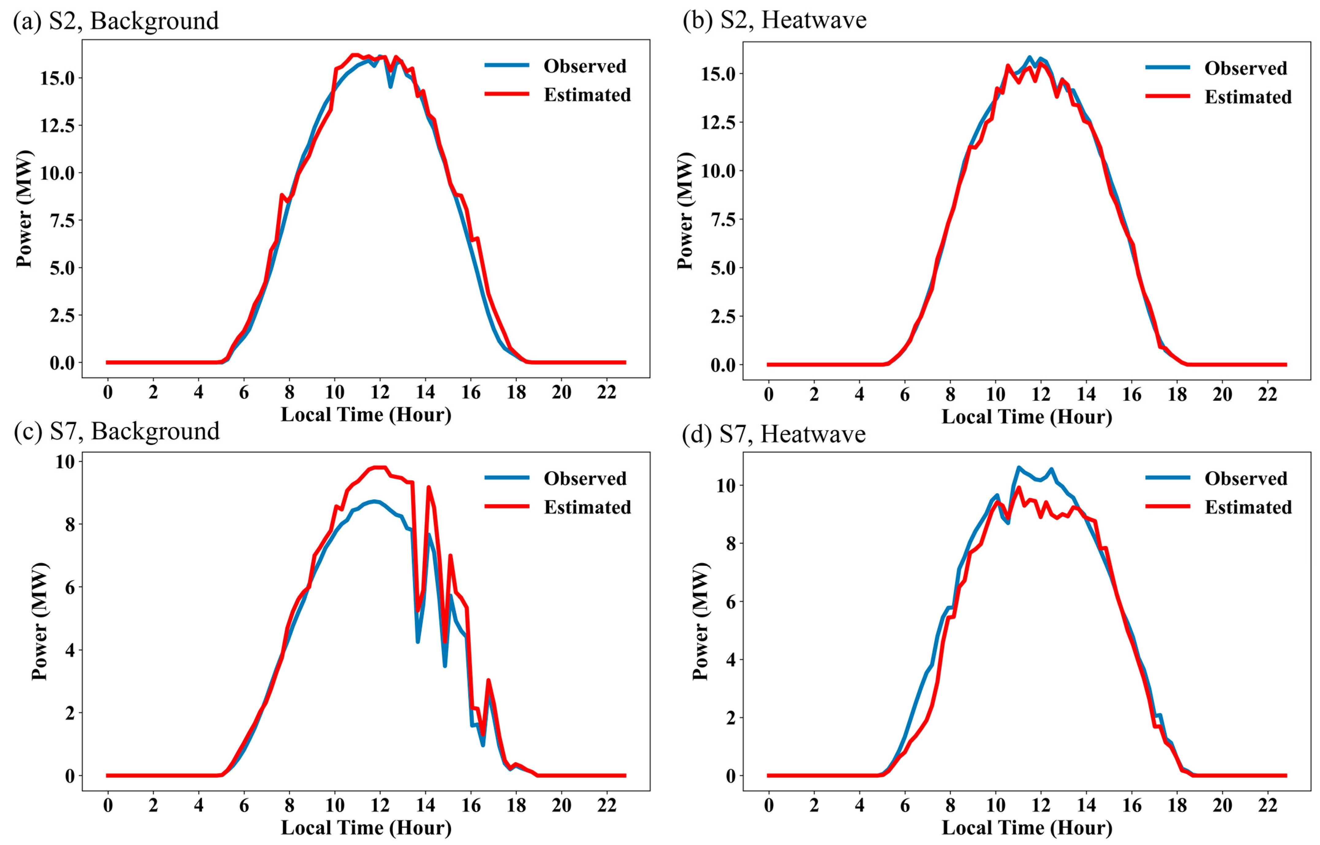
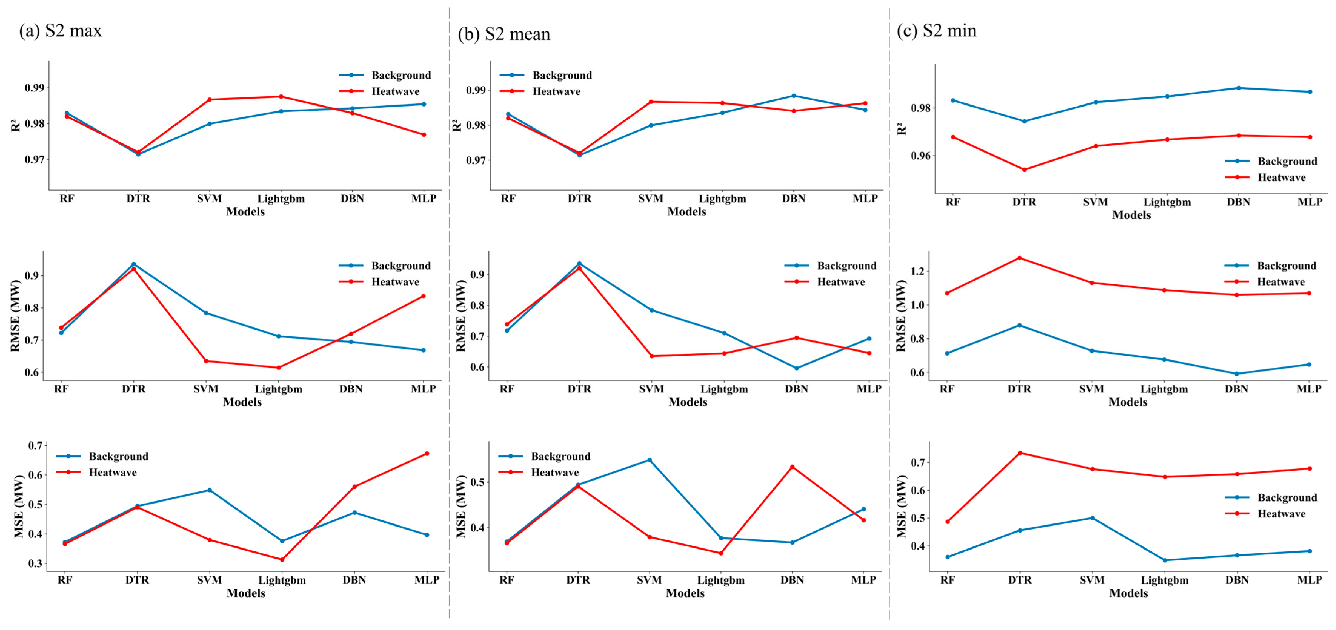
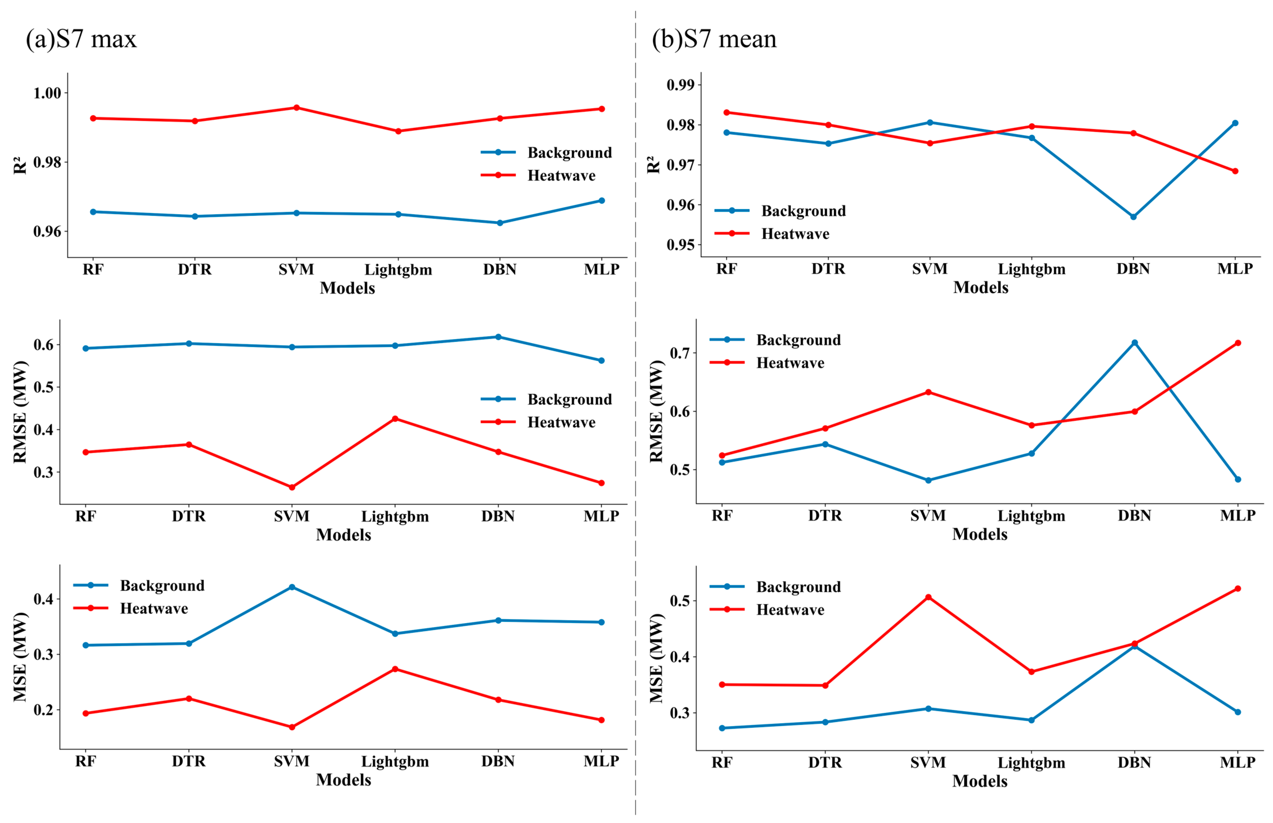
3.5. Performance of Diverse Models under Heatwave and Non-Heatwave Conditions

This study thoroughly assesses how different machine learning models perform during heatwave conditions. It encompassed DTR, the SVM, and the LightGBM, alongside DBN and MLP, within the deep learning paradigm. These models were developed and calibrated within a Python computing environment, leveraging the capabilities of the scikit-learn and PyTorch libraries. To ascertain peak performance across the algorithmic spectrum, a comprehensive hyperparameter optimization process was undertaken for each model to achieve an ideal configuration.

In the model optimization process, various strategies were employed in this study to precisely adjust key hyperparameters, ensuring the efficient performance and generalization capability of the models. Specifically, for DTR, a grid search technique was utilized to fine-tune the parameters, including the max_depth, min_samples_leaf, and min_samples_split, with ranges of (1,20), (1,20), and (2,20), respectively, resulting in the construction of high-performing models. For the LightGBM, the meticulous definition of parameter search ranges, including n_estimators from 100 to 500, max_depth from 5 to 40, maximum number of leaf nodes (num_leaves) from 50 to 300, and the minimum number of samples required to form a leaf node (min_child_samples) from 15 to 50, was conducted to enhance the model’s generalization performance. The SVM underwent rigorous parameter tuning, resulting in a combination of the regularization parameter (C) set at 100.0 and the kernel width (gamma) at 0.01, achieving a balance between model complexity and generalization. The MLP utilized a Bayesian optimization algorithm to efficiently explore the parameter space and included hidden layer sizes (hidden_layer_sizes) from 100 to 500, a batch_size from 10,000 to 30,000, and a maximum number of iterations (max_iter) from 100 to 500, maximizing the potential performance of the model. As for the DBN configuration, a structure comprising two hidden layers (with 400 and 200 neurons, respectively) was designed, with 50 rounds of pre-training iterations and 200 rounds of fine-tuning iterations scheduled. Through these comprehensive hyperparameter optimization measures, the models were sure to achieve an optimal performance tailored to specific tasks. The detailed outcomes of this comparative analysis are presented in Figure 11.

In the PV power prediction analysis of site S2, ensemble learning methodologies such as RF and LightGBM displayed pronounced responsiveness and exceptional adaptability within the context of heatwave scenarios. Their prediction results are comparable to traditional machine learning methods such as DTR and SVM. This is evident from their high R² and low RMSE and MAE. Notably, RF achieved an exceptional performance on the test set for site S2, with an R² of 0.995 and RMSE and MAE values of 0.19 MW and 0.21 MW, respectively. On the other hand, within the realm of deep learning architectures, DBN manifested a suboptimal performance under analogous heatwave conditions, as indicated by its reduced R² and escalated RMSE and MAE, highlighting its predictive constraints under such extreme weather conditions. The MLP exhibited a moderate adaptation capacity to the extreme climatic shifts presented by heatwaves. Regarding site S7, both RF and LightGBM consistently demonstrated heightened adaptability and precision in their forecasting under severe heatwave circumstances, a claim substantiated by their distinctly superior R² metrics and markedly inferior RMSE and MAE values in comparison to alternate models. In terms of their performance metrics, the RF model achieved an R² value of 0.988 and the RMSE and MAE for the RF model were calculated to be 0.41 MW and 0.22 MW, respectively. Similarly, the LightGBM also reported an R² value of 0.988, with an RMSE of 0.41 MW and an MAE of 0.24 MW. In relative terms, the performance of the SVM was found to be comparatively weaker, whereas DTR, DBN, and the MLP did not exhibit significant efficacy in responding to the extreme climatic conditions presented by the heatwave scenario.

In a comprehensive assessment, the RF and LightGBM models consistently exhibited superior efficacy across both examined scenarios, whereas the MLP predominantly underperformed. These findings suggest that, within the dataset utilized for this investigation, the RF and LightGBM models manifested pronounced adaptability and precision in forecasting under severe meteorological phenomena such as heatwaves, distinguishing themselves from comparable models. This highlights the superiority of ensemble learning algorithms in navigating the complex and nonlinear dynamics of PV power forecasting under climatic influences.

When comparing the predictive performance of different models (such as DBN and SVM) at different sites (S2 and S7), we observed a significant sensitivity to data characteristics. Specifically, DBN exhibited higher predictive accuracy during background periods at site S2, while its performance was more prominent during heatwave periods at site S7. Similar phenomena were observed with the SVM, which had significant performance variation across both sites due to differing dataset characteristics. In contrast, both the DTR and MLP models demonstrated improved predictive performances during heatwave periods compared to background periods across both datasets, albeit with noticeable differences in the magnitude of the improvement between the S2 and S7 sites. For MLP, the increase in PV power prediction accuracy during heatwaves at S2 was approximately 0.002, whereas at S7 it reached a significant improvement of 0.01. Similarly, DTR exhibited an increase of approximately 0.01 in predictive accuracy for heatwaves at S2, while the improvement was smaller at S7, approximately 0.004. These findings suggest that DBN and SVM heavily rely on data characteristics during prediction, necessitating fine-tuning based on specific dataset features. While the DTR and MLP models demonstrate an overall good predictive performance during heatwave periods, optimization strategies across different sites need to be tailored to their specific dataset performances. The insights derived underscore the criticality of model selection tailored to specific climatic exigencies when deploying machine learning and deep learning frameworks for PV power forecasting, which is particularly pertinent in the face of extreme climate events that pose significant perturbations to power systems. Additionally, the discerned impact of extreme weather conditions on the performance of predictive models elucidates the imperative for augmented model optimization to bolster their predictive accuracy in the face of climatic extremities.

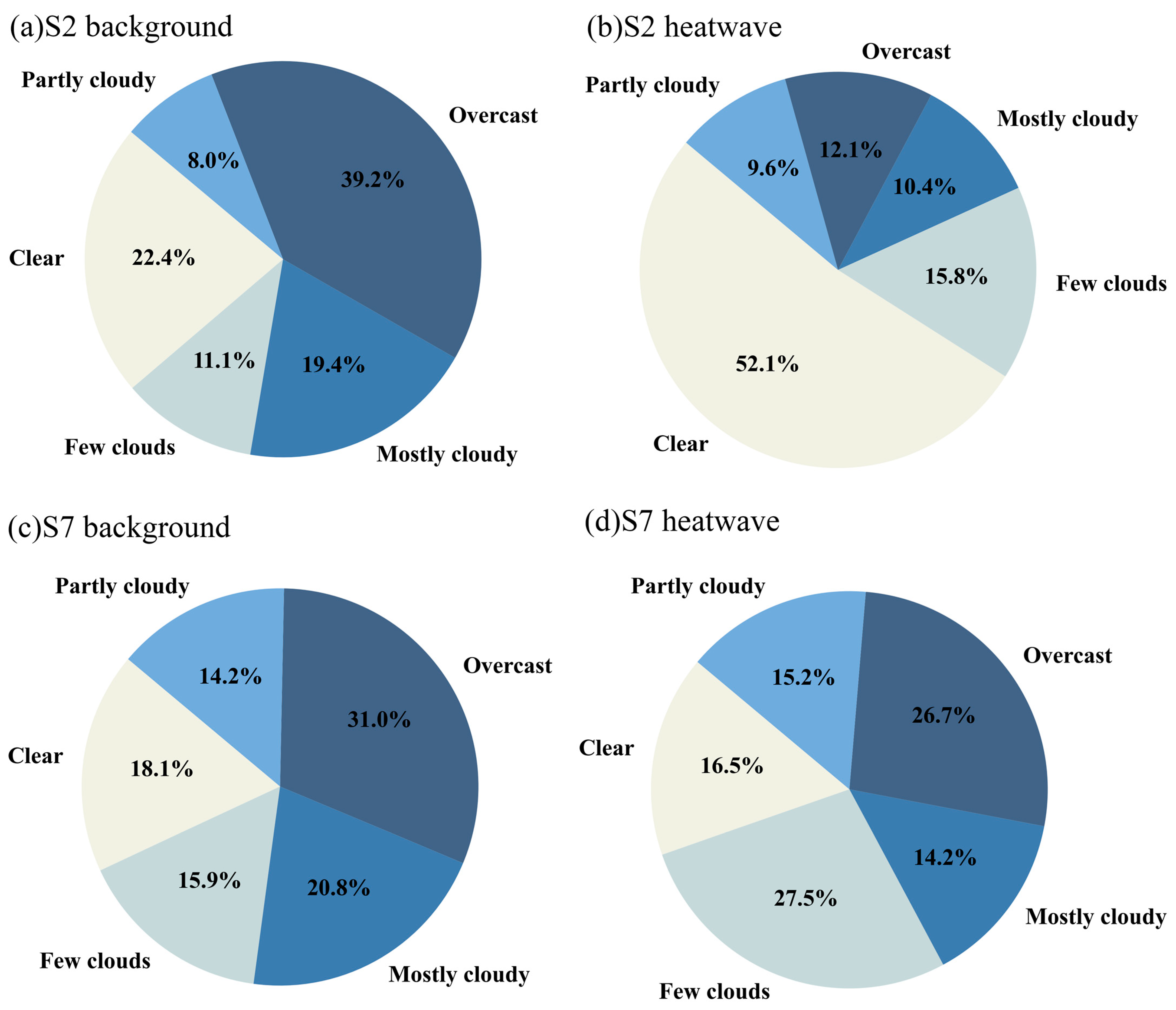
3.6. The Impact of Cloud Cover on the Prediction of Photovoltaic Power Generation

In the field of PV power generation, the output PV power is influenced by a combination of various environmental factors. These factors not only include the intensity of the solar radiation, ambient temperature, changes in atmospheric pressure, and the effects of wind speed and direction, but also the amount of cloud cover, which is an important factor that cannot be ignored [62,63]. Changes in cloud cover directly affect the intensity of the solar radiation reaching the ground, thereby significantly impacting the power output of PV power plants.

In recent years, with in-depth research on the efficiency and stability of PV power generation systems, the impact of cloud cover on PV power has increasingly attracted the attention of scholars. A series of studies have shown that clouds directly alter the amount of radiation received by PV panels by blocking, reflecting, and scattering solar radiation, thus affecting the power output of PV power plants [64,65]. To more accurately predict and assess the impact of cloud cover on PV power, researchers have employed various methods for data collection and analysis.

In this study, we specifically focused on the total cloud cover data in the ERA5 dataset and the PVOD dataset mentioned in the above studies. The ERA5 dataset, provided by the European Centre for Medium-Range Weather Forecasts (ECMWF), contains comprehensive data on various meteorological elements across the globe. The total cloud cover data in this dataset provide quantitative information on the proportion of cloud cover in the sky, with cloud fraction values ranging between 0 and 1. These cloud cover data can be downloaded at https://cds.climate.copernicus.eu/, accessed on 4 June 2024. In our experiment, we selected data corresponding to the same time distribution intervals as evaluated at sites S2 and S7 for our study. We arranged the cloud cover data and the PV power data from the corresponding sites in chronological order. There was a difference in resolution between the two datasets used; the temporal resolution of the total cloud cover data in the ERA5 dataset is one hour, while the resolution of the PVOD dataset is 15 min. Therefore, we reaggregated the PVOD dataset involved in the experiment to an hourly temporal resolution, calculating the average value of the data within each hourly period to provide the data for that hour.

In the experiment, we referred to the work of Roland Stull [66] to perform a detailed weather type classification based on the total cloud cover proportion data. The classification of the weather types and their intervals are shown in

Table 2. Total cloud cover. Cloud fractions vary from 0 to 1.

Name	Clear	Few Clouds	Partly Cloudy	Mostly Cloudy	Overcast
Sky Cover	0–0.1	0.1–0.3	0.3–0.5	0.5–0.9	0.9–1

.

Figure 12 visually demonstrates the cloud cover distribution at sites S2 and S7 under heatwave and background conditions. From the figure, it can be observed that the variation in cloud cover exhibits different characteristics under different climatic conditions. Heatwaves are often accompanied by more clear or partly cloudy weather: during heatwaves, clear weather at site S2 is approximately 133% more prevalent than during background periods, while partly cloudy weather at site S7 is about 73% more prevalent than during background periods. Conversely, during heatwaves, the amount of overcast weather at site S2 is approximately 224% lower than during background periods, and the amount of cloudy weather at site S7 is about 47% lower than during background periods. This result indicates that heatwaves are more likely to have clear and partly cloudy weather conditions, which positively impact the power output of PV power plants. Fewer clouds allow more solar radiation to directly reach the PV panels, thereby increasing the power generation efficiency of the PV power plants.

To further investigate the impact of cloud cover on PV power generation predictions, this section of the experiment classifies periods with a sky cover of 0–0.3 as clear (i.e., cloudless) and the remaining periods as cloudy. We conducted experiments to explore the influence of cloud cover on PV power predictions. We used the same six machine learning models mentioned earlier to analyze PV power predictions under both cloudy and cloudless conditions. The methods used for model training and parameter optimization are consistent with those described in the previous section. The R² metric was introduced to evaluate the prediction accuracy of different models, and the results are shown in

Table 3. R² values of 6 different machine learning models under cloudy and cloudless conditions at sites S2 and S7.

Station	Period	RF	DTR	SVM	LightGBM	DBN	MLP
S2	clear	0.986	0.972	0.982	0.987	0.995	0.975
	cloud	0.988	0.986	0.950	0.979	0.985	0.977
S7	clear	0.982	0.983	0.985	0.982	0.956	0.964
	cloud	0.975	0.974	0.967	0.968	0.965	0.962

.

Due to the influence of cloud cover changes, the prediction performance of PV power is generally better under cloudless conditions. This phenomenon is more pronounced at site S2, where the R² improved by up to 0.032 compared to cloudy conditions. Additionally, similar to their performance during heatwaves, RF and LightGBM still show better prediction performances under cloudless conditions. This is related to the fact that heatwaves are often accompanied by more clear or partly cloudy weather. Heatwave periods typically feature high temperatures and low rainfall, which reduce the evaporation and condensation of water vapor, thereby decreasing cloud formation. Under these conditions, the variation in PV power is relatively low, with less fluctuation, making the patterns in the historical and real-time data more consistent. Consequently, prediction models can better capture the variation patterns in PV power, leading to improved prediction performance.

However, for other models such as DTR, DBN and the MLP, their performance at sites S2 and S7 is not consistent. This may be due to the models’ sensitivity to the data, making them more susceptible to the specific conditions of different sites. Therefore, in practical applications, it is necessary to choose an appropriate prediction model based on the characteristics and weather conditions of the specific site. Among all models, the SVM performed the best in this prediction task, demonstrating a strong predictive capability and robustness.

3.7. The Impact of Different Definitions on PV Power Forecasting

Hebei Province is situated in a warm, temperate, semi-humid monsoon climate, and the definition of heatwaves by the China Meteorological Administration [67] also applies to this region. So far, there is no internationally accepted definition of heatwaves. The definition of heatwaves mainly relies on absolute threshold methods and relative threshold methods, with many definitions additionally considering factors such as humidity, wind speed, and nighttime temperatures [68]. For instance, some studies adopt the 90th percentile of the maximum temperature within the study area as the threshold for determining heatwaves [69]. Furthermore, there are studies that incorporate mean and minimum temperatures into the consideration of threshold settings for defining heat waves [70].

To delve deeper into the influence of different heatwave definitions on PV power prediction, we selected several different definitions of heatwaves and conducted quantitative studies. To precisely analyze the impact of different heatwave definitions on the results, this study employs a multifaceted approach based on the daily T_max, T_mean, and T_min for defining heatwaves, utilizing the 90th percentile dynamic threshold. Several studies suggest that using duration alone to define heatwaves is not the optimal choice [71,72]. Therefore, in this research, we standardized the definition of heatwaves to a duration of 3 days to ensure the scientific rigor and accuracy of this study. Based on these definitions, we redesigned the PV power dataset. During the study, we used data from sites S2 and S7 during the summers of 2018–2019 as benchmarks and compared the corresponding percentiles and values of the temperature distributions. Particularly, under the definition of heatwaves based on minimum values, only the data from site S2 met the partitioning criteria. Detailed heatwave definitions and dataset partitions are provided in

Table 4. The application of three different heatwave (HW) definitions. T_max: daily maximum air temperature (T), T_min: daily minimum T, T_mean: daily mean T, perc.: percentile. S2 background, S2 heatwave, S7 background, S7 heatwave: the datasets based on the statistical analysis of these data entries. “/”: no data partition under this definition.

Definition	Variable	Minimum Duration (Day)	Type and Value of Threshold (at Potsdam)	S2 Background	S2 Heatwave	S7 Background	S7 Heatwave
HW01 [73]	Tmax	3	Dynamic; 90th perc.	6720	480	5376	288
HW02 [74]	Tmean	3	Dynamic; 90th perc.	6720	480	5376	288
HW03 [75]	Tmin	3	Dynamic; 90th perc.	6912	288	/	/

, with dataset partitioning based on the number of data entries.

Subsequently, we took the reclassified dataset based on the selected heatwave definitions and applied it to the six PV power prediction models mentioned earlier. Simultaneously, we conducted thorough hyperparameter optimization for each model, as described earlier, to ensure optimal model performance. To accurately assess the impact of different heatwave definitions on the PV power prediction results, we employed multiple evaluation metrics including R², the RMSE, and the MAE. We then conducted comparative analyses of the prediction results using the three selected relative threshold-based definition methods, as shown in Figure 13 and Figure 14.

The impact of heatwaves on PV power generation is influenced by different heatwave definitions, exhibiting varied reactions to these definitions. We selected three definition methods with different temperature thresholds, which may introduce potential biases and limitations to the study. For instance, using S2 definitions, the T_max is 36.06 °C, T_mean is 30.78 °C, and T_min is 26.64 °C. In contrast, S7 definitions are a T_max of 36.92 °C, T_mean of 32.24 °C, and T_min of 28.1 °C. It is evident that the temperature thresholds for S7 are generally higher than those for S2. This disparity affects the classification of the heatwave datasets. Specifically, when T_min is used as the temperature threshold for defining heatwaves, the resulting heatwave dataset is significantly smaller compared to those defined using T_max and T_mean. Since Tmin uses the lowest temperature for its classification, it may lead to an underestimation of heatwave frequency, consequently affecting the assessment of PV power generation performances during heatwaves (such as with T_min in S2, Figure 13c). Conversely, using the highest temperature threshold (such as T_max in S7, Figure 14a) may result in an overestimation of heatwave frequency, thereby amplifying the response seen in photovoltaic power generation during heatwaves. In most cases, ensemble learning algorithms such as RF and the LightGBM demonstrate a significant improvement in predictive performance under heatwave conditions compared to background periods, with their performance enhancement reaching up to 2.8% in optimal scenarios. However, it is noteworthy that the performance of these models is significantly influenced by the characteristics of their dataset. For instance, when using minimum temperature as a feature, the predictive performance of data from site S2 is notably superior during background periods; conversely, when using maximum temperature as a feature, the data from site S7 lead to better predictive performance during heatwave periods. Similarly, for artificial neural networks such as DBN, their predictive performance is also heavily influenced by dataset bias. Specifically, at site S2, a better predictive performance is observed during background periods, while the opposite is true at site S7. In contrast, the performance differences between the MLP and SVM are not significant under heatwave and background conditions. Therefore, when utilizing PV power models for prediction, it is essential to thoroughly consider the characteristics of the dataset and select the appropriate model for optimization to achieve the best predictive performance.

3.8. Complexity of the Drivers of Spatio-Temporal Variation in PV

The spatiotemporal heterogeneity of PV stations leads to significant inter-site climatic characteristic disparities, thereby influencing their diverse response patterns to heatwave events. Particularly in summer, the concentration of cold air in the northern regions results in the central and southern parts of Hebei Province being more frequently dominated by strong warm air masses. The sustained influence of these air masses and the predominance of northwest-to-west airflows collectively foster clear, cloudless climatic conditions, thereby exacerbating the warming effect of solar radiation [76]. Such meteorological patterns render the region particularly susceptible to extreme weather phenomena like heatwaves during the summer. Additionally, the prevalent dry tropospheric conditions and the intense interaction with solar shortwave radiation during this period [77] lead to rapid surface temperature increases. The stability of atmospheric circulation under this climatic backdrop, especially the precipitation effects on the eastern side of the Taihang Mountains and the subsidence warming effect of westerly flows [78], plays a significant dynamic role in the region’s extreme high-temperature events.

The topographical configuration of North China—characterized by an enclosure effect due to there being mountains on three sides—hampers the effective dispersion of greenhouse gases, suspended particulates, and water vapor in the local atmosphere [79,80]. Ground evaporation induced by agricultural irrigation can, to some extent, regulate the surface’s thermal balance and microclimatic conditions, increasing humidity in the atmospheric boundary layer. However, under high-temperature conditions, the evaporation process induced by irrigation significantly raises the atmosphere’s absolute humidity. In the agricultural areas of the Hebei Plain, the water vapor feedback mechanism triggered by irrigation is particularly pronounced. This leads to surface cooling and increased atmospheric humidity, altering the long-wave radiation exchange between the surface and the atmosphere [81]. Consequently, this mechanism moderately elevates the local temperature and humidity, intensifying both the strength and frequency of heatwave events.

In low-lying plain regions, human activities, especially agricultural irrigation, intensify the greenhouse effect of water vapor. Additionally, influenced by the subsidence airflow effect on the eastern side of the Taihang Mountains, the atmospheric pressure decreases and the temperature rises in the areas nearer the mountains. It makes regions like where site S7 is located more susceptible to heatwave events. Taking the coastal area where site S2 is situated as an example, the rapid urbanization and exacerbation of the urban heat island effect [69] contribute to the climate in this region. Combined with the warm and humid air masses brought by the prevailing southeast monsoons in summer, the thermal differences between land and sea, and topographical factors inducing local atmospheric circulation anomalies, these collectively contribute to the formation of a hot and humid climate. The geographical barrier effect of the Yanshan Mountains restricts the pathways for cold air masses to move southward. They further intensify the high-temperature phenomenon in coastal areas during the summer and providing significant geographical and climatic conditions for the formation and intensification of heatwaves.

4. Conclusions

This study examines the spatial–temporal dynamics of PV power outputs and their response to heatwaves, utilizing data from ten PV power stations in Hebei Province, recorded at 15 min intervals from 1 July 2018 to 13 June 2019. Their geographical location and climatic conditions, especially the impact of solar radiation and temperature, contributed to significant seasonal and diurnal fluctuations in the power output at all monitored PV sites. Under heatwave conditions, the peak GHI at site S2 increased by 28.92%, the DHI by 16.15%, PV power by 33.50%, and the most significant temperature difference, rising by 17.05%, occurred at 14:00 LST. Similarly, the peak GHI, DHI, and PV power during heatwaves increased by 31.45%, 23.70%, and 32.90% at site S7, respectively, with the largest temperature difference being 14.83% at 12:00 LST. A comparative analysis of six machine learning models showed that the RF and LightGBM models excelled in predicting PV performance under heatwaves, with an R² over 0.98 and RMSE and MAE below 0.47 MW and 0.24 MW, respectively.

Moreover, in summer, clear and partial cloud cover often indicate a higher probability of heatwave conditions. Additionally, these models’ PV power prediction performance is significantly better under clear and partially cloudy conditions compared to overcast weather, with their R² value improving by up to 0.032.

In summary, the PV power output is significantly influenced by increases in solar radiation and air temperature, particularly under extreme weather conditions like heatwaves, where the PV output increases by approximately 30% due to elevated solar radiation and temperature. The effectiveness of RF and the LightGBM in forecasting the PV power output during these conditions reveals the potential of machine learning to enhance our understanding of climate–energy interplay.

However, this study is primarily focused on Hebei Province, China, which limits the generalizability of the research findings. Therefore, caution should be exercised when extrapolating these results to geographical regions with different climatic conditions and topographical features, as inherent limitations may exist. Notably, this pilot study in this region has also paved the way for a broader exploration of other areas. In the future, we plan to expand our research to cover a wider range of geographical locations and a greater number of PV sites, in order to enhance the robustness and generalizability of our research results. This approach is critical for advancing sustainable energy solutions in the face of climate change.

References

1. You, V.; Kakinaka, M. Modern and traditional renewable energy sources and CO2 emissions in emerging countries. Environ. Sci. Pollut. Res. Int. 2022, 29, 17695–17708. [Google Scholar] [CrossRef] [PubMed]
2. Fang, W.; Huang, Q.; Huang, S.; Yang, J.; Meng, E.; Li, Y. Optimal sizing of utility-scale photovoltaic power generation complementarily operating with hydropower: A case study of the world’s largest hydro-photovoltaic plant. Energy Convers. Manag. 2017, 136, 161–172. [Google Scholar] [CrossRef]
3. Jackson, N.D.; Gunda, T. Evaluation of extreme weather impacts on utility-scale photovoltaic plant performance in the United States. Appl. Energy 2021, 302, 117508. [Google Scholar] [CrossRef]
4. Brás, T.A.; Simoes, S.G.; Amorim, F.; Fortes, P. How much extreme weather events have affected European power generation in the past three decades? Renew. Sustain. Energy Rev. 2023, 183, 113494. [Google Scholar] [CrossRef]
5. Gopi, A.; Sudhakar, K.; Ngui, W.; Kirpichnikova, I.; Cuce, E. Energy analysis of utility-scale PV plant in the rain-dominated tropical monsoon climates. Case Stud. Therm. Eng. 2021, 26, 101123. [Google Scholar] [CrossRef]
6. Tobin, I.; Greuell, W.; Jerez, S.; Ludwig, F.; Vautard, R.; van Vliet, M.T.H.; Bréon, F.-M. Vulnerabilities and resilience of European power generation to 1.5 °C, 2 °C and 3 °C warming. Environ. Res. Lett. 2018, 13, 044024. [Google Scholar] [CrossRef]
7. Li, P.; Gao, X.; Li, Z.; Zhou, X. Effect of the temperature difference between land and lake on photovoltaic power generation. Renew. Energy 2022, 185, 86–95. [Google Scholar] [CrossRef]
8. Bošnjaković, M.; Stojkov, M.; Katinić, M.; Lacković, I. Effects of Extreme Weather Conditions on PV Systems. Sustainability 2023, 15, 16044. [Google Scholar] [CrossRef]
9. Feron, S.; Cordero, R.R.; Damiani, A.; Jackson, R.B. Climate change extremes and photovoltaic power output. Nat. Sustain. 2021, 4, 270–276. [Google Scholar] [CrossRef]
10. do Nascimento, L.R.; de Souza Viana, T.; Campos, R.A.; Rüther, R. Extreme solar overirradiance events: Occurrence and impacts on utility-scale photovoltaic power plants in Brazil. Sol. Energy 2019, 186, 370–381. [Google Scholar] [CrossRef]
11. Berardi, U.; Graham, J. Investigation of the impacts of microclimate on PV energy efficiency and outdoor thermal comfort. Sustain. Cities Soc. 2020, 62, 102402. [Google Scholar] [CrossRef]
12. Patel, A.; Swathika, O.V.G.; Subramaniam, U.; Babu, T.S.; Tripathi, A.; Nag, S.; Karthick, A.; Muhibbullah, M. A Practical Approach for Predicting Power in a Small-Scale Off-Grid Photovoltaic System using Machine Learning Algorithms. Int. J. Photoenergy 2022, 2022, 1–21. [Google Scholar] [CrossRef]
13. Zhang, H.; Zhu, T. Stacking Model for Photovoltaic-Power-Generation Prediction. Sustainability 2022, 14, 5669. [Google Scholar] [CrossRef]
14. Liu, Y.; Ding, B. Short-Term Prediction Method of Solar Photovoltaic Power Generation Based on Machine Learning in Smart Grid. Math. Probl. Eng. 2022, 2022, 1–10. [Google Scholar]
15. Wang, Y.; Liao, W.; Chang, Y. Gated Recurrent Unit Network-Based Short-Term Photovoltaic Forecasting. Energies 2018, 11, 2163. [Google Scholar] [CrossRef]
16. Zhou, N.R.; Zhou, Y.; Gong, L.H.; Jiang, M.L. Accurate prediction of photovoltaic power output based on long short-term memory network. IET Optoelectron. 2020, 14, 399–405. [Google Scholar] [CrossRef]
17. Wu, Z.; Pan, F.; Li, D.; He, H.; Zhang, T.; Yang, S. Prediction of Photovoltaic Power by the Informer Model Based on Convolutional Neural Network. Sustainability 2022, 14, 13022. [Google Scholar] [CrossRef]
18. Cañadillas-Ramallo, D.; Moutaoikil, A.; Shephard, L.E.; Guerrero-Lemus, R. The influence of extreme dust events in the current and future 100% renewable power scenarios in Tenerife. Renew. Energy 2022, 184, 948–959. [Google Scholar] [CrossRef]
19. Gómez-Amo, J.L.; Freile-Aranda, M.D.; Camarasa, J.; Estellés, V.; Utrillas, M.P.; Martínez-Lozano, J.A. Empirical estimates of the radiative impact of an unusually extreme dust and wildfire episode on the performance of a photovoltaic plant in Western Mediterranean. Appl. Energy 2019, 235, 1226–1234. [Google Scholar] [CrossRef]
20. Guo, J.; Li, R.; Cai, P.; Xiao, Z.; Fu, H.; Guo, T.; Wang, T.; Zhang, X.; Wang, J.; Song, X. Risk in solar energy: Spatio-temporal instability and extreme low-light events in China. Appl. Energy 2024, 359, 122749. [Google Scholar] [CrossRef]
21. Zhang, H.; Tang, Y.; Chandio, A.A.; Sargani, G.R.; Ankrah Twumasi, M. Measuring the Effects of Climate Change on Wheat Production: Evidence from Northern China. Int. J. Environ. Res. Public Health 2022, 19, 12341. [Google Scholar] [CrossRef] [PubMed]
22. Zhao, H.; Li, Y.; Hao, F.; Ajaz, T. Role of green energy technology on ecological footprint in China: Evidence from Beijing-Tianjin-Hebei region. Front. Environ. Sci. 2022, 10, 965679. [Google Scholar] [CrossRef]
23. Gao, M.; Wang, F.; Ding, Y.; Wu, Z.; Xu, Y.; Lu, X.; Wang, Z.; Carmichael, G.R.; McElroy, M.B. Large-scale climate patterns offer preseasonal hints on the co-occurrence of heat wave and O3 pollution in China. Proc. Natl. Acad. Sci. USA 2023, 120, e2218274120. [Google Scholar] [CrossRef] [PubMed]
24. Cui, Y.; Zhang, B.; Huang, H.; Zeng, J.; Wang, X.; Jiao, W. Spatiotemporal Characteristics of Drought in the North China Plain over the Past 58 Years. Atmosphere 2021, 12, 844. [Google Scholar] [CrossRef]
25. Du, J.; Wang, K.; Wang, J.; Ma, Q. Contributions of surface solar radiation and precipitation to the spatiotemporal patterns of surface and air warming in China from 1960 to 2003. Atmos. Chem. Phys. 2017, 17, 4931–4944. [Google Scholar] [CrossRef]
26. Yao, T.; Wang, J.; Wu, H.; Zhang, P.; Li, S.; Wang, Y.; Chi, X.; Shi, M. A photovoltaic power output dataset: Multi-source photovoltaic power output dataset with Python toolkit. Sol. Energy 2021, 230, 122–130. [Google Scholar] [CrossRef]
27. Abrams, M.; Crippen, R.; Fujisada, H. ASTER Global Digital Elevation Model (GDEM) and ASTER Global Water Body Dataset (ASTWBD). Remote. Sens. 2020, 12, 1156. [Google Scholar] [CrossRef]
28. Yu, S.; Han, R.; Zhang, J. Reassessment of the potential for centralized and distributed photovoltaic power generation in China: On a prefecture-level city scale. Energy 2023, 262, 125436. [Google Scholar] [CrossRef]
29. Wang, P.; Tang, J.; Sun, X.; Wang, S.; Wu, J.; Dong, X.; Fang, J. Heat Waves in China: Definitions, Leading Patterns, and Connections to Large-Scale Atmospheric Circulation and SSTs. J. Geophys. Res. Atmos. 2017, 122, 10,679–10,699. [Google Scholar] [CrossRef]
30. Zhang, J.; You, Q.; Ullah, S. Changes in photovoltaic potential over China in a warmer future. Environ. Res. Lett. 2022, 17, 114032. [Google Scholar] [CrossRef]
31. Raj, V.; Dotse, S.-Q.; Sathyajith, M.; Petra, M.I.; Yassin, H. Ensemble Machine Learning for Predicting the Power Output from Different Solar Photovoltaic Systems. Energies 2023, 16, 671. [Google Scholar] [CrossRef]
32. Pan, M.; Li, C.; Gao, R.; Huang, Y.; You, H.; Gu, T.; Qin, F. Photovoltaic power forecasting based on a support vector machine with improved ant colony optimization. J. Clean. Prod. 2020, 277, 123948. [Google Scholar] [CrossRef]
33. Wang, J.; Li, P.; Ran, R.; Che, Y.; Zhou, Y. A Short-Term Photovoltaic Power Prediction Model Based on the Gradient Boost Decision Tree. Appl. Sci. 2018, 8, 689. [Google Scholar] [CrossRef]
34. Liu, L.; Liu, F.; Zheng, Y. A Novel Ultra-Short-Term PV Power Forecasting Method Based on DBN-Based Takagi-Sugeno Fuzzy Model. Energies 2021, 14, 6447. [Google Scholar] [CrossRef]
35. Huang, C.; Cao, L.; Peng, N.; Li, S.; Zhang, J.; Wang, L.; Luo, X.; Wang, J.-H. Day-Ahead Forecasting of Hourly Photovoltaic Power Based on Robust Multilayer Perception. Sustainability 2018, 10, 4863. [Google Scholar] [CrossRef]
36. Ding, W.; Liu, S. Impact assessment of air pollutants and greenhouse gases on urban heat wave events in the Beijing-Tianjin-Hebei region. Environ. Geochem. Health 2023, 45, 7693–7709. [Google Scholar] [CrossRef] [PubMed]
37. Liu, J.; Zuo, Y.; Wang, N.; Yuan, F.; Zhu, X.; Zhang, L.; Zhang, J.; Sun, Y.; Guo, Z.; Guo, Y.; et al. Comparative Analysis of Two Machine Learning Algorithms in Predicting Site-Level Net Ecosystem Exchange in Major Biomes. Remote. Sens. 2021, 13, 2242. [Google Scholar] [CrossRef]
38. Li, Y.; Wang, Y.; Chen, Q. Study on the impacts of meteorological factors on distributed photovoltaic accommodation considering dynamic line parameters. Appl. Energy 2020, 259, 114133. [Google Scholar] [CrossRef]
39. Son, N.; Jung, M. Analysis of Meteorological Factor Multivariate Models for Medium- and Long-Term Photovoltaic Solar Power Forecasting Using Long Short-Term Memory. Appl. Sci. 2020, 11, 316. [Google Scholar] [CrossRef]
40. Zhao, W.; Zhang, H.; Zheng, J.; Dai, Y.; Huang, L.; Shang, W.; Liang, Y. A point prediction method based automatic machine learning for day-ahead power output of multi-region photovoltaic plants. Energy 2021, 223, 120026. [Google Scholar] [CrossRef]
41. Li, G.; Wei, X.; Yang, H. Decomposition integration and error correction method for photovoltaic power forecasting. Measurement 2023, 208, 112462. [Google Scholar] [CrossRef]
42. Cai, J.; Xu, K.; Zhu, Y.; Hu, F.; Li, L. Prediction and analysis of net ecosystem carbon exchange based on gradient boosting regression and random forest. Appl. Energy 2020, 262, 114566. [Google Scholar] [CrossRef]
43. Chen, H.; Zhang, Z.; Yin, W.; Zhao, C.; Wang, F.; Li, Y. A study on depth classification of defects by machine learning based on hyper-parameter search. Measurement 2022, 189, 110660. [Google Scholar] [CrossRef]
44. Rimal, Y.; Sharma, N.; Alsadoon, A. The accuracy of machine learning models relies on hyperparameter tuning: Student result classification using random forest, randomized search, grid search, bayesian, genetic, and optuna algorithms. Multimedia Tools Appl. 2024. [Google Scholar] [CrossRef]
45. Zhang, X.; Song, Y.; Nam, W.H.; Huang, T.; Gu, X.; Zeng, J.; Huang, S.; Chen, N.; Yan, Z.; Niyogi, D. Data fusion of satellite imagery and downscaling for generating highly fine-scale precipitation. J. Hydrol. 2024, 631, 130665. [Google Scholar] [CrossRef]
46. Xu, H.; Deng, Y. Dependent Evidence Combination Based on Shearman Coefficient and Pearson Coefficient. IEEE Access 2018, 6, 11634–11640. [Google Scholar] [CrossRef]
47. Zhang, S.; Li, X.; She, J.; Peng, X. Assimilating remote sensing data into GIS-based all sky solar radiation modeling for mountain terrain. Remote Sens. Environ. 2019, 231, 111239. [Google Scholar] [CrossRef]
48. Alfaro-Contreras, R.; Zhang, J.; Campbell, J.R.; Holz, R.E.; Reid, J.S. Evaluating the impact of aerosol particles above cloud on cloud optical depth retrievals from MODIS. J. Geophys. Res. Atmos. 2014, 119, 5410–5423. [Google Scholar] [CrossRef]
49. Russak, V. Changes in solar radiation and their influence on temperature trend in Estonia (1955–2007). J. Geophys. Res. Atmos. 2009, 114, D00D01. [Google Scholar] [CrossRef]
50. Wang, J.; Yan, Z. Rapid rises in the magnitude and risk of extreme regional heat wave events in China. Weather Clim. Extremes 2021, 34, 100379. [Google Scholar] [CrossRef]
51. Yoon, D.; Cha, D.H.; Lee, G.; Park, C.; Lee, M.I.; Min, K.H. Impacts of Synoptic and Local Factors on Heat Wave Events Over Southeastern Region of Korea in 2015. J. Geophys. Res. Atmos. 2018, 123, 12081–12096. [Google Scholar] [CrossRef]
52. Seo, J.M.; Ganbat, G.; Han, J.-Y.; Baik, J.-J. Theoretical calculations of interactions between urban breezes and mountain slope winds in the presence of basic-state wind. Theor. Appl. Climatol. 2015, 127, 865–874. [Google Scholar] [CrossRef]
53. Kong, J.; Zhao, Y.; Strebel, D.; Gao, K.; Carmeliet, J.; Lei, C. Understanding the impact of heatwave on urban heat in greater Sydney: Temporal surface energy budget change with land types. Sci. Total Environ. 2023, 903, 166374. [Google Scholar] [CrossRef] [PubMed]
54. Li, X.; Yu, C.; Deng, X.; He, D.; Zhao, Z.; Mo, H.; Mo, J.; Wu, Y. Mechanism for synoptic and intra-seasonal oscillation of visibility in Beijing-Tianjin-Hebei region. Theor. Appl. Climatol. 2020, 143, 1005–1015. [Google Scholar] [CrossRef]
55. Danso, D.K.; Anquetin, S.; Diedhiou, A.; Lavaysse, C.; Hingray, B.; Raynaud, D.; Kobea, A.T. A CMIP6 assessment of the potential climate change impacts on solar photovoltaic energy and its atmospheric drivers in West Africa. Environ. Res. Lett. 2022, 17, 044016. [Google Scholar] [CrossRef]
56. Hasan, K.; Yousuf, S.B.; Tushar, M.S.H.K.; Das, B.K.; Das, P.; Islam, M.S. Effects of different environmental and operational factors on the PV performance: A comprehensive review. Energy Sci. Eng. 2021, 10, 656–675. [Google Scholar] [CrossRef]
57. Tiba, C.; Beltrão, R.E.d.A. Siting PV plant focusing on the effect of local climate variables on electric energy production—Case study for Araripina and Recife. Renew. Energy 2012, 48, 309–317. [Google Scholar] [CrossRef]
58. Tian, Y.; Ghausi, S.A.; Zhang, Y.; Zhang, M.; Xie, D.; Cao, Y.; Mei, Y.; Wang, G.; Zhong, D.; Kleidon, A. Radiation as the dominant cause of high-temperature extremes on the eastern Tibetan Plateau. Environ. Res. Lett. 2023, 18, 074007. [Google Scholar] [CrossRef]
59. Skoplaki, E.; Palyvos, J.A. On the temperature dependence of photovoltaic module electrical performance: A review of efficiency/power correlations. Sol. Energy 2009, 83, 614–624. [Google Scholar] [CrossRef]
60. Sengupta, S. Atmospheric Thermal Emission Effect on Chandrasekhar’s Finite Atmosphere Problem. Astrophys. J. 2022, 936, 139. [Google Scholar] [CrossRef]
61. Huang, Y.; Wang, Y.; Huang, H. Stratospheric Water Vapor Feedback Disclosed by a Locking Experiment. Geophys. Res. Lett. 2020, 47, e2020GL087987. [Google Scholar] [CrossRef]
62. Si, Z.; Yang, M.; Yu, Y.; Ding, T. Photovoltaic power forecast based on satellite images considering effects of solar position. Appl. Energy 2021, 302, 117514. [Google Scholar] [CrossRef]
63. Park, S.; Kim, Y.; Ferrier, N.J.; Collis, S.M.; Sankaran, R.; Beckman, P.H. Prediction of Solar Irradiance and Photovoltaic Solar Energy Product Based on Cloud Coverage Estimation Using Machine Learning Methods. Atmosphere 2021, 12, 395. [Google Scholar] [CrossRef]
64. Jiang, Y.; Yi, B. An Assessment of the Influences of Clouds on the Solar Photovoltaic Potential over China. Remote Sensing 2023, 15, 258. [Google Scholar] [CrossRef]
65. Zhang, S.; Ma, Y.; Chen, F.; Shang, E.; Yao, W.; Liu, J.; Long, A. Estimation of Photovoltaic Energy in China Based on Global Land High-Resolution Cloud Climatology. Remote. Sens. 2022, 14, 2084. [Google Scholar] [CrossRef]
66. Stull, R.B. Meteorology for Scientists and Engineers. Cengage Learn. Emea 2000. [Google Scholar]
67. Ding, S.; Chen, A. Comprehensive assessment of daytime, nighttime and compound heatwave risk in East China. Nat. Hazards 2024, 120, 7245–7263. [Google Scholar] [CrossRef]
68. Russo, S.; Sillmann, J.; Sterl, A. Humid heat waves at different warming levels. Sci. Rep. 2017, 7, 7477. [Google Scholar] [CrossRef]
69. Shi, Z.; Xu, X.; Jia, G. Urbanization Magnified Nighttime Heat Waves in China. Geophys. Res. Lett. 2021, 48, e2021GL093603. [Google Scholar] [CrossRef]
70. Fenner, D.; Holtmann, A.; Krug, A.; Scherer, D. Heat waves in Berlin and Potsdam, Germany—Long-term trends and comparison of heat wave definitions from 1893 to 2017. Int. J. Climatol. 2018, 39, 2422–2437. [Google Scholar] [CrossRef]
71. Donat, M.G.; Alexander, L.V.; Yang, H.; Durre, I.; Vose, R.; Dunn, R.J.; Willett, K.M.; Aguilar, E.; Brunet, M.; Caesar, J.; et al. Updated analyses of temperature and precipitation extreme indices since the beginning of the twentieth century: The HadEX2 dataset. J. Geophys. Res. Atmos. 2013, 118, 2098–2118. [Google Scholar] [CrossRef]
72. Alexander, L.V.; Perkins, S.E. On the Measurement of Heat Waves. J. Clim. 2013, 26, 4500–4517. [Google Scholar]
73. Russo, S.; Dosio, A.; Graversen, R.G.; Sillmann, J.; Carrao, H.; Dunbar, M.B.; Singleton, A.; Montagna, P.; Barbola, P.; Vogt, J.V. Magnitude of extreme heat waves in present climate and their projection in a warming world. J. Geophys. Res. Atmos. 2014, 119, 12,500–12,512. [Google Scholar] [CrossRef]
74. Xu, Z.; FitzGerald, G.; Guo, Y.; Jalaludin, B.; Tong, S. Impact of heatwave on mortality under different heatwave definitions: A systematic review and meta-analysis. Environ. Int. 2016, 89–90, 193–203. [Google Scholar] [CrossRef]
75. Russo, S.; Sillmann, J.; Fischer, E.M. Top ten European heatwaves since 1950 and their occurrence in the coming decades. Environ. Res. Lett. 2015, 10, 124003. [Google Scholar] [CrossRef]
76. Na, Y.; Lu, R.; Lu, B.; Chen, M.; Miao, S. Impact of the Horizontal Heat Flux in the Mixed Layer on an Extreme Heat Event in North China: A Case Study. Adv. Atmos. Sci. 2018, 36, 133–142. [Google Scholar] [CrossRef]
77. Zhao, Y.; Xu, X.; Li, J.; Zhang, R.; Kang, Y.; Huang, W.; Xia, Y.; Liu, D.; Sun, X. The Large-Scale Circulation Patterns Responsible for Extreme Precipitation Over the North China Plain in Midsummer. J. Geophys. Res. Atmos. 2019, 124, 12794–12809. [Google Scholar] [CrossRef]
78. Lin, Z. Impacts of two types of northward jumps of the East Asian upper-tropospheric jet stream in midsummer on rainfall in eastern China. Adv. Atmos. Sci. 2013, 30, 1224–1234. [Google Scholar] [CrossRef]
79. Giovannini, L.; Ferrero, E.; Karl, T.; Rotach, M.W.; Staquet, C.; Castelli, S.T.; Zardi, D. Atmospheric Pollutant Dispersion over Complex Terrain: Challenges and Needs for Improving Air Quality Measurements and Modeling. Atmosphere 2020, 11, 646. [Google Scholar] [CrossRef]
80. Jin, X.; Cai, X.; Huang, Q.; Wang, X.; Song, Y.; Zhu, T. Atmospheric Boundary Layer—Free Troposphere Air Exchange in the North China Plain and its Impact on PM2.5 Pollution. J. Geophys. Res. Atmos. 2021, 126, e2021JD034641. [Google Scholar] [CrossRef]
81. Kang, S.; Eltahir, E.A.B. North China Plain threatened by deadly heatwaves due to climate change and irrigation. Nat. Commun. 2018, 9, 2894. [Google Scholar] [CrossRef] [PubMed]
Figure 1. Digital elevation map (a) and land cover map (b) of Hebei Province, with red dots illustrating the locations of PV sites.
Sustainability 16 05254 g001
Figure 2. Hebei Province administrative map with seasonal diurnal power variation charts for each of the PV sites. The datasets for spring, summer, autumn, and winter are represented by orange, red, light blue, and deep blue. The time series is indicated by hourly median values.
Sustainability 16 05254 g002
Figure 3. The seasonal diurnal variations of GHI and DHI at 10 PV sites in Hebei Province. The curves for spring, summer, autumn, and winter are represented by orange, red, light blue, and deep blue lines, respectively. The time series is indicated by hourly median values.
Sustainability 16 05254 g003
Figure 4. As in Figure 3, but for temperature.
Sustainability 16 05254 g004
Figure 5. Diurnal variation of Global Horizontal Irradiance (GHI), Diffuse Horizontal Irradiance (DHI), temperature, pressure, and PV power output at sites S2 and S7 during heatwave and background conditions. Heatwave periods and background periods are represented by red lines and blue lines, respectively. The shaded regions in the red color and blue color are formed by the standard deviation of the heatwave data and background data, respectively. The diurnal variation curves are indicated by the hourly mean values.
Sustainability 16 05254 g005
Figure 6. Wind roses for background (a) and heatwave (b) conditions at site S2 and background (c) and heatwave (d) conditions at site S7.
Sustainability 16 05254 g006
Figure 7. Correlations between power and the meteorological variables at sites S2 and S7. Colors indicate Pearson correlation coefficient values. * Significance level at 95%.
Sustainability 16 05254 g007
Figure 8. Schematic diagram of feature importance for sites S2 and S7.
Sustainability 16 05254 g008
Figure 9. Scatter density maps of power data training sets and test sets during heatwave and background periods at sites S2 and S7. (a) Power training set of RF model under background conditions at site S2. (b) RF forecasts of background conditions at site S2. (c) Power training set of RF model during heatwaves at site S2. (d) RF forecasts of heatwaves at site S2. (e) Power training set of RF model under background conditions at site S7. (f) RF forecasts of background conditions at site S7. (g) Power training set of RF model during heatwaves at site S2. (h) RF forecasts of heatwaves at site S2. Along the x-axis, the actual power data are plotted against the predicted power data on the y-axis. The color gradient in these plots reflects the density of the scattering points, with blue indicating the sparsest regions and red representing the densest. A dashed line represents the ideal 1:1 correspondence, while the solid red line serves as the fitted regression line for the scatter points. The fitting regression equation is displayed in the first row of the yellow box. R2 and RMSE denote the evaluation metrics used and N signifies the total number of scatter points included in the analysis.
Sustainability 16 05254 g009
Figure 10. Predicted PV power output curve for a typical day at site S2 in background conditions and a heatwave and at site S7 in background conditions and a heatwave. (a) 3 June 2019, (b) 3 August 2018, (c) 3 June 2019, (d) 10 June 2019.
Sustainability 16 05254 g010
Figure 11. The comparison of the predictive performance of the power output at sites S2 and S7 across RF, DTR, the SVM, the LightGBM, DBN and the MLP is based on metrics including R2, the RMSE, and the MAE.
Sustainability 16 05254 g011
Figure 12. The distribution of cloud cover at sites S2 and S7 under heatwave and background conditions.
Sustainability 16 05254 g012
Figure 13. The comparison of different definitions of heatwaves for the power output at site S2 across RF, DTR, the SVM, the LightGBM, DBN and the MLP is based on metrics including R2, the RMSE, and the MAE.
Sustainability 16 05254 g013
Figure 14. As in Figure 13, but for site S7.
Sustainability 16 05254 g014