Article

Optimization Design of Indoor Environmental Ventilation in Buildings Based on Improved SVR-PSO Model

by
Mengmeng Han
,
Chunxiao Zhang
,
Sihui Yin
,
Jingjing Jia
and
Chulsoo Kim
*
Department of Industrial Design, Pukyong National University, 45, Yongso-ro, Nam-Gu, Busan 48513, Republic of Korea
*
Author to whom correspondence should be addressed.
Sustainability 2024, 16(12), 5256; https://doi.org/10.3390/su16125256
Submission received: 15 April 2024 / Revised: 30 May 2024 / Accepted: 11 June 2024 / Published: 20 June 2024

Abstract

:
As the growth of society and the continuous upgrading of people’s living standards increase, people’s requirements for indoor environment are also increasing. To optimize the ventilation methods inside buildings, a numerical simulation method was used to construct numerical simulations of airflow organization and aerosol diffusion, and based on this model, better ventilation methods were determined. To optimize the determined better ventilation method, a multi-constraint optimization model was constructed using infection probability, thermal comfort, energy utilization coefficient, and velocity non-uniformity coefficient. The ventilation method was optimized through multi-objective constraints. To solve the optimization model, an optimized particle swarm algorithm was studied and designed. The results showed that under the “air rain” flow field, the maximum values of aerosol particles at the human body, bed surface, and outlet were 171, 769, and 19,973, respectively, while the minimum values were 4, 169, and 2197, respectively. The “air rain” flow field is a better ventilation method. The maximum and minimum values of the original non-uniformity coefficient were 0.44 and 0.08, respectively. After optimization by the particle swarm optimization algorithm, the maximum and minimum predicted non-uniformity coefficients were 0.457 and 0.08, respectively. The original value and predicted value are very close. The numerical model and algorithm constructed by the research institute are effective. The algorithm designed by the research institute can provide technical support for multi-objective optimization of indoor ventilation methods.

1. Introduction

Airborne particulate matter is a diverse pollutant class whose excessive presence in indoor air contributes to an array of adverse health and material damage effects [1]. In fast-paced cities, people spend 80% of their day indoors in buildings. Compared to outdoor environments, air pollution caused by unreasonable indoor airflow organization can cause serious harm to human health. Indoor air quality not only affects human health but also affects human productivity. There are three ways to improve the quality of indoor control, namely eliminating indoor pollution sources, purifying air, and diluting ventilation. Among them, eliminating indoor pollution sources is relatively difficult in the release of infectious diseases and indoor chemical pollutants. Air purification and ventilation dilution include immune building technology and indoor ventilation methods. Among them, the indoor ventilation situation is related to the physical health of residents and also affects the transmission of indoor pollutants and viruses. Therefore, optimizing indoor ventilation technology is particularly important. In the context of engineering calculations, Loth E experts have summarized the latest progress in the calculation methods for the two-phase flow of solid particles, liquid particles, and bubbles. Loth E focused on turbulent diffusion and predicted various particle fluid physical phenomena, achieving a summary of computational techniques [2]. The current ventilation methods are mainly divided into two categories, namely natural ventilation and mechanical ventilation. Natural ventilation has advantages in energy efficiency, but it also has the disadvantage of unpredictable infection probability [3,4]. Mechanical ventilation includes mixed ventilation, displacement ventilation, “air rain” flow field, and floor air supply. These ventilation methods have their own advantages and disadvantages, so it is necessary to determine the better ventilation method based on specific application scenarios.
To meet people’s needs, more and more researchers have conducted research on ventilation technology for indoor environments in buildings. Degois J and other researchers measured indoor environmental conditions and microbial parameters under different ventilation strategies to evaluate the effects of ventilation systems and their optimization on building bioaerosols and dust microbial communities. The results showed that regardless of the ventilation method, most microorganisms are related to human occupancy [5]. Wang J and other experts designed a graph theory-based path method to adjust and optimize the ventilation network of multi-fan mines and optimized the path algorithm from four aspects. The improvement measures included proposing an independent path search algorithm, modifying the calculation expression of the independent path, identifying all independent paths with shared fans, and clarifying the number and location of regulators in the ventilation network. The results showed that the improved algorithm can efficiently adjust the air volume of the ventilation network [6]. Scholars such as Song C used computational fluid dynamics to study the distribution characteristics of oxygen concentration inside buildings in high-altitude areas and conducted experiments under natural ventilation conditions. The results indicated that the uniformity of oxygen distribution under wind-driven natural ventilation is significantly lower than that under buoyancy-driven natural ventilation [7]. To analyze the effects of different methods on removing airborne nanoparticles, researchers such as Jeong SG constructed an indoor particle dynamic model framework to predict particle concentration. In addition, the study also used six experimental datasets for comparative validation. The outcomes showed that particle condensation and indoor surface deposition are the main processes affecting particle changes, and when the particle concentration drops to a certain value, the impact of ventilation on particles becomes more significant [8]. However, most studies have overly single evaluation indicators for ventilation methods and lack comprehensive evaluation [9,10].
With the development of artificial intelligence and other technologies, more and more researchers are starting to use algorithms to solve multi-objective optimization problems. To study the structural strength and ventilation performance of corrugated cardboard boxes, experts such as Ting CH used homogenization methods and creep models, as well as finite element analysis to analyze the mechanical properties of the bottom of the cardboard box stack. In addition, the study also optimized the design of ventilated cardboard boxes. The results indicated that there is a similar local buckling deformation between the simulation results of this method and the experimental measurement results, and the improved design ventilation is more uniform [11]. Wang S and other scholars designed a decentralized model free global optimization method for engineering energy conservation issues. This method involved heating, ventilation, and air conditioning systems, and different devices were mainly connected through physical relationships. To achieve overall optimization of heating, ventilation, and air conditioning systems, this study assessed the influence of distributed area fans on airflow velocity [12]. Researchers such as Ju FL developed a theoretical expression for the deviation of airflow rate in branch duct design for mechanical ventilation systems and identified the factors that affect the deviation. In addition, the study also employed graphical analysis. The results indicated that the method proposed by the research institute can effectively create a performance prediction model and two data-driven models. The results showed that the technology and model designed by the research institute have good effectiveness and can effectively monitor and evaluate the operation of ventilation system fans [13]. Singh M and other experts used a data-driven technique to monitor and evaluate the performance of ventilation fan units in building ventilation systems, constructed a fan, and also designed a decentralized evolutionary algorithm. The results showed that the model and algorithm designed by the research institute have good performance [14]. However, these studies also have certain shortcomings, such as being prone to falling into local optima and premature convergence [15].
In summary, there is currently a wealth of research on indoor environmental ventilation technology in buildings, and the technologies involved are also diverse. However, most studies on the evaluation indicators of ventilation methods are too single-based and lack a comprehensive evaluation of ventilation methods. Therefore, a numerical model for airflow organization and aerosol diffusion was constructed, and the better ventilation method was determined through this numerical model. In order to further optimize better ventilation methods and improve indoor air quality, a multi-constraint optimization mathematical model was constructed, and an optimized particle swarm optimization (PSO) algorithm was designed to address multi-objective optimization problems. The research aims to find a better ventilation method for dormitory buildings, providing indoor personnel with better quality indoor air, reducing the spread of indoor pollutants and viruses, and reducing the probability of infection. The innovation of the research lies in the comprehensive consideration of four indicators when determining the optimal ventilation method, namely infection probability, thermal comfort, energy utilization coefficient, and velocity non-uniformity coefficient. Secondly, the innovation lies in the introduction of support vector regression (SVR) to optimize the particle swarm algorithm. The study is composed of four parts. Following a literature review on ventilation technology in Section 1, Section 2 sets out the specific construction of numerical models and algorithms. Section 3 describes the performance verification of numerical models and algorithms, as well as the performance comparison of different ventilation methods. Finally, the conclusion, shortcomings, and future prospects of the research are provided in Section 4.

2. Materials and Methods

To determine better ventilation methods, computational fluid dynamics was used in the study, and a numerical model of airflow organization and aerosol diffusion was constructed. The study determined a better ventilation method through the construction of a numerical model. To further optimize better ventilation methods and determine better positions for return air and inlet air, a multi-constraint optimization mathematical model was studied and constructed, and an improved PSO algorithm was designed to solve it.

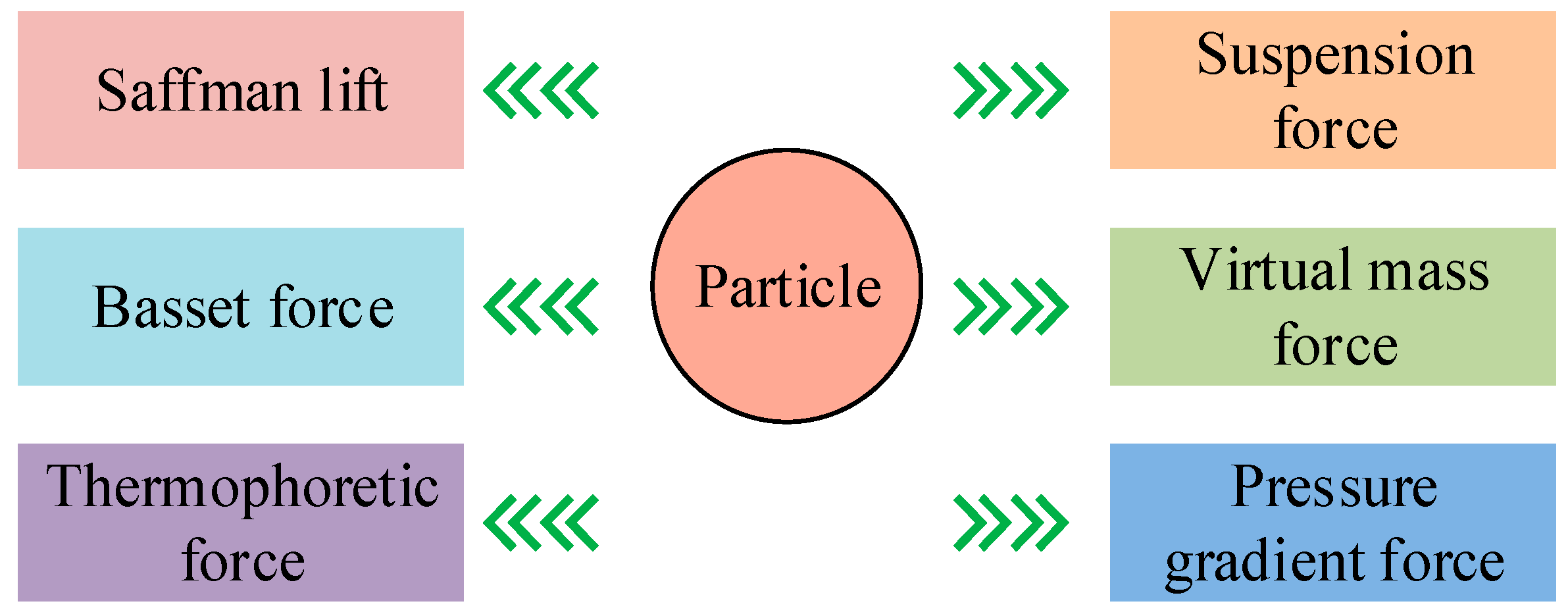
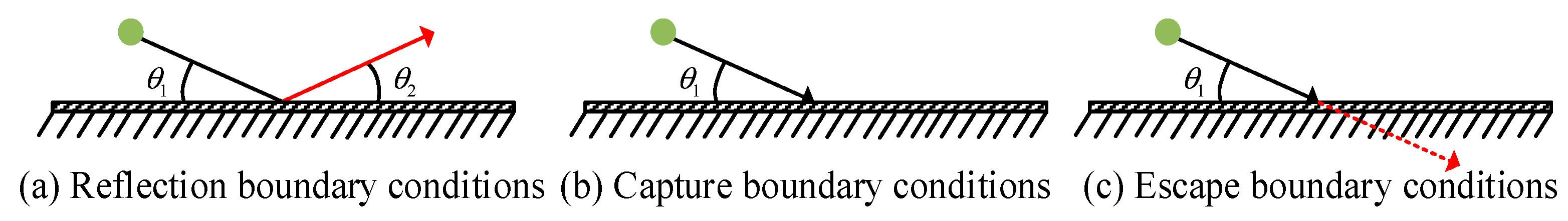
2.1. Construction of Numerical Models for Airflow Organization and Aerosol Diffusion

To find the safest and most comfortable indoor ventilation method, numerical simulation methods were used to construct numerical models for airflow organization and aerosol diffusion. Based on the indoor airflow organization and aerosol diffusion under different ventilation methods, the study selected the indoor ventilation technologies that need to be optimized in the future. Four indoor ventilation methods were selected for the study, namely mixed ventilation, “air rain” flow field, floor air supply, and displacement ventilation. To simulate different ventilation methods, Computational Fluid Dynamics (CFD) simulations were utilized in the study. CFD simulation can eliminate the influence of uncontrollable factors, simulate multiple situations in a short time, and parameter modification is also very convenient [16]. For the basic control equation of continuous phase, the Boussinesq hypothesis was adopted to handle the buoyancy caused by temperature difference in the study. The general expression of the continuous phase control equation is shown in Equation (1) [17].
S Φ = ρ g Φ t + × ( ρ g Φ U g Γ Φ grad Φ )
In Equation (1), Φ represents the general variable, represents the Hamiltonian operator, Γ Φ means the generalized diffusion coefficient, S Φ refers to the generalized source term, ρ means fluid density, t represents time, U g represents gas composition, g is the gravitational acceleration, is the calculation of partial derivatives, ρ g is the gravity density, and grad is the percentage system. The flow characteristics of indoor air are turbulent flow. To numerically simulate turbulent flow, the Reynolds averaging method, which is a non-direct numerical simulation method, was used in the study. The k-ε and k-ω models in the Reynolds-averaged eddy viscosity model are common turbulence models [18]. To better simulate turbulent flow, the study adopted the k-ε shear stress model that combines the advantages of k-ε and k-ω models. The convective diffusion process of microbial particles in indoor flow fields can be regarded as a gas–solid two-phase flow. To solve the two-phase flow problem, the study adopted the particle tracking method for numerical simulation, which is a discrete dispersed particle model. The motion trajectory equation of a single particle is shown in Equation (2).
d u W d t = F D ( u u W ) + g ( ρ W ρ ) ρ W + F i
In Equation (2), F D ( u u W ) represents the fluid drag force acting on the particles, g ( ρ W ρ ) ρ W represents the gravity and buoyancy acting on the particles, F i represents the additional force acting on the particles, u W represents the speed of particle movement, u refers to the speed of airflow movement, ρ W is the densities of particles, and W represents particles, d t represents differential operation, and d is the symbol of differential operation. The additional force acting on the particles is shown in Figure 1.
From Figure 1, it can be seen that the additional forces acting on particles mainly include suspension force, virtual mass force, pressure gradient force, thermal swimming force, Saffman lift, and Basset force. The calculation of suspension force is shown in Equation (3) [19].
F B = π 6 d W 3 ( ρ W ρ ) g
In Equation (3), d represents the particle diameter (simplified as a sphere), and F B represents suspension force. The model needs to incorporate mixed discrete phase boundary conditions, including reflection boundary conditions, capture boundary conditions, escape boundary conditions, wall jet boundary conditions, wall thin-film boundary conditions, and user-defined boundary conditions. Among them, reflection, capture, and escape boundary conditions are the most important, as shown in Figure 2.
In Figure 2, θ 1 and θ 2 represent the angles of incidence and reflection, respectively. Figure 2a–c illustrate the boundary conditions for particle reflection, capture, and escape, respectively. For reflection boundary conditions, it is mainly necessary to consider the energy loss caused by non-elastic collision with the wall. When the trajectory calculation is terminated, particles are recorded as “captured”. When a particle encounters an escape boundary, it will “escape”, and trajectory calculation will also stop. The schematic diagram of the numerical calculation physical model is denoted in Figure 3.
From Figure 3, it can be seen that the length, width, and height of the numerical calculation physical model are 3.5 m, 2.4 m, and 3 m, respectively. The distance between two human models is 0.5 m, and one person is the source of infection, while the other person is a susceptible person. On the body surface, room floor, ceiling, and tabletop, capture boundary conditions are used in the study, while on the human mouth, air supply outlet, and exhaust outlet, escape boundary conditions are used in the study.

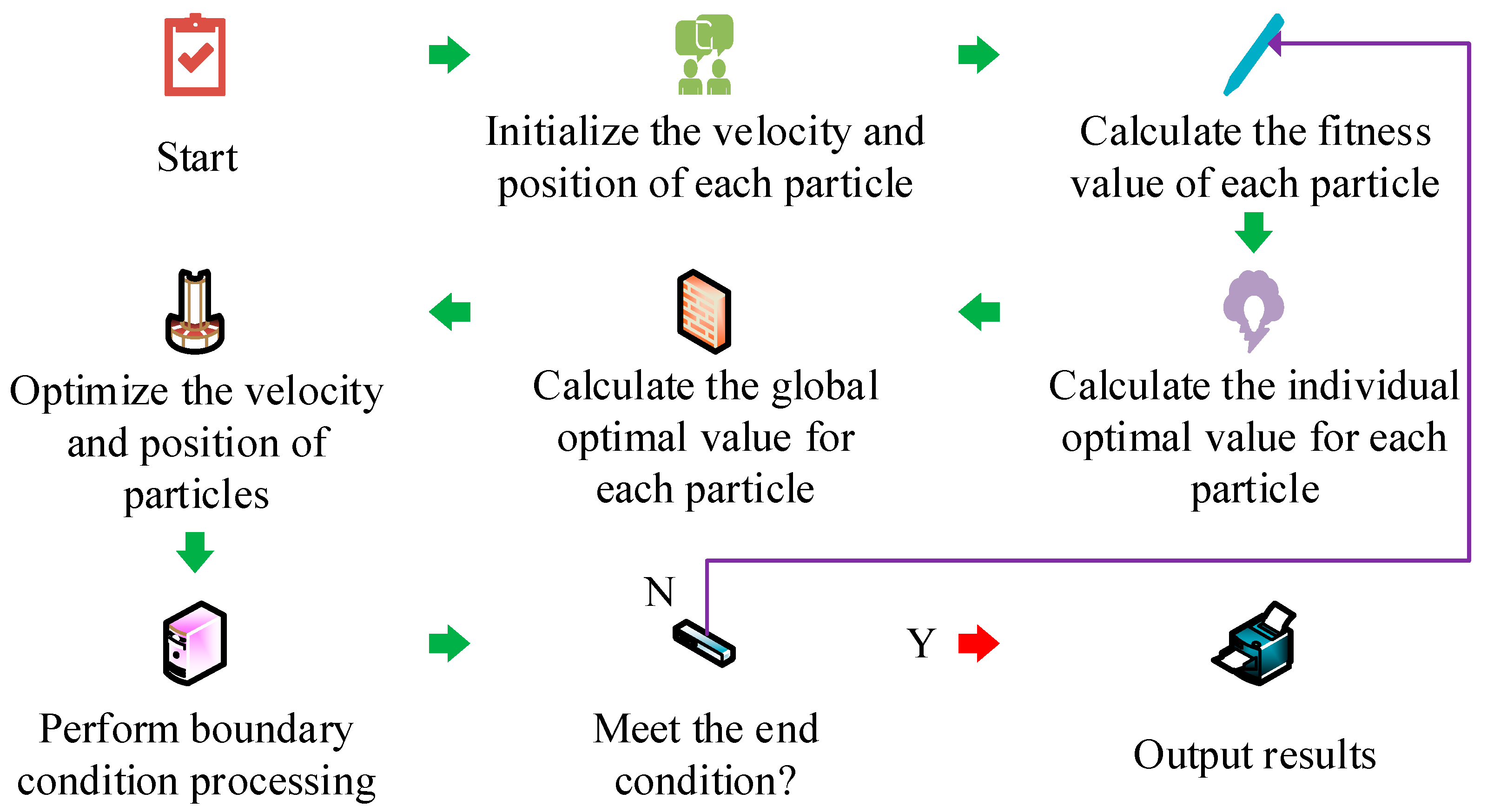
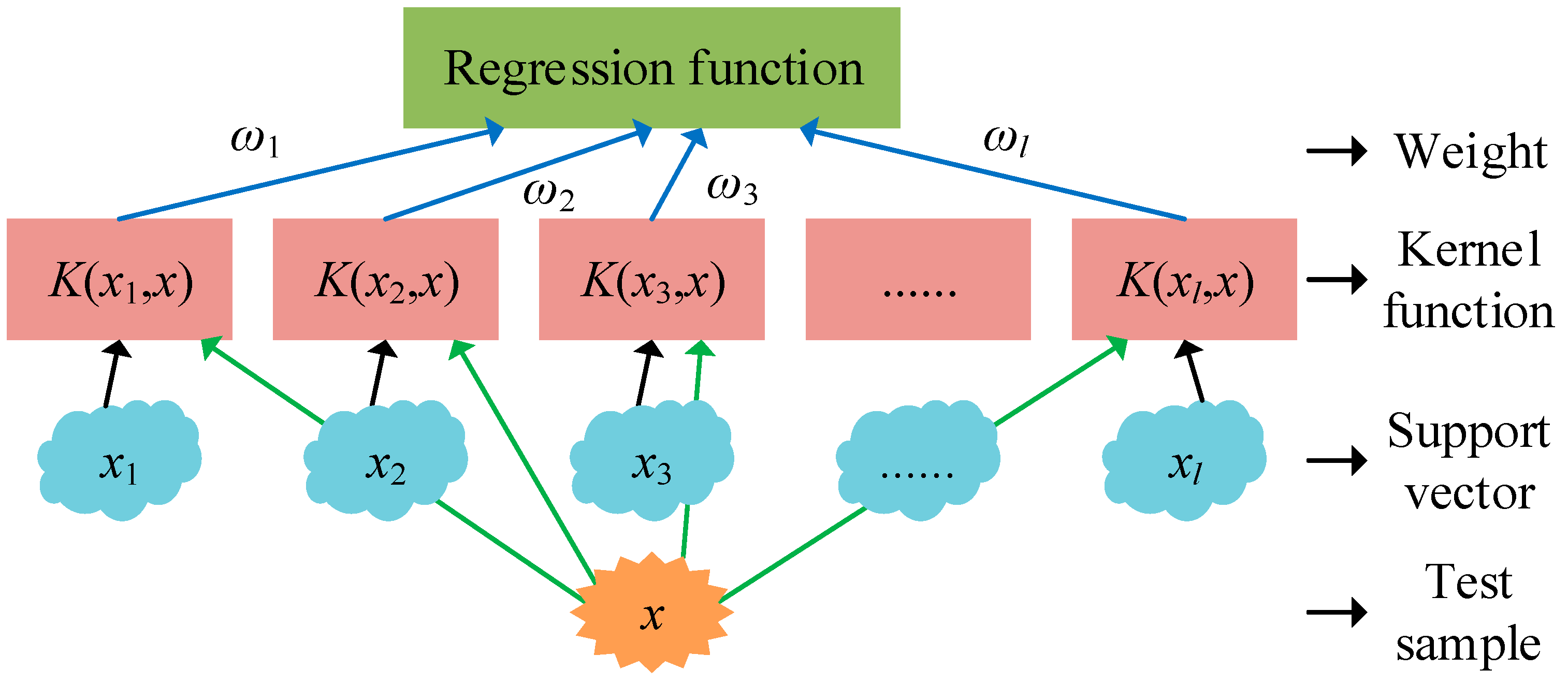
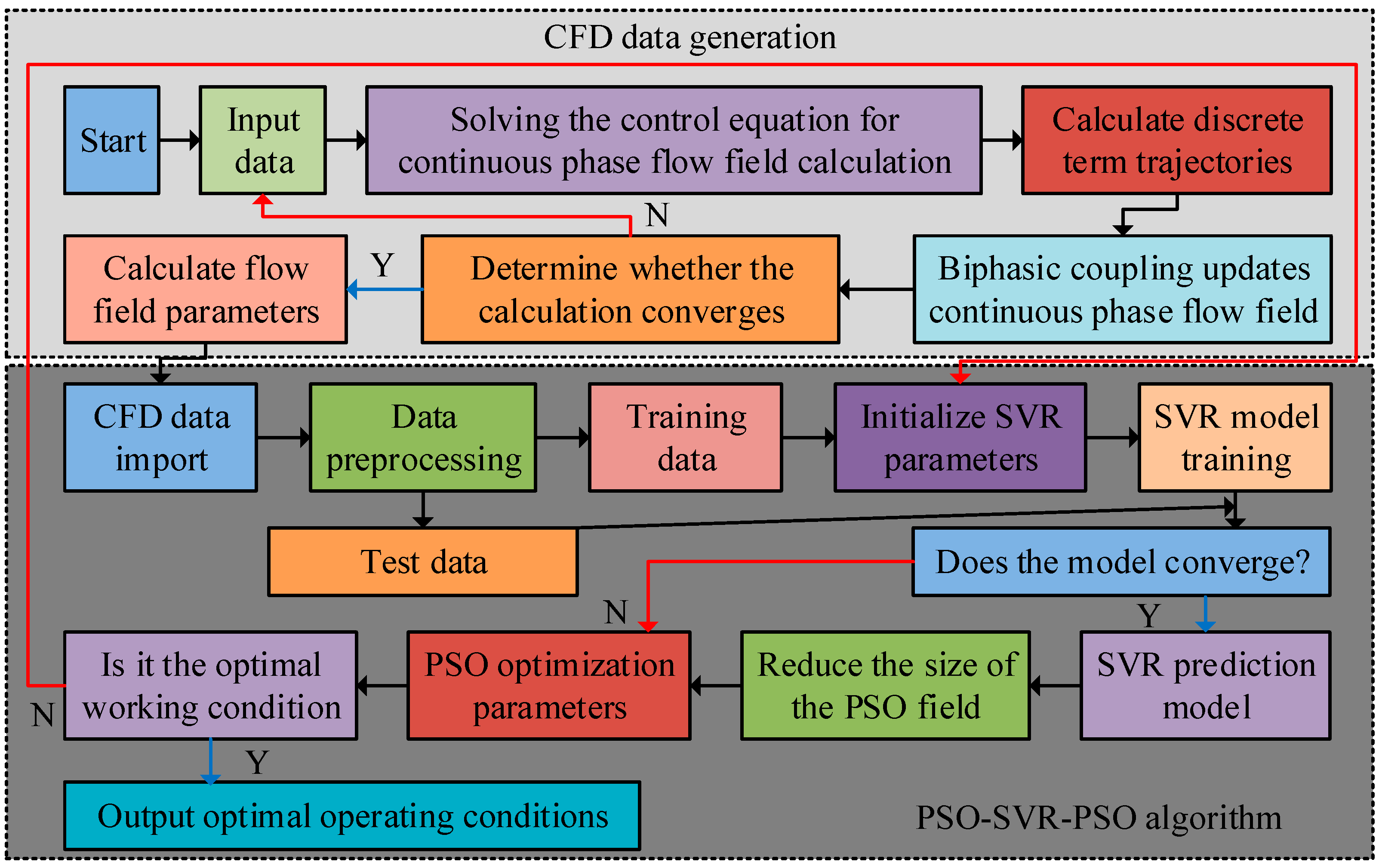
2.2. Design of Improved SVR-PSO Algorithm for Multi-Objective Optimization of Ventilation Methods

To simulate the airflow organization and aerosol diffusion inside the building, a corresponding numerical model was constructed. Based on this numerical model, the thermal comfort and aerosol propagation under different air supply methods were simulated. Based on the simulation results, the study selected a more advantageous “air rain” flow field for further optimization. The specific simulation results will be developed later. The “air rain” flow field can suppress the diffusion of indoor pollutants, but there are also some shortcomings, such as the need for suspended floors and suspended ceilings throughout the house. However, suspended flooring is costly and difficult to clean [20]. Therefore, the study will conduct multi-objective optimization from the positions of the return air and inlet air. With the development of artificial intelligence, more and more algorithms are being developed to solve real-world problems. PSO has the advantages of simplicity, high accuracy, and fast convergence, and has good advantages in solving practical problems. The main process of the PSO algorithm is shown in Figure 4 [21].
From Figure 4, the first step of the PSO algorithm process is to initialize the velocity and position of each particle, and the second step is to calculate the fitness value of each particle. The third step is to calculate the individual optimal value for each particle, and the fourth step is to calculate the global optimal value for each particle. The fifth step is to optimize the velocity and position of particles, and the sixth step is to perform boundary condition processing. The seventh step is to determine whether the constraint conditions are met. If it is determined to be yes, the output result ends the process. Otherwise, it returns to the third step. However, the PSO algorithm is prone to falling into local optima, so research will optimize it. SVR is an important branch of Support Vector Machine, which can greatly reduce computational cost [22]. Therefore, the study will use SVR to optimize PSO and form the SVR-PSO algorithm. The main process of SVR is shown in Figure 5.
From Figure 5, the main process of SVR involves regression functions, weights, kernel functions, support vectors, and test samples. Among them, x 1 , x 2 , , x l is the input, ω 1 , ω 2 , , ω l is the weight, l represents the serial number, and x is the test sample. K ( x l , x ) represents the total number of serial numbers. The kernel function used in the study is Gaussian kernel function. The expression of the regression function is shown in Equation (4).
f ( x ) = ω x + b
In Equation (4), b represents the threshold. The method of seeking the lowest regression risk in SVR is shown in Equation (5).
min ω , b , ζ , ζ 1 2 ω T ω + C L = 1 l ( ζ L + ζ L )
In Equation (5), ζ L represents the upper limit training error, and ζ L represents the lower limit training error. C is the regularization penalty term, and L is the L -th. ω T represents the transpose of weights. To minimize the regression risk in SVR, constraints need to be met, as shown in Equation (6).
s . t . { y L ( ω , x + b ) ε + ζ L ( ω , x + b ) y L ε + ζ L ζ L , ζ L 0
In Equation (6), ε represents the insensitive loss function, and y L is the second input in the kernel function. The general expression of kernel function is shown in Equation (7).
K ( x , y ) = exp ( σ x y 2 )
In Equation (7), σ represents the kernel parameter of the kernel function, and x and y are both input variables of the kernel function. The final regression function is shown in Equation (8).
f ( x ) = L = l l ( a L a L ) K ( x L , x j ) + b
In Equation (8), a L and a L are both Lagrangian coefficients, and their values are ≥ 0. K ( x L , x j ) is the kernel function. x L and x j are the input values in the kernel function, where j is the ordinal. To better leverage the performance of the SVR-PSO algorithm, research optimized it to form the final PSO-SVR-PSO algorithm. The specific optimization approach is to first use the SVR-PSO algorithm to construct a predictive model for CFD data, followed by PSO iterative calculation to perform multi-objective optimization on the ventilation mode. The optimization process of the PSO-SVR-PSO algorithm is denoted in Figure 6.
From Figure 6, the optimization of the PSO-SVR-PSO algorithm is mainly divided into two parts. The first part is CFD data generation, and the second part is the specific process of the algorithm. The first step in generating CFD data is to input the data, and the second step is to solve the control equation for the continuous phase flow field calculation. The third step is to calculate the trajectory of the discrete term, and the fourth step is to update the continuous phase flow field through two-phase coupling. The fifth step is to determine whether the calculation converges. If it converges, it will calculate the flow field parameters. Otherwise, it will go back to the first step. The first step in the specific process of the PSO-SVR-PSO algorithm is to import CFD data, and the second step is to preprocess the data. The third step is to divide the data into training data and testing data. The fourth step is to initialize the SVR parameters. The fifth step is to train the SVR model, and the sixth step is to combine test data to determine whether the model converges. If convergence occurs, it will output the SVR prediction model, then reduce the size of the PSO domain and optimize the parameters for PSO. Otherwise, PSO optimization parameters will be directly carried out. The seventh step is to determine whether it is the optimal working condition. If it is determined to be the optimal working condition, it will output the optimal working condition. Otherwise, it will go back to the fourth step. For the multi-constraint optimization of ventilation methods, the evaluation criteria used in the study involve infection probability, thermal comfort, energy utilization coefficient, and velocity non-uniformity coefficient. Heat comfort measures used the Predicted Mean Vote and Predicted Percentage Dissatisfied (PMV-PPD) indicators. The solution of Predicted Mean Vote P M V is shown in Equation (9).
P M V = [ 0.303 exp ( 0.036 M ) + 0.028 ] ψ
In Equation (9), M represents the metabolic rate of the human body, and ψ represents the abbreviation of the formula. The specific expansion of ψ is shown in Equation (10).
ψ = M { 3.96 × 10 8 f C η [ ( T C η + 273.15 ) 4 ( T r + 273.15 ) 4 ] + f C η h C ( T C η T ) + 3.05 × 10 3 [ 5733 6.99 ( M ) Q α ] + 0.42 ( M 58.15 ) + 1.7 × 10 5 M ( 58667 Q α ) + 0.0014 M ( 34 T ) }
In Equation (10), denotes the mechanical work performed by the human body, and f C η represents the correlation between the surface coverage area coefficient of the human body and the thermal resistance of the clothing. T C η denotes the surface temperature of human clothing, while T r represents the average radiation temperature. h C denotes the surface heat transfer coefficient between indoor air and human clothing, and T represents the air temperature within the range of human activity. Q α is the partial pressure of water vapor in the vicinity of the human body. C represents human clothing, and C η represents the appearance of human clothing. The calculation of f C η is shown in Equation (11).
f C η = { 1.29 I C η + 1 , i f I C η < 0.078 0.645 I C η + 1.05 , o t h e r w i s e I C η 0.078
In Equation (11), I C η represents the thermal resistance of human clothing. The calculation of T C η is shown in Equation (12).
T C η = 35.7 0.028 ( M ψ ) I C η { 3.96 × 10 8 f C η [ ( T C η + 273.15 ) 4 ( T r + 273.15 ) 4 ] + f C η h C ( T C η T ) }
In addition, the calculation of h C is shown in Equation (13).
h C = { 12.1 u ¯ 0.5 , i f 2.38 ( T C η T ) 0.25 < 12.1 u ¯ 0.5 2.38 ( T C η T ) 0.25 , o t h e r w i s e 2.38 ( T C η T ) 0.25 12.1 u ¯ 0.5
In Equation (13), u ¯ represents the indoor airflow velocity. The calculation of energy utilization coefficient is shown in Equation (14).
= H β H s H n H s
In Equation (14), H β represents the exhaust temperature, H n represents the average temperature of the indoor human activity area, and H s represents the supply air temperature. The study normalized and weighted four different evaluation criteria. The expression of the multi-constraint optimization mathematical model E of the PSO-SVR-PSO algorithm is shown in Equation (15).
E = 0.3 × | F 1 | + 0.3 × F 2 0.25 × F 3 + 0.15 × F 4
In Equation (15), F 1 , F 2 , F 3 , and F 4 represent the objective functions of the thermal comfort index PMV-PPD, infection probability, energy utilization coefficient, and velocity non-uniformity coefficient, respectively.

3. Results and Discussion

To understand the simulation results of different ventilation methods, the effectiveness of the numerical model was verified by comparing the measured and simulated values of the velocity and temperature fields. The ventilation methods were compared from the perspectives of thermal comfort and aerosol particle fate to determine the optimal ventilation method. In addition, the performance of the PSO-SVR-PSO algorithm was also validated through research, with validation indicators including PMV, infection probability, non-uniformity coefficient, energy utilization coefficient, and fitting optimization results.

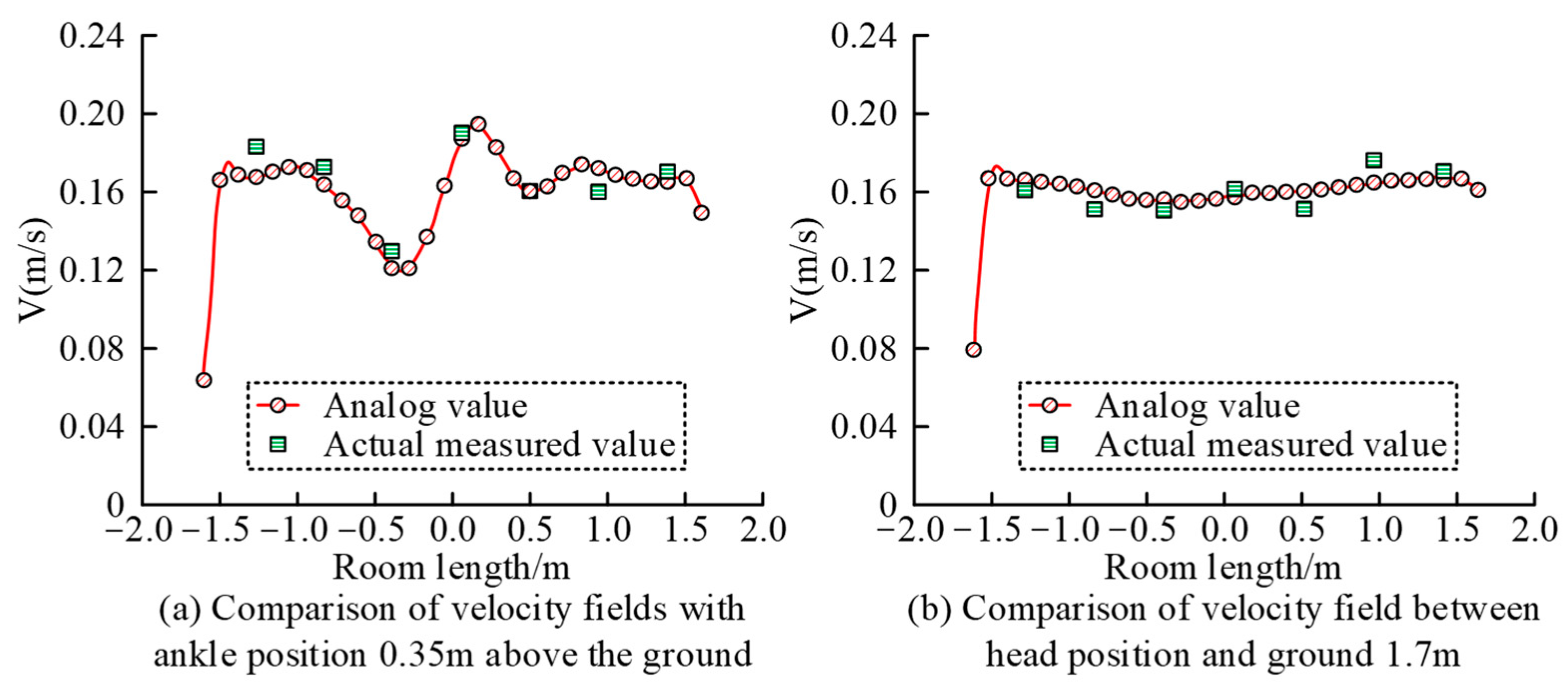
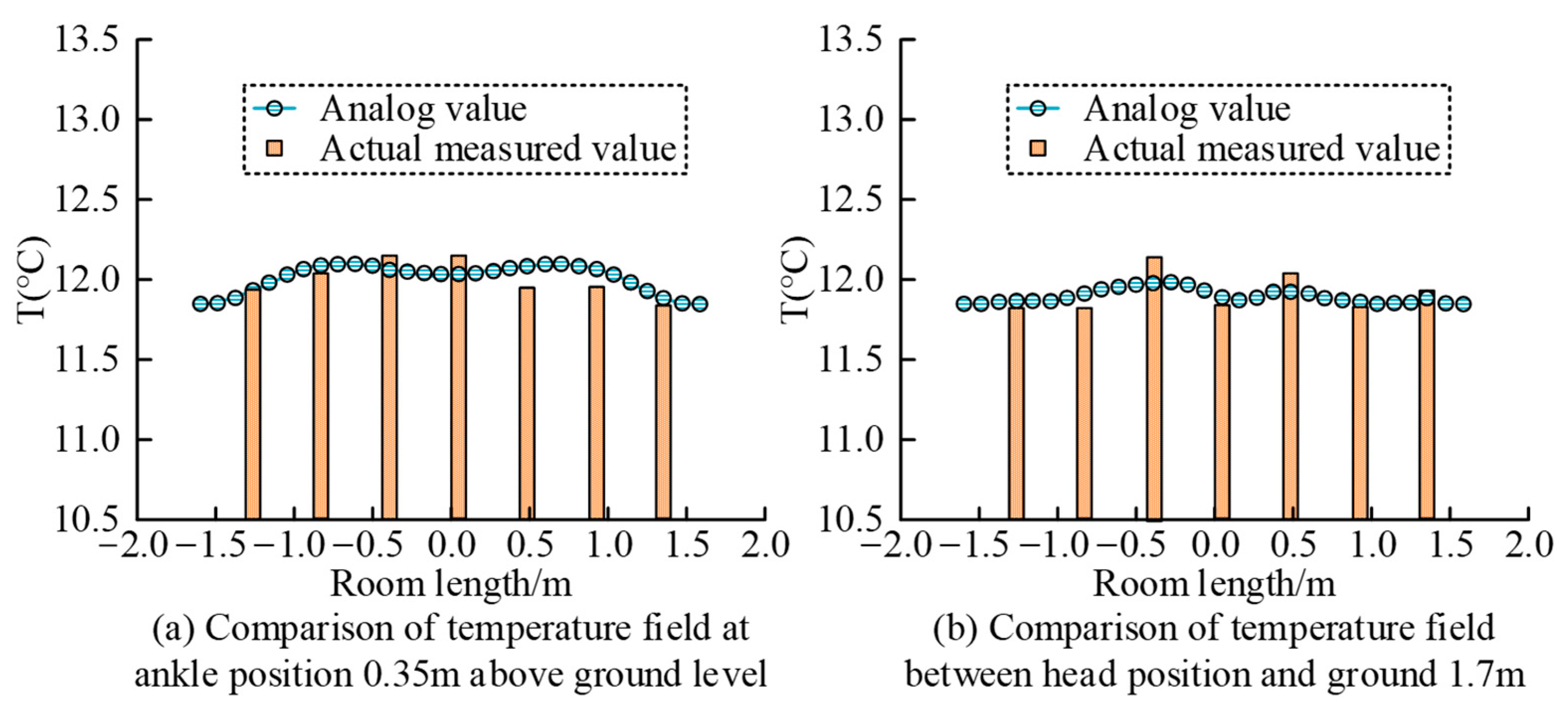
3.1. Validation of Numerical Models

To verify the effectiveness of the numerical model constructed by the research institute, an experimental chamber consistent with the numerical model was constructed. The length, width, and height of the experimental module were consistent with the numerical model, which were 3.5 m, 2.4 m, and 3 m, respectively. In addition, the experimental module involved dummy modes, lower air duct interlayers, upper air duct interlayers, exhaust ducts, porous ceilings, floor holes, and high-efficiency particulate air filters. The experimental cabin simulated two ventilation scenarios, namely the “air rain” flow field and mixed ventilation. The data collection in the experimental cabin was mainly achieved using temperature transmitters and miniature wind speed transmitters. The tracer bacteria used in the experiment was the Escherichia coli FSCC149002 strain, and the colorimetric medium was Escherichia coli, a microbial species. The operating system used in the experiment was Windows 11, the processor was Intel Core i5-12600K, the maximum RF frequency was 4.90 GHz, and the maximum memory was 128 GB. The comparison between the measured and simulated values of velocity fields at different positions is shown in Figure 7.
According to Figure 7a, when the ankle position was 0.35 m away from the ground, the measured velocity fields at seven experimental points were 0.181 m/s, 0.172 m/s, 0.128 m/s, 0.186 m/s, 0.158 m/s, 0.158 m/s, and 0.170 m/s, respectively. The corresponding simulated values were 0.168 m/s, 0.162 m/s, 0.120 m/s, 0.184 m/s, 0.158 m/s, 0.173 m/s, and 0.168 m/s. The measured and simulated values of the velocity field were very close. From Figure 7b, when the head position was 1.7 m away from the ground, the measured velocity fields at the seven experimental points were 0.160 m/s, 0.150 m/s, 0.151 m/s, 0.161 m/s, 0.150 m/s, 0.175 m/s, and 0.165 m/s, respectively. The corresponding simulated values were 0.162 m/s, 0.159 m/s, 0.157 m/s, 0.158 m/s, 0.159 m/s, 0.162 m/s, and 0.164 m/s. The measured and simulated values of the velocity field were also very close at this time, indicating that the numerical model constructed by the research institute was effective. The comparison between the measured and simulated values of temperature fields at different positions is shown in Figure 8.
From Figure 8a, when the ankle position was 0.35 m away from the ground, the measured temperature fields at seven experimental points were 11.90 °C, 12.00 °C, 12.10 °C, 12.10 °C, 11.90 °C, 11.90 °C, and 11.80 °C, respectively. The corresponding simulated values were 11.92 °C, 12.08 °C, 12.06 °C, 12.02 °C, 12.08 °C, 12.04 °C, and 11.89 °C. The difference between the measured value and the simulated value was less than 0.2, and the difference was very small. According to Figure 8b, when the head position was 1.7 m away from the ground, the measured temperature fields at seven experimental points were 11.80 °C, 11.80 °C, 12.10 °C, 11.80 °C, 12.00 °C, 11.80 °C, and 11.90 °C, respectively. The corresponding simulated values were 11.85 °C, 11.90 °C, 11.98 °C, 11.87 °C, 11.93 °C, 11.85 °C, and 11.85 °C, respectively. The difference between the measured value and the simulated value was also less than 0.2, and the difference was also very small. From this, it can be seen that the numerical model constructed by the research institute is effective.

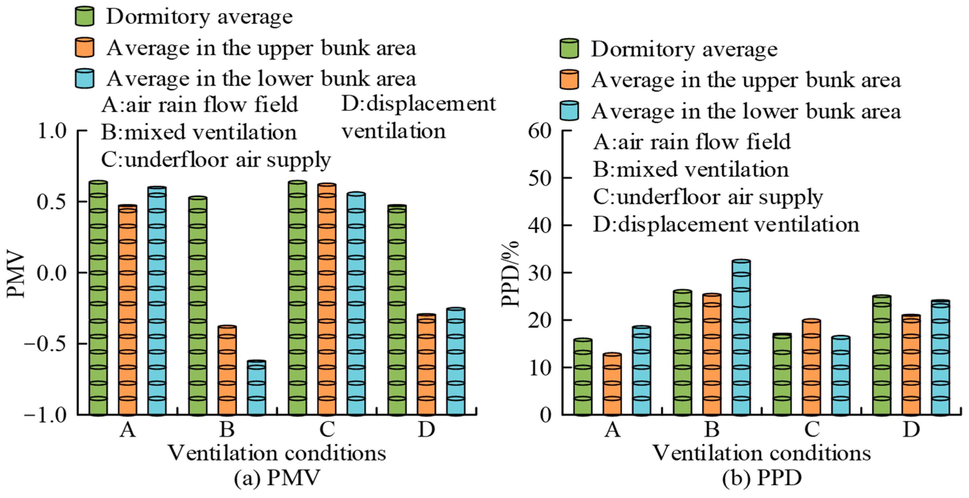
3.2. Simulation Results Analysis of Different Ventilation Methods

To determine the optimal ventilation method, a comparative analysis was conducted on the thermal comfort and aerosol particle fate under different ventilation methods. In the simulation experiment, the temperature of the velocity inlet was set to 300 K, and the flow field of “air rain” and the floor air supply velocity were set to 0.15 m/s. Based on the same air supply volume, the mixed ventilation and displacement ventilation velocities were calculated to be 3.78 m/s. The comparison of thermal comfort between different ventilation methods is shown in Figure 9.
According to Figure 9a, the average indoor value of the “air rain” flow field was 0.63 on the PMV value, and the average values of the upper and lower indoor areas were 0.49 and 0.58, respectively. The average PMV values for indoor, upper, and lower bunk areas with mixed ventilation were −0.52, −0.36, and −0.59, respectively. The average PMV values for indoor, upper, and lower bunk areas with underfloor ventilation were 0.63, 0.61, and 0.56, respectively. The average PMV values for indoor, upper, and lower bunk areas with displacement ventilation were −0.49, −0.32, and −0.27, respectively. From Figure 9b, the average values of the indoor, upper, and lower areas of the “air rain” flow field on the PPD value were 16.14, 12.89, and 19.38, respectively. The average PPD values for indoor, upper, and lower bunk areas with mixed ventilation were 27.58, 27.53, and 32.85, respectively. The average PPD values for indoor, upper, and lower bunk areas with underfloor ventilation were 17.73, 18.18, and 16.86, respectively. The average PPD values for indoor, upper, and lower bunk areas with displacement ventilation were 25.87, 21.25, and 24.40, respectively. A PMV of 0 was the most suitable state for the human body to be indoors, while the PPD index should be less than 26%. From this, the dissatisfaction rate with the thermal comfort of the “air rain” flow field and floor air supply is lower. The comparison of aerosol particle fate under different ventilation methods is shown in Figure 10.
From Figure 10a, under the “air rain” flow field, the maximum number of aerosol particles that the human body comes into contact with was 171, and the minimum number was 4. The maximum number of aerosol particles in contact with the bed surface was 769, and the minimum number was 169. The maximum value of aerosol particles at the outlet was 19,973, and the minimum value was 2197. Most aerosol particles have escaped from the exit, posing a relatively small threat to indoor personnel. According to Figure 10b, under mixed ventilation, the maximum and minimum values of aerosol particles in contact with the human body, bed surface, and outlet were 2559 and 599, 1967 and 298, and 16,733 and 769, respectively. According to Figure 10c, under floor air supply, the maximum and minimum values of aerosol particles in contact with the human body, bed surface, and outlet were 295 and 46, 1973 and 294, and 18,885 and 15,394, respectively. From Figure 10d, under displacement ventilation, the maximum and minimum values of aerosol particles in contact with the human body, bed surface, and outlet were 2699 and 259, 4653 and 1721, and 13,243 and 2893, respectively. From this, under the “air rain” flow field, the human body and the bed come into contact with the least amount of aerosol particles, so the “air rain” flow field is a better ventilation method.

3.3. Analysis of Multi-Objective Optimization Results for the “Air Rain” Flow Field

To verify the performance of the PSO-SVR-PSO algorithm, 256 sets of data were selected for the study, which were provided by CFD simulation. The initial dataset involved PMV, infection probability, non-uniformity coefficient, and energy utilization coefficient. Seventy percent of the data in the dataset was used for training, and the remaining data were used for prediction. The comparison of fitting optimization before and after algorithm optimization is shown in Figure 11.
According to Figure 11a, before optimizing the algorithm, the max value of the original non-uniformity coefficient was 0.44, and the mini value was 0.08. The max value of the non-uniformity coefficient predicted by the PSO algorithm was 0.36, and the mini value was 0.18. The difference between the predicted values of the PSO algorithm and the original values was significant. As shown in Figure 11b, after optimizing the algorithm, the max predicted non-uniformity coefficient by the PSO-SVR-PSO algorithm was 0.457, and the mini value was 0.08. The predicted values of the PSO-SVR-PSO algorithm were very close to the original values. The comparison of PMV, infection probability, non-uniformity coefficient, and energy utilization coefficient before and after working condition optimization is shown in Figure 12.
From Figure 12a, the mean values of the original data on PMV values were 0.397, 0.366, 0.429, 0.349, 0.326, 0.344, 0.416, and 0.452, respectively. The mean values of the data after multi-objective optimization using the PSO-SVR-PSO algorithm were 0.187, 0.236, 0.192, 0.216, 0.194, 0.185, 0.198, and 0.319, respectively. The original mean and optimized mean of the non-uniformity coefficient were 0.268 and 0.152, respectively. After optimizing the working conditions, the overall indoor thermal comfort was improved to a certain extent, and the indoor gas distribution was more uniform. In Figure 12b, in terms of infection probability, the mean values of the original data were 0.0036%, 13.9919%, 0.8749%, 0.0049%, 0.0024%, and 14.3899%, respectively. The mean values of the data after multi-objective optimization using the PSO-SVR-PSO algorithm were 0%, 1.9681%, 0%, 0%, 0%, and 0.1316%, respectively. The original mean and optimized mean of energy utilization coefficient were 0.95 and 1.38, respectively. After optimizing the working conditions, the indoor infection rate and energy consumption of the ventilation system were significantly reduced.

4. Conclusions

To optimize the ventilation method inside the building, a numerical model of airflow organization and aerosol diffusion was studied and constructed to determine the optimal ventilation method, and the PSO-SVR-PSO algorithm was designed. The results showed that the measured and simulated values of velocity and temperature fields were very close at different positions, indicating that the numerical model constructed in the study was effective. The average PMV values of the “air rain” flow field in the indoor, upper, and lower bunk areas were 0.63, 0.49, and 0.58, respectively, and the PPD values were 16.14, 12.89, and 19.38, respectively. In addition, under the “air rain” flow field, the maximum values of aerosol particles at the human body, bed surface, and outlet were 171, 769, and 19,973, respectively, and the minimum values were 4, 169, and 2197, respectively. The “air rain” flow field was the optimal ventilation method. The maximum and minimum values of the original non-uniformity coefficient were 0.44 and 0.08, respectively. The PSO-SVR-PSO algorithm predicted a maximum non-uniformity coefficient of 0.457 and a minimum coefficient of 0.08. The original value and predicted value were very close. In addition, in terms of infection probability, the mean values of the data after multi-objective optimization using the PSO-SVR-PSO algorithm were 0%, 1.9681%, 0%, 0%, 0%, and 0.1316%, respectively. The PSO-SVR-PSO algorithm had good performance. However, in daily life, a ventilation mode cannot be well applied to all indoor environments, an aspect which is also lacking in research. Future research can quantitatively evaluate the feasibility of various ventilation methods in different scenarios.

Author Contributions

Conceptualization, M.H. and C.K.; methodology, M.H.; software, S.Y.; validation, M.H., C.Z. and J.J.; formal analysis, C.Z. and S.Y.; investigation, C.Z.; resources, C.K.; data curation, C.Z.; writing—original draft preparation, M.H.; writing—review and editing, C.K.; visualization, J.J.; supervision, C.Z.; project administration, C.K.; funding acquisition, C.K. All authors have read and agreed to the published version of the manuscript.

Funding

This work was supported by a grant from the Brain Korea 21 Program for Leading Universities and Students (BK21 FOUR) MADEC Marine Design Engineering Education Research Group.

Institutional Review Board Statement

Not applicable.

Informed Consent Statement

Not applicable.

Data Availability Statement

Data is contained within the article.

Conflicts of Interest

The authors declare no conflicts of interest.

References

  1. Nazaroff, W.W. Indoor particle dynamics. Indoor Air 2004, 14, 175–183. [Google Scholar] [CrossRef] [PubMed]
  2. Loth, E. Numerical approaches for motion of dispersed particles, droplets and bubbles. Prog. Energy Combust. Sci. 2000, 26, 161–223. [Google Scholar] [CrossRef]
  3. Dhahri, M.; Aouinet, H. Investigation of temperature distribution, air flow pattern and thermal comfort in natural ventilation of building using solar chimney. World J. Eng. 2020, 17, 78–86. [Google Scholar] [CrossRef]
  4. Xie, E.; Zhao, W.; Xu, Z.; Zhang, X.; Xu, W.; Wang, T. A numerical study on smoke back-layering length in V-shaped tunnels under natural ventilation. Fire Mater. 2022, 46, 130–143. [Google Scholar] [CrossRef]
  5. Degois, J.; Veillette, M.; Poulin, P.; Lévesque, B.; Duchaine, C. Indoor air quality assessment in dwellings with different ventilation strategies in Nunavik and impacts on bacterial and fungal microbiota. Indoor Air 2021, 31, 2213–2225. [Google Scholar] [CrossRef] [PubMed]
  6. Wang, J.; Jia, M.; Bin, L.; Wang, L.; Zhong, D. Regulation and optimization of air quantity in a mine ventilation network with multiple fans. Arch. Min. Sci. 2022, 67, 179–193. [Google Scholar]
  7. Song, C.; Zhao, T.; Liu, Y.; Wang, D. Distribution characteristics of indoor oxygen concentration under natural ventilation in oxygen-enriched buildings at high altitudes. Build. Simul. 2021, 14, 1823–1841. [Google Scholar] [CrossRef]
  8. Jeong, S.G.; Wallace, L.; Rim, D. Contributions of Coagulation, Deposition, and Ventilation to the Removal of Airborne Nanoparticles in Indoor Environments. Environ. Sci. Technol. 2021, 55, 9730–9739. [Google Scholar] [CrossRef] [PubMed]
  9. Ghazvineh, S.; Salimi, M.; Dehghan, S.; Asemi-Rad, A.; Dehdar, K.; Salimi, A. Stimulating olfactory epithelium mitigates mechanical ventilation-induced hippocampal inflammation and apoptosis. Hippocampus 2023, 33, 880–885. [Google Scholar] [CrossRef]
  10. Lee, J.A.; Mcpeck, M.; Cuccia, A.D.; Smaldone, G.C. Real-Time Analysis of Dry-Side Nebulization with Heated Wire Humidification During Mechanical Ventilation. Respir. Care 2022, 67, 914–928. [Google Scholar] [CrossRef]
  11. Ting, C.H.; Tan, F.W.; Kuo, C.L. Investigations of structure strength and ventilation performance for agriproduct corrugated cartons under long-term transportation trip. Packag. Technol. Sci. 2022, 35, 821–832. [Google Scholar]
  12. Wang, S.; Xing, J.; Jiang, Z.; Dai, Y. A decentralized, model-free, global optimization method for energy saving in heating, ventilation and air conditioning systems. Build. Serv. Eng. Res. Technol. 2020, 41, 414–428. [Google Scholar] [CrossRef]
  13. Ju, F.L.; Liu, L.; Yu, X. An analytical study to evaluate the impact of distributed zone fans on the air flow rate in a mechanical ventilation system. Build. Serv. Eng. Res. Technol. 2020, 41, 507–516. [Google Scholar] [CrossRef]
  14. Singh, M.; Jradi, M.; Shaker, H.R. Monitoring and Evaluation of Building Ventilation System Fans Operation using Performance Curves. Energy Built Environ. 2020, 1, 307–318. [Google Scholar] [CrossRef]
  15. Groumpos, P.P. A Critical Historic Overview of Artificial Intelligence: Issues, Challenges, Opportunities, and Threats. Artif. Intell. Appl. 2023, 1, 197–213. [Google Scholar] [CrossRef]
  16. Olivetti, S.; Gil, M.A.; Sridharan, V.K.; Hein, A.M. Merging computational fluid dynamics and machine learning to reveal animal migration strategies. Methods Ecol. Evol. 2021, 12, 1186–1200. [Google Scholar] [CrossRef]
  17. Cao, Q.; Li, L.; You, H.; Liu, H. Computational study of dynamics of confined droplets under electric field: Effect of contact angle. Int. J. Numer. Methods Heat Fluid Flow 2023, 33, 1775–1796. [Google Scholar] [CrossRef]
  18. Biswas, T.; Dharmatti, S. Interior and H∞ feedback stabilization for sabra shell model of turbulence. Math. Methods Appl. Sci. 2023, 46, 1852–1883. [Google Scholar] [CrossRef]
  19. Kundu, J. Design, analysis, set-up fabrication, control, and a novel analytical approach of a levitation prototype for a symmetric shaped object. Asian J. Control 2023, 25, 537–550. [Google Scholar] [CrossRef]
  20. Liu, D.; Yao, G. Time-varying dynamic analysis of a plate entering the finite subsonic airflow field. Thin-Walled Struct. 2022, 180, 145–157. [Google Scholar] [CrossRef]
  21. Ajmera, K.; Tewari, T.K. SR-PSO: Server residual efficiency-aware particle swarm optimization for dynamic virtual machine scheduling. Extremes 2023, 26, 15459–15495. [Google Scholar] [CrossRef]
  22. Binjie, G.; Jie, C.; Feng, P.; Weili, X. Incremental learning for Lagrangian ε-twin support vector regression. Soft Comput. 2023, 27, 5357–5375. [Google Scholar]
Figure 1. The additional force acting on particles.
Sustainability 16 05256 g001
Figure 2. Specific schematic diagram of reflection, capture, and escape boundary conditions.
Sustainability 16 05256 g002
Figure 3. Schematic diagram of numerical calculation physical model.
Sustainability 16 05256 g003
Figure 4. The main process of the PSO algorithm.
Sustainability 16 05256 g004
Figure 5. The main process of SVR.
Sustainability 16 05256 g005
Figure 6. Optimization process of the PSO-SVR-PSO algorithm.
Sustainability 16 05256 g006
Figure 7. Comparison of measured and simulated values of velocity fields at different positions.
Sustainability 16 05256 g007
Figure 8. Comparison of measured and simulated values of temperature fields at different locations.
Sustainability 16 05256 g008
Figure 9. Comparison of thermal comfort between different ventilation methods.
Sustainability 16 05256 g009
Figure 10. Comparison of the fate of aerosol particles under different ventilation methods.
Sustainability 16 05256 g010
Figure 11. Comparison of fitting optimization before and after algorithm optimization.
Sustainability 16 05256 g011
Figure 12. Comparison of PMV, infection probability, uneven coefficient, and energy utilization coefficient before and after optimization of working conditions.
Sustainability 16 05256 g012
Disclaimer/Publisher’s Note: The statements, opinions and data contained in all publications are solely those of the individual author(s) and contributor(s) and not of MDPI and/or the editor(s). MDPI and/or the editor(s) disclaim responsibility for any injury to people or property resulting from any ideas, methods, instructions or products referred to in the content.

