Improving Order-Picking Performance in E-Commerce Warehouses through Entropy-Based Hierarchical Scattering

Abstract

The high service expectations of e-commerce customers are placing unprecedented demands on e-commerce warehouse workers, leading to higher fatigue and health-related disorders among these workers. Order picking in retail e-commerce fulfilment warehouses (REFWs) is highly labour-intensive and physically demanding activity. This is mainly due to the prevalence of single-unit orders and the expectation of quick order servicing. One strategy to reduce picking effort is the adoption of a scattered storage assignment policy, which spreads the inventory of each product across the entire warehouse. This paper proposes a new, hierarchical approach for the scattering of stock, along with an entropy-based measure for scattering. This measure overcomes some significant limitations of the existing scattering measures and captures the extent of scattering more effectively. We developed a storage assignment heuristic for the scattering of stock and conducted a simulation study to demonstrate its effectiveness in reducing the order-picking effort. Some valuable managerial insights were obtained using a simulation with different warehouse designs and operating parameters. This research also illustrates that the adoption of scattered storage requires careful consideration of the nature of the demand pattern in the warehouse.

1. Introduction

Retail e-commerce sales have grown rapidly in recent years, primarily due to a wide range of product offerings and exceptional customer convenience. By 2027, it is projected that e-commerce will account for approximately one-quarter of the global retail sales [1]. Retail e-commerce fulfilment warehouses (REFWs) play a crucial role in enabling online retailers to meet customer expectations of product availability and servicing time. REFW operations are markedly different from those of traditional warehouses in that they typically store an extremely high range of stock-keeping units (SKUs) and ship a high number of customer orders within a single day [2]. Furthermore, the individual customer orders contain very few line items (e.g., 1.6 items per order for Amazon), with most of the orders having a single unit order per SKU. Also, these orders need to be fulfilled within stringent timelines [2,3].

These characteristics place extreme demands on the order-picking operations of REFWs. Despite recent advances in warehouse automation, most warehouses still use manual, pickers-to-parts process for order picking, where a warehouse picker travels to various storage locations to pick individual items as per a pick list [4]. Manual order picking involves repetitive and physically demanding tasks that makes pickers vulnerable to musculoskeletal disorders (MSDs), including back injuries, sprains, and tears [5,6,7]. It has been established that the cumulative effect of short-term musculoskeletal discomfort amongst warehouse workers leads to long term musculoskeletal pain [8]. A typical e-commerce warehouse picklist consists of many line items, with only one or two units per line item. Unlike in B2B warehouses, where pickers retrieve larger quantities per item, e-commerce pickers spend more time walking to retrieve each item. Although the actual picking time is shorter due to the low quantity per line item, the extensive travel required increases overall fatigue. Furthermore, the strict timelines for fulfilling e-commerce orders add pressure to an already demanding physical task. Consequently, e-commerce warehouses experience a higher incidence of physical injuries than other type of warehouses [9,10]. Minimising worker fatigue and injuries in REFWs is therefore a crucial aspect of research that needs addressing to ensure the sustainable growth in e-commerce. In addition, it is desirable to achieve a uniform distribution of workload across various zones of the warehouse [11].

Most of the time and effort of warehouse pickers is spent in travelling through the warehouse [12]; hence, reducing picking travel is the key to reducing worker fatigue. Picking travel can be influenced through several planning decisions in the warehouse, one of the most critical amongst them being the storage policy of the warehouse [13]. The storage policy of a warehouse determines how the incoming stock is assigned to different storage locations within the warehouse, which in turn affects the distance travelled for order picking.

The storage policies used in traditional warehouses are single-lot storage policies, where the entire inventory of each SKU is stored in a cluster of contiguously located storage locations. These policies are not suitable for e-commerce orders, as they may lead to a high picker travel for a typical REFW picklist with several single unit picks per SKU [14]. Therefore, REFWs have evolved scattered storage policies, where the incoming bulk consignments are broken into put away lots of one or more units and spread over the entire warehouse for storage, [14,15]. Scattered storage offers multiple candidate locations across the entire warehouse for picking each SKU. This stock arrangement enables the picker to complete a picklist comprising many single-item picks within a short travel distance. Hence, maximising the scattering of SKU inventory can reduce the order-picking effort [14]. However, scattered storage assignment requires higher effort in the put away activity. However, the put away activity operates under significantly less time pressure and therefore can be planned at a convenient time to maximise efficiency and reduce stress on workers.

Another critical question in designing a scattered storage policy is how to measure the extent of scattering in a storage assignment. Scattering of stock can be viewed as (a) dispersing the inventory of SKUs across different zones as evenly as possible (geographical dispersion) and (b) assigning storage locations within each zone to the SKUs in a way that maximises the number of uniformly sized clusters (nature of clusters) in the warehouse. Here, a cluster is defined as a set of contiguous storage locations assigned to the same SKU without any intermingling with another SKU. An appropriately defined measure of scattering incorporating these attributes can not only direct the approach used for scattering the stock but also be an appropriate metric for assessing the effectiveness of scattering in reducing the order-picking effort and balancing of load across zones.

Significance of This Research

This is one of the first studies that simultaneously captures several factors related to the scattering of inventory, such as the spread of clusters across many different SKUs, uniformity in cluster sizes, spread of inventory across several zones in the warehouse, and uniformity of the spread of inventory across zones. The existing scattering measures were not employed as objective functions to solve scattered storage assignment problems but used post facto to assess the extent of scattering. In contrast, our research developed an entropy-based metric that quantifies the extent of scattering for a given storage assignment and used the same to solve the scattered storage assignment problem.

The rest of this paper is organised as follows: In Section 2, we review the relevant literature on the scattering of stock, with particular emphasis on the existing measures for scattering and their limitations. In Section 3, we present a new hierarchical approach towards scattering that forms the conceptual foundation of our work. In Section 4, we develop an entropy-based measure for hierarchical scattering that quantifies the extent of scattering. We also demonstrate how the proposed measure overcomes the drawbacks of the existing scattering measures. In Section 5, we formulate an entropy-based storage location assignment problem (ESLAP) that aims to maximise the proposed entropy-based measure. We also present a storage assignment heuristic for solving the ESLAP. In Section 6, we design a simulation study to demonstrate the effect of the proposed scattering approach on warehouse performance under different operating conditions. We present these results in Section 7 and discuss them in Section 8. We conclude this paper in Section 9.

The list of abbreviations used in the text is provided in

Table 1. List of abbreviations used.

REFW	Retail e-commerce fulfilment warehouse
SKU	Stock keeping unit
MSD	Musculoskeletal disorders
ER	Explosion ratio
ESLAP	Entropy-based storage location assignment problem
SSP	Scattered storage policy
SSP(Q)	Scattered storage policy with lot size Q
NLIP	Nonlinear integer program
GA	Genetic algorithm
COL	Closest open location
T/O	Product turnover

.

2. Relevant Literature on Scattered Storage

There is an extensive body of research on traditional storage assignment policies in the warehousing literature [4,13,16,17,18,19,20]. However, scattered storage assignment is a relatively new field of research. Recent research [15,21] has developed various storage assignment methods for scattering inventory in warehouses.

In a pioneering work, Weidinger and Boysen [15] used the concept of ‘measuring points’ spread throughout the warehouse for scattering inventory. They calculated the distance from each measuring point to the nearest item of a SKU and identified the maximum of these distances. Their proposed scattered storage assignment strategy aims to reduce the sum of these maximum distances for all SKUs, thereby spreading the inventory across the warehouse. They showed that such scattering leads to a reduction in picking travel.

Zhang et al. [21] proposed an approach where the incoming inventory of each SKU is split into smaller lots and then allocated to various storage bins to maximise the probability of the completion of picking an order within a short travel distance. Pawar et al. [22] developed a heuristic to show that maximising the entropy of stock arrangement helps with reducing the average aisle spread, which in turn aids with the order-picking process.

Another approach to the storage assignment is affinity-based storage assignment, which focuses on storing the frequently ordered SKUs in close proximity to each other. Such policies can be used in conjunction with a scattering-based approach. Pang and Chan [23] used a data-mining based algorithm for scattered storage assignment, where the correlation between the demand for various SKUs is used to place them in proximity. They showed that their algorithm reduces picking travel compared to the closest open location and dedicated storage policies. Jiang et al. [24] presented an algorithm for storage assignment that minimises the weighted sum of distances between products, with the weights being based on the correlation between the ordering of the products. They solved small-scale problems using genetic-algorithm- and particle-swarm-optimisation-based approaches. For large-scale problems, they proposed a hybrid approach that resulted in significant improvement in picking performance. Krishnamoorthy and Roy [25] adopted high-utility itemset mining to find correlated items instead of using pairwise correlations as well as considered the quantity of each SKU in the orders.

There are only a handful of studies that have attempted to define a numerical measure of scattering. The explosion ratio (ER), proposed by Onal et al. [14], and the warehouse heterogeneity (β), proposed by Weidinger [26], measure the scattering of stock based on the number of clusters of contiguous locations into which the inventory of each SKU is split. Pawar et al. [22] proposed an entropy-based measure (Ey) for the scattering of stock. These measures are explained next.

2.1. Overview of the Existing Scattering Measures

2.1.1. Explosion Ratio (ER) [14]

$$ER=\sum _i{L}_i/\sum _i{V}_i$$

(1)

where

L_i is the number of clusters into which inventory of SKU i is split;

V_i is the total inventory of SKU i.

2.1.2. Warehouse Heterogeneity (β) [26]

$$\beta =\frac{\left(C-I\right)}{(N-I)}$$

(2)

where

C is the total number of clusters into which warehouse inventory is split;

I is the total number of SKUs stored in the warehouse;

N is the total number of storage locations in the warehouse.

2.1.3. Entropy of Stock (Ey) [22]

$$Ey=-\sum _{i=1}^I\sum _{m=1}^M{n}_{im}\mathrm{l}\mathrm{n}\left(n_{im}\right)+\sum _{i=1}^I{N}_i\mathrm{l}\mathrm{n}{(N}_i)$$

(3)

where

$n_{im}$ is the quantity of stock of SKU i stored in zone m;

I is the total number of SKUs stored in the warehouse;

$N_i$ is the total amount of inventory of SKU i;

M is the total number of zones into which the warehouse is divided for the purpose of scattering.

To illustrate these metrics, we consider a warehouse comprising two zones (M = 2), each containing five storage locations (S = 5) (Figure 1). Two SKUs identified as i = A and i = B, having a total inventory of N_A = 6 and N_B = 4 units, are to be stocked in this warehouse. The scattering approach shown in Figure 1 directly splits the given inventory into clusters without considering a possible intermediate step of breaking the inventory into zone-wise quantities.

Here, the clusters for SKUs i = A and i = B are formed, where N_A = 6 is split into three clusters as {4, 1, 1} and N_B = 4 is split as {1, 1, 2} and stored in the two zones. Depending on the number of clusters formed, both across and within the zones, the variables in Equations (1)–(3) can be easily identified for computation of the explosion ratio, the warehouse heterogeneity, and entropy, respectively. Thus, the explosion ratio for the warehouse is calculated using Equation (1):

$$ER=\sum _i{L}_i/\sum _i{V}_i=\frac{3+3}{6+4}=0.6,$$

Warehouse heterogeneity is calculated using Equation (2):

$$\beta =\frac{\left(C-I\right)}{(N-I)}=\frac{6-2}{10-2}=0.5;$$

Entropy is calculated using Equation (3):

$$Ey=-\sum _{i=A,B}\sum _{m=1}^2{n}_{im}\mathrm{l}\mathrm{n}\left(n_{im}\right) + \sum _{i=A,B}{N}_{i}ln {(N}_i)$$

$$Ey=-4\ln \left(4\right)-2\ln \left(2\right)-1\ln \left(1\right)-3\ln \left(3\right)+6\ln \left(6\right)+4 \mathrm{l}\mathrm{n}\left(4\right) = 6.07$$

It is clear from the above calculations that while Equations (1) and (2) use the number of clusters across the whole warehouse, Equation (3) uses the quantity of each SKU within each zone.

2.2. Research Gaps Addressed in This Study

The studies that have attempted to define a numerical measure of scattering are as follows:

(i)

The explosion ratio (ER) was proposed by Onal et al. [14].

(ii)

Warehouse heterogeneity (β), proposed by Weidinger [26], measures the scattering of stock based on the number of clusters of contiguous locations into which the inventory of each SKU is split.

(iii)

Pawar et al. [22] proposed an entropy-based measure (Ey) for the scattering of stock.

Table 2. Comparison of existing scattering measures with the approach developed in this study.

Measure	Aspects of Scattering Considered in the Measure (“√” Indicates Considered, and “-” Indicates Not Considered)
	Nature of Clusters Formed			Geographical Spread of Warehouse Inventory
	Number of Clusters	Spread of Clusters across Many Different SKUs	Uniformity in Cluster Sizes	Spreading Inventory across Several Zones in the Warehouse	Uniformity of Spread of Inventory across Zones
Heterogeneity (β) [26]	√	-	-	-	-
Explosion ratio (ER) [14]	√	-	-	-	-
Entropy (Ey) [22]	-	-	-	√	√
Measure proposed in this study	√	√	√	√	√

compares the above-mentioned scattering measures with the measure proposed in the current study according to their ability to factor in various aspects of scattering.

A good measure of scattering should consider two key aspects. The first one relates to the geographical spread of the inventory of each SKU. The higher the uniformity of the spread, the better the scattering. The second one includes the number and size of the storage clusters formed from the SKU inventory. For effective scattering, it is desirable to have a large number of SKU clusters that are uniform in size and formed across the range of SKUs.

It can be observed from Table 2 that ER and β focus only on the number of clusters formed. They do not control the cluster sizes or their distribution across different SKUs. They also ignore the uniformity in the geographical spread of the clusters. Entropy, Ey, on the other hand, focuses on spreading inventory across the warehouse uniformly and across different SKUs but does not consider the aspect of cluster formation. The measure proposed in this paper aims to capture the two aspects of scattering mentioned above and address the limitations in the cluster formation associated with the existing three measures [14,22,26]. We formulated an entropy-based storage location assignment problem (ESLAP) that aims to maximise the proposed measure. We also developed a heuristic that provides near-optimal solutions to the ESLAP.

3. A New Approach for the Scattering of Stock in a Warehouse

This section introduces our proposed hierarchical approach for scattering and compares it with other approaches.

3.1. Concept of Hierarchical Scattering

We consider a warehouse that is divided into M zones, each containing S storage locations. A zone is defined as a set of contiguous, closely located storage locations. The zone definition can arise out of the warehouse layout, e.g., a single aisle (or multiple adjoining aisles) [22] or a cell of closely located storage locations [21] (Figure 2). Alternatively, we can also divide the warehouse into zones (or sections) of equal storage capacity solely for the purpose of the scattering of stock.

Scattering of stock in a warehouse may manifest at two levels: (1) the distribution of inventory of each SKU across different zones of the warehouse (across-zone scattering) and (2) the formation of SKU clusters within each zone (within-zone scattering).

The following notations serve to introduce these two types of scattering along with the related terminologies:

i is the index variable for a SKU, i $\in$ I_A = {1,2,…I};

m is the index variable for a zone, m $\in$ M_A = {1, 2…M};

s is the index for storage location for each aisle/zone, s $\in$ S_A = {1,2,…S}.

$$Z_{ims }=\left\{\begin{array}{ll}1,& \mathrm{i}\mathrm{f} \mathrm{S}\mathrm{K}\mathrm{U} i \mathrm{i}\mathrm{s} \mathrm{p}\mathrm{l}\mathrm{a}\mathrm{c}\mathrm{e}\mathrm{d} \mathrm{i}\mathrm{n} \mathrm{a}\mathrm{i}\mathrm{s}\mathrm{l}\mathrm{e} m \mathrm{a}\mathrm{n}\mathrm{d} \mathrm{s}\mathrm{t}\mathrm{o}\mathrm{r}\mathrm{a}\mathrm{g}\mathrm{e} \mathrm{l}\mathrm{o}\mathrm{c}\mathrm{a}\mathrm{t}\mathrm{i}\mathrm{o}\mathrm{n} s\\ 0,& \mathrm{o}\mathrm{t}\mathrm{h}\mathrm{e}\mathrm{r}\mathrm{w}\mathrm{i}\mathrm{s}\mathrm{e}\end{array}\right\}$$

K is the size of the picker cart;

N_i is the total amount of inventory of SKU i stored in the warehouse;

N is the total amount of inventory of all SKUs put together, where $N=M\times S$;

R_i is the total units of inventory of SKU i that needs to be assigned to storage locations during replenishment;

R is the total units of inventory in the incoming consignment that need to be assigned to storage locations ${\sum }_{i=1}^{i=I}{R}_i$ = R;

$n_{im}$ is the amount of inventory of SKU i stored in zone m;

${\eta }_{im}^c$ is the amount of inventory of SKU i stored in cluster $c$ in zone m;

$\alpha$ is the heterogeneity of the picklist;

$c$ is the index for a cluster for each SKU i in zone m, $c$ = {1, 2…$,\left|{{\rm Y}}_{im}\right|\},$ where $\left|{{\rm Y}}_{im}\right|$ denotes the total number of clusters for SKU i in zone m;

$EZ$ is the entropy for the across-aisle scattering of SKUs;

$EC$ is the entropy for the within-aisle scattering of SKUs;

$EZC$ is the total entropy (across + within) for the scattering of SKUs;

$DP$ is the pick distance;

$X_i$ is the set that contains the total stock of SKU i in each zone m;

$I_R$ is the set of all SKUs that need to be replenished at the beginning of any day;

$I_{R\prime }$ is the set containing the sequence of SKUs to be replenished in non-increasing order of their stock N_i;

$I_K$ is the set of 2-tuples containing the SKU and the amount required for picking, $\left(i,Q_i\right)$.

$\left(S_1<S_2\dots <S_b\right)$ are the locations in aisle m occupied by a specified SKU i, listed in increasing order of their distance from start of the aisle;

$X$ is the collection of all sets $X_i$;

${{\rm Y}}_{im}$ is the set that contains the number of items in each cluster of SKU i in zone m;

$\left|{{\rm Y}}_{im}\right|$ represents the cardinality of set ${{\rm Y}}_{im}$;

$Y_i$ is the set of sets ${{\rm Y}}_{im}$, that contains the number of items in each cluster of SKU i in the entire warehouse;

$Y$ is the collection of all sets $Y_i$;

$\mathcal{H}$ is the set of ordered triplets describing all $Z_{ims }$ variables, i.e., $\mathcal{H}=\{\left(i,m,s\right):\left(i,m,s\right)\in I_A\times M_A\times S_A\}$;

$L_A$ is the set of all warehouse storage locations where each location is described by 2-tuples (warehouse zones and locations), i.e., $L_A=\left\{\left(m,s\right):\left(m,s\right)\in M_A\times S_A\right\}$;

$L_0$ is the set of occupied storage locations from set $L_A$ that store the initial inventory just before replenishment.

$L_E$ is the set of empty storage locations from set $S_A$, which are candidates for storage assignment of replenishment inventory;

${\mathcal{L}}_0$ is the set of 3-tuples (i, m, s) that contains the details of SKUs in initially filled locations $L_0$;

$L_{imc}$ is the set of locations assigned to cluster c of SKU i in zone m given by say; $L_{B,1,1}=\{$3,4} in Figure 3.

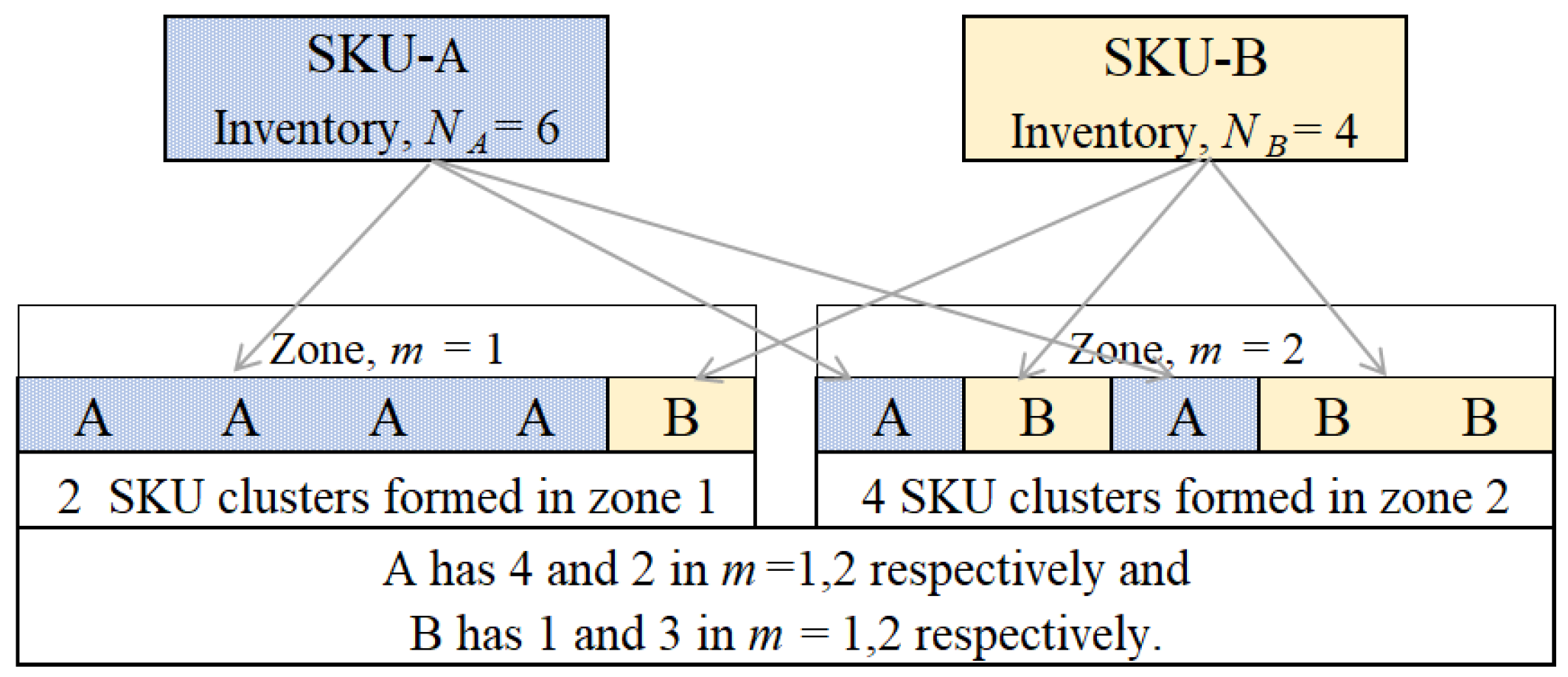
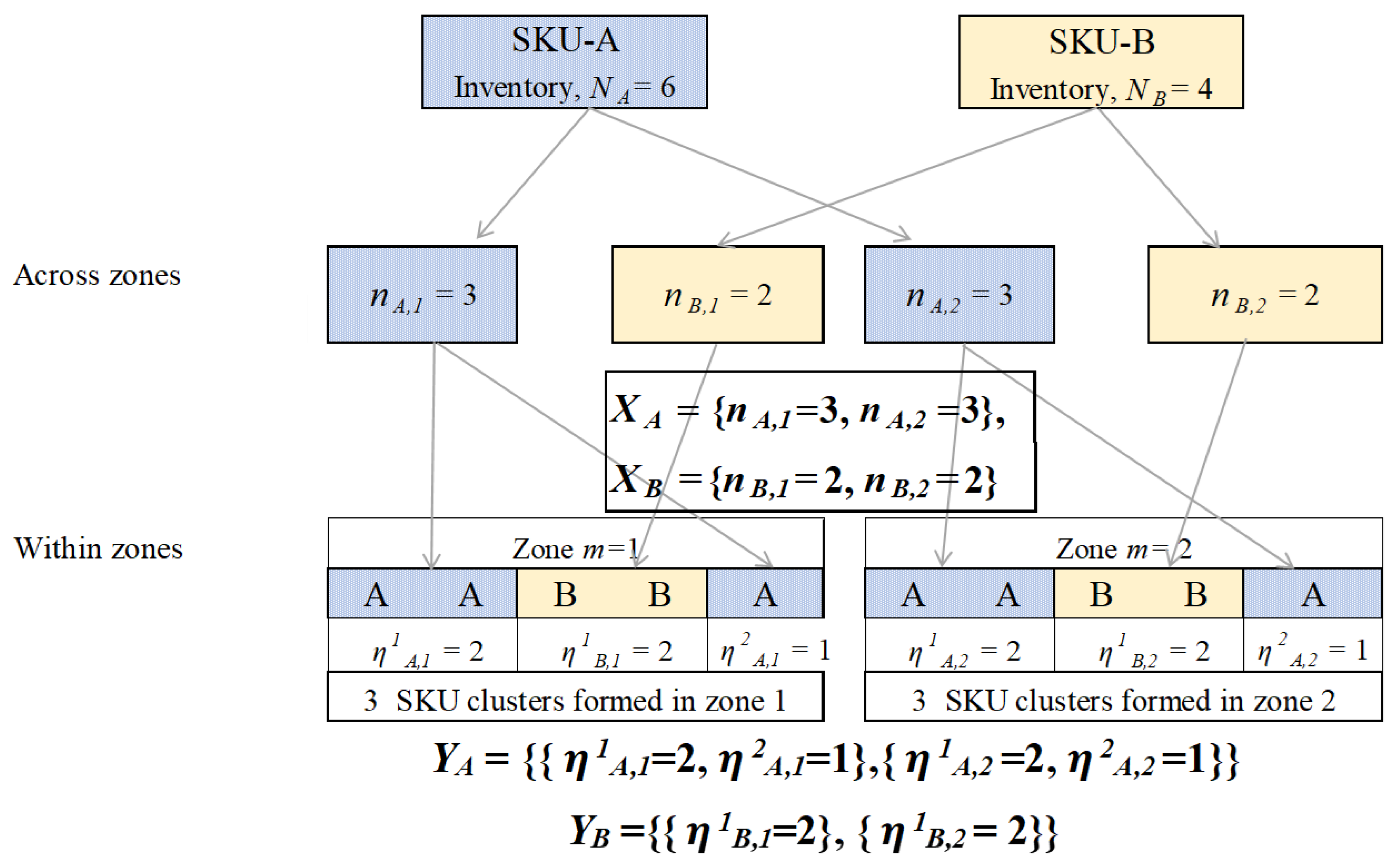
3.1.1. Across-Zone Scattering of Stock

This relates to the allocation of inventory of each SKU across various zones of the warehouse. The even scattering of SKU inventory across the geographical areas of a warehouse is essential for the widespread availability of products for order picking. Here, the specific decision involves the determination of inventory of each SKU i in each zone m, i.e., $n_{im}$, in a feasible manner. Let the set $X_i=\left\{n_{im},\forall m\right\}$ consist of values of $n_{im}$ arising from the split of inventory $N_i$ of SKU i into m zones, satisfying the location availability and the material balance constraint given by the equation below.

$$\sum _{m=1}^M{n}_{im}=N_i \forall i$$

(4)

3.1.2. Within-Zone Scattering of Stock

Scattered storage requires splitting the incoming inventory of each SKU into smaller put away lots. Each put away lot is assigned to a set of contiguous storage locations called a cluster (Section 2.1). The scattered storage assignment within zones requires splitting the inventory of SKU i in zone m, $n_{im}$, into multiple clusters of sizes ${\eta }_{im}^c$ for all c.

Let $Y_i=\left\{{{\rm Y}}_{im},\forall m\right\}, \mathrm{w}\mathrm{h}\mathrm{e}\mathrm{r}\mathrm{e} {{\rm Y}}_{im}=\left\{{\eta }_{im}^c,\forall c\right\}$ is a set of sets consisting of values of ${\eta }_{im}^c$ arising from splitting inventory N_i of SKU i into different clusters across the different zones. Entries of the set $Y_i$ follow the restrictions on the storage location availability, cluster definition, and material balance constraint given by the equation below:

$$\sum _{m=1}^M\sum _{c=1}^{\left|{{\rm Y}}_{im}\right|}{\eta }_{im}^c=N_i \forall i$$

(5)

where

$$\sum _{c=1}^{\left|{{\rm Y}}_{im}\right|}{\eta }_{im}^c=n_{im} \forall i,m$$

(6)

Section 3.2 presents an illustration of scattering with the help of the sets defined above.

3.2. An Illustration of Hierarchical Scattering

In our hierarchical scattering approach, first, the total stock $N_i$ of each SKU $i$ is partitioned into its feasible, across-zone quantities defined by set X_i. The elements of set X_i satisfy Equation (4). Each element $n_{im}$ of set X_i is then further partitioned into sets ${{\rm Y}}_{im}=\left\{{\eta }_{im}^c,\forall c\right\}$ for each m and the details of the partitioning are contained in set Y_i. The elements of the set Y_i satisfy Equations (5) and (6). For the example discussed in Section 2.1, Figure 3 shows an even split of the inventory of each SKU between the two zones, followed by a further split within each zone into clusters.

3.3. Limitations of Existing Measures in Capturing Both within- and across-Zone Scattering

Both ER and β depend on the total number of clusters across the entire warehouse; therefore, they can be maximised by splitting the inventory of each SKU into the maximum number of clusters [14,26]. Thus, to maximise the number of clusters, every item of the same SKU must be placed such that its neighbouring locations contain a different SKU. For maximising the Ey measure, the total stock of each SKU must be split evenly across all zones [22]. We now use the existing measures to compare the cluster formations in Figure 1 (Section 2.1) and Figure 3 (Section 3.2). In Figure 1, there are a total of C = 6 clusters, as illustrated in the calculations in Section 2.1. In Figure 3, there are 3 clusters in zone 1 and zone 2, giving a total of C = 6 clusters. Thus, using the set theoretic analogy from Section 2.1 and Section 3.1.2, we know that ER and $\beta$ depend on the total cardinality of all the elements within sets Y_A, Y_B, i.e., we have

$$\left|{{\rm Y}}_{A1}\right|+\left|{{\rm Y}}_{A2}\right|+\left|{{\rm Y}}_{B1}\right|+\left|{{\rm Y}}_{B2}\right|=2+2+1+1=6.$$

Hence, the arrangements in Figure 1 and Figure 3 give the same values for the two measures ER and $\beta$ as those in Section 2.1. Ey, as defined by Pawar et al. [22], has different values for SKU arrangements in Figure 1 and Figure 3, as Ey depends on the contents of sets X_A and X_B, which are different between the cases of SKU arrangements. In Figure 1, the sets are

X_A = {n_A,1 = 4, n_A,2 = 2}, X_B = {n_B,1 = 1, n_B,2 = 3},

(7)

and, in Figure 3, the sets are

X_A = {n_A,1 = 3, n_A,2 = 3}, X_B = {n_B,1 = 2, n_B,2 = 2}

(8)

It is clear that measures ER and $\beta$ depend on the total cardinality of the elements of sets $Y_i \forall i$, whereas Ey depends on the values of the elements of sets $X_i \forall i$. However, hierarchical scattering involves the elements of both types of sets $X_i,Y_i$; hence, its nuances cannot be entirely captured by the earlier measures. In Section 4, we propose a measure of scattering that considers the elements of both sets $X_i, Y_i$ rather than just using the elements of one set and the cardinality of the other set.

3.4. Benefits of Hierarchical Approach towards Scattering

A closer examination of the scattering generated by the non-hierarchical approach in Figure 1 and the hierarchical approach in Figure 3 reveals some key differences between the two approaches, as elaborated below.

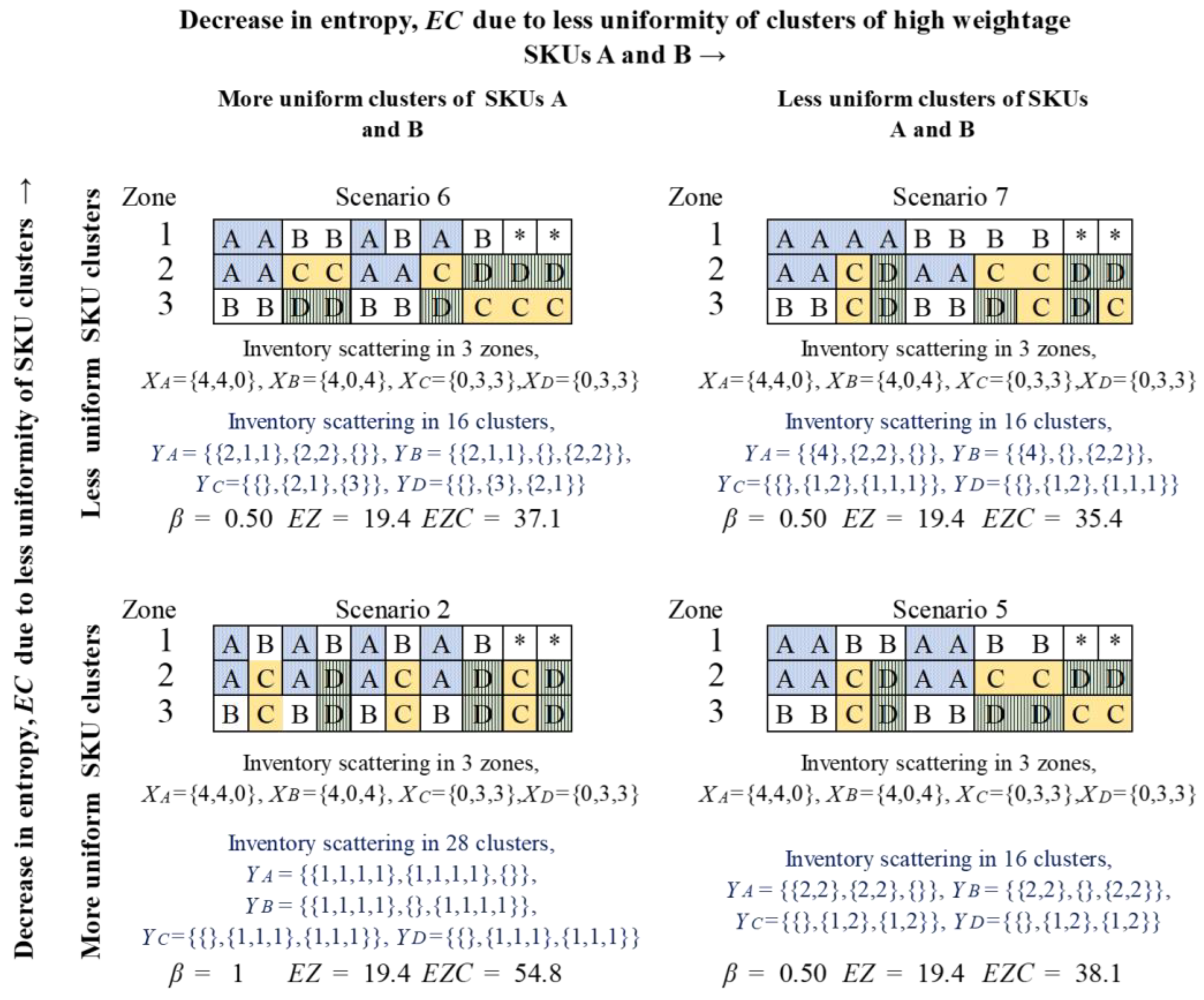
3.4.1. Uniformity of Scattering of SKU Inventory across Zones

For instance, the split of SKU inventory across the two zones, in Figure 1 and Figure 3, can be compared through sets X_A and X_B, as seen in Equations (7) and (8), respectively. Figure 1 represents uneven inventory scattering, Figure 3 represents even inventory scattering across the zones, and the latter is clearly more desirable. The first step in hierarchical scattering can control the evenness of across-zones scattering and, therefore, can be adapted for different situations, e.g., incorporating zone sizes in case the zones do not have an equal number of locations. The measures of ER and β do not capture the evenness of scatter across the zones. Ey does capture this effect, whereby a more even split of inventory across zones results in a higher value of Ey [22].

3.4.2. Uniformity in Size of Clusters for Each SKU within Zones

Once each SKU is split across the zones, the second step in the hierarchical scattering is to allot individual clusters of the SKU inventory to a zone. It is desirable that clusters for each SKU are uniform in size, which can be validated with the arrangements in Figure 1 and Figure 3. The cluster splits for SKUs A and B in Figure 1 are given by

$$Y_A={\{{\rm Y}}_{A1},{{\rm Y}}_{A2}\}= \left\{\right\{{{\eta }^1}_{A,1}=4\}, \{{{\eta }^1}_{A,2}=1, {{\eta }^2}_{A,2}=1\left\}\right\},$$

$$Y_B=\{{{\rm Y}}_{B1},{{\rm Y}}_{B2}\}=\left\{\right\{{{\eta }^1}_{B,1}=1\}, \{{{\eta }^1}_{B,2}=1, {{\eta }^2}_{B,2}=2\left\}\right\},$$

(9)

and the cluster splits for Figure 3 are given by

$$Y_A={\{{\rm Y}}_{A1},{{\rm Y}}_{A2}\}= \left\{\right\{{{\eta }^1}_{A,1}=2, {{\eta }^2}_{A,1}=1\}, \{{{\eta }^1}_{A,2}=2, {{\eta }^2}_{A,2}=1\left\}\right\},$$

$$Y_B=\{{{\rm Y}}_{B1},{{\rm Y}}_{B2}\}=\left\{\right\{{{\eta }^1}_{B,1}=2\}, \{{{\eta }^1}_{B,2}=2\}$$

(10)

ER and β consider only the number of clusters of inventory, i.e., the total cardinality of all the elements of sets Y_A and Y_B, which is the same in both Figure 1 and Figure 3. They do not consider the unevenness in their sizes, i.e., 3 clusters of SKU A of sizes (4, 1, 1) in Figure 1 as compared to 4 clusters of SKU A of sizes (2, 1, 2, 1) in Figure 3. Ey also does not capture the difference in cluster sizes within each zone.

Scattering with uniformity in cluster sizes is desirable for two reasons: First, during the order-picking process, the inventory in the clusters is depleted. Uniformity in cluster sizes helps with maintaining a high number of clusters and therefore a higher number of alternate picking locations, as the inventory is depleted. Second, uniformity in cluster sizes also helps with reducing picker travel. In Figure 3, for zone m = 1, a picker moving from left to right must cross 4 locations towards the right to reach SKU B, whereas for zone m = 1 in Figure 3, the picker can reach SKU B after crossing only 2 locations.

3.4.3. Total Number of Clusters for Each SKU

In order to achieve effective scattering, there should be an appropriate number of inventory clusters for each of the various SKUs stored in the warehouse. In practice, it may be desirable to have more clusters for SKUs with higher inventory to improve the order-picking performance. From this standpoint, the arrangement in Figure 3, given in Equation (10), which has four clusters of high-inventory SKU A, is preferable to the arrangement in Figure 1, given in Equation (9), which has only 3 clusters of SKU A.

Measures ER and β are based on the total number of clusters for all the SKUs together, irrespective of how many and which specific SKUs are contributing to the number of clusters. Ey, on the other hand, is insensitive to the number and size of the clusters. Hierarchical scattering provides control of the across-zone scattering and the within-zone creation of clusters at the SKU level and overcomes the limitations of the existing approaches.

Entropy is a commonly used measure for dispersion in many different fields of research, including logistics [27]. This motivated us to explore the application of entropy in the hierarchical scattering of stock to improve upon the above-mentioned limitations of the existing measures.

4. Developing an Entropy Measure for Hierarchical Scattering and Scattered Storage Policy

Shannon’s entropy has been widely used in diverse fields such as logistics [27], economics [28], medicine [29], and soil sciences [30]. It has origins in information theory, where it is used to measure the amount of information contained in a random variable [31], as shown in Equation (11),

$$E=-\sum _i{P}_i\mathrm{l}\mathrm{n}\left(P_i\right)$$

(11)

where P_i represents the probability associated with the ith value of the random variable, and ${\sum }_i{P}_i=1$.

Shannon’s entropy measures the evenness of the distribution of probabilities across various outcomes of an event. The maximum value of Shannon’s entropy is achieved if the probabilities are uniformly distributed across all possible values, representing the highest uncertainty in the value of the random variable [32]. In the next two sections, we conceptualise two entropy measures to quantify the two components of scattering discussed in Section 3. This is followed by the development of an expression for the total entropy of stock arrangement.

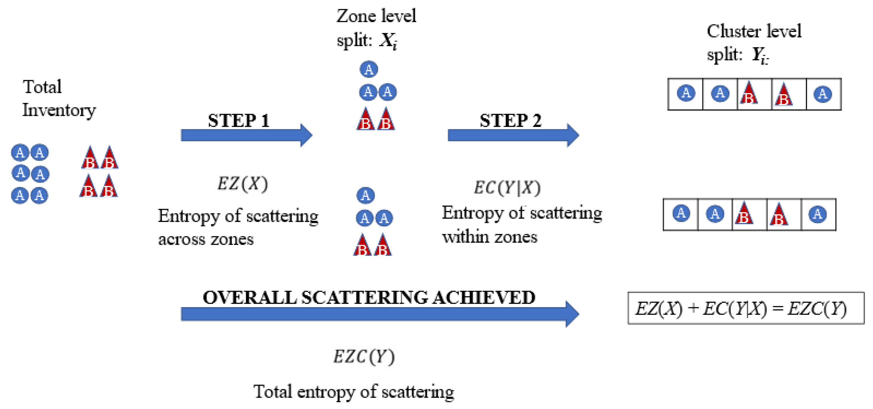
4.1. Entropy of Scattering across Zones: EZ

We use the entropy of scattering across zones, EZ, as a measure of the scattering of stock across different zones of the warehouse, which is the first step in the hierarchical scattering explained in Section 3. This measure, as defined by Pawar et al. [22], uses the elements of set $X_i \forall i$. They suitably modify Equation (11) to define the entropy of inventory arrangement across zones for SKU i, EZ($X_i$), as shown in Equation (12).

$$EZ\left(X_i\right)=-\sum _{m=1}^M\frac{n_{im}}{N_i}\mathrm{l}\mathrm{n}\left(\frac{n_{im}}{N_i}\right)\forall i$$

(12)

Accordingly, the EZ for the entire warehouse is obtained by taking a weighted sum of EZ($X_i$) across all SKUs, using the total inventory of each SKU, with N_i as its weight.

$$EZ\left(X\right)=\sum _{i=1}^I{N}_i\times EZ\left(X_i\right)=\sum _{i=1}^I{N}_i\left(-\sum _{m=1}^M\frac{n_{im}}{N_i}\mathrm{l}\mathrm{n}\left(\frac{n_{im}}{N_i}\right)\right)$$

(13)

Equation (13) can be further simplified to the following form:

$$EZ(X)=-\sum _{i=1}^I\sum _{m=1}^M{n}_{im}\mathrm{l}\mathrm{n}\left(n_{im}\right)+\sum _{i=1}^I{N}_i\mathrm{l}\mathrm{n}{(N}_i)$$

(14)

Notably, the second term in Equation (14) is a constant for a given SKU-level inventory of the warehouse and is not impacted by the inventory arrangement across zones. However, the first term in Equation (14) depends on the inventory distribution across zones. A higher entropy arrangement distributes the inventory more uniformly across zones, leading to more alternative locations for picking every SKU. Conversely, a higher entropy arrangement leads to a greater number of SKUs in each zone, which increases the possibility of completing a pick list within fewer zones. The maximum entropy of stock arrangement is achieved when the stock of each SKU is uniformly distributed across all zones, and this can be used to find the upper bound on the entropy (see properties below). Thus, the entropy EZ measures the evenness of allocation of incoming SKU stock across various zones.

4.2. Entropy of Scattering within Zones: EC

In this section, we present another entropy-based measure that quantifies the extent of scattering within zones that is achieved through the formation of SKU-level clusters. This measure considers the uniformity of the sizes of clusters and their distribution across various SKUs within a zone. As discussed in Section 3, the clusters are formed in the second step of hierarchical scattering. Here, the allocation of each SKU i in each zone m given by $n_{im}$ in set $X_i$ is further split into ${\eta }_{im}^c$ clusters, which are listed in set ${{\rm Y}}_{im}$ within set $Y_i$.

We define an entropy, EC, that captures the scattering of the second step in the hierarchical scattering for SKU i in zone m, given the allocations as per the first step, $X_i=\left\{n_{im},\forall m\right\}$

$$EC\left({{\rm Y}}_{im}|n_{im}\right)=-\sum _{c=1}^{\left|{{\rm Y}}_{im}\right|}\frac{{\eta }_{im}^c}{n_{im}}\mathrm{l}\mathrm{n}\left(\frac{{\eta }_{im}^c}{n_{im}}\right)$$

(15)

$EC\left({{\rm Y}}_{im}|n_{im}\right)$, as calculated above, is then weighted by each SKU’s inventory in zone m and summed over all SKUs i and zones m to give the total entropy of scattering within zones.

$$\begin{gathered} EC\left(Y_i|X\right)=\sum _{m=1}^M{n}_{im}\left(\sum _{c=1}^{\left|{{\rm Y}}_{im}\right|}\frac{{\eta }_{im}^c}{n_{im}}\mathrm{l}\mathrm{n}\left(\frac{{\eta }_{im}^c}{n_{im}}\right)\right) \\ EC\left(Y|X\right)=\sum _{i=1}^{I}EC\left(Y_i|X\right)=-\sum _{i=1}^I\sum _{m=1}^M{n}_{im}\left(\sum _{c=1}^{\left|{{\rm Y}}_{im}\right|}\frac{{\eta }_{im}^c}{n_{im}}\mathrm{l}\mathrm{n}\left(\frac{{\eta }_{im}^c}{n_{im}}\right)\right) \end{gathered}$$

(16)

Equation (16) simplifies to Equation (17) as

$$EC(Y|X)=-\sum _{i=1}^I\sum _{m=1}^M\sum _{c=1}^{\left|{{\rm Y}}_{im}\right|}{\eta }_{im}^c\mathrm{l}\mathrm{n}\left({\eta }_{im}^c\right)+\sum _{i=1}^I\sum _{m=1}^M{n}_{im}\mathrm{l}\mathrm{n}(n_{im})$$

(17)

Entropy EC in (17) captures the evenness in the clusters across the SKUs in each of the zones and is shown to have merit in Section 3. EC can be maximised by the creation of a large number of evenly sized clusters of each SKU within each zone. In the following two sections, we develop an expression for the total entropy of scattering and show how it relates to the two components of entropy discussed previously.

4.3. Total Entropy of Scattering across All Clusters in All Zones: EZC

The two components of scattering considered in Section 4.1 and Section 4.2 may be visualised as resulting from two sequential steps involved in splitting the SKU-level inventory of the warehouse, N_i, into clusters of size ${\eta }_{im}^c$ (Figure 4).

The total entropy of scattering across clusters for a particular SKU i, EZC($Y_i$), is accordingly defined in Equation (18) by using the elements of set $Y_i \forall i$.

$$EZC(Y_i)=-\sum _{m=1}^M\sum _{c=1}^{\left|{{\rm Y}}_{im}\right|}\frac{{\eta }_{im}^c}{N_i}\mathrm{l}\mathrm{n}\left(\frac{{\eta }_{im}^c}{N_i}\right) \forall i$$

(18)

Therefore, the total entropy of scattering across all clusters in the warehouse, EZC, is computed as the weighted sum of EZC($Y_i$) across all SKUs using the total inventory of each SKU, N_i, as the weight (19).

$$EZC\left(Y\right)=\sum _{i=1}^I{N}_i\times EZC\left(Y_i\right)=\sum _{i=1}^I{N}_i\left(-\sum _{m=1}^M\sum _{c=1}^{\left|{{\rm Y}}_{im}\right|}\frac{{\eta }_{im}^c}{N_i}\mathrm{l}\mathrm{n}\left(\frac{{\eta }_{im}^c}{N_i}\right)\right)$$

(19)

Equation (19) may be simplified to

$$EZC(Y)=-\sum _{i=1}^I\sum _{m=1}^M\sum _{c=1}^{\left|{{\rm Y}}_{im}\right|}{\eta }_{im}^c\mathrm{l}\mathrm{n}\left({\eta }_{im}^c\right)+\sum _{i=1}^I{N}_i\mathrm{l}\mathrm{n}{(N}_i)$$

(20)

The best possible cluster formation results in ${\eta }_{im}^c$ = 1 $\forall i$, m, c. Hence, EZC has an upper bound of ${\sum }_{i=1}^I{N}_i\mathrm{l}\mathrm{n}{(N}_i)$.

In the hierarchical scattering process, first, the inventory allocation across zones is performed for every SKU (sets $X_i \forall i$); it is then followed by within-zone cluster formation (sets $Y_i \forall i$). Thus, the scattering of inventory across and within zones through two hierarchical steps leads to the total entropy across clusters, EZC. EZ and EC, achieve two different kinds of scattering, which are complementary to each other and, therefore, are both desirable. From Equations (14), (17), and (20), one can see that the three entropies in the hierarchical scattering approach are related. This is shown in the properties of entropy as follows.

4.4. Some Properties for EZ, EC, and EZC

Property 1. 

$EZ \left(X\right)$ has an upper bound of N ln(M).

Proof of Property 1. 

In Equation (14), substitute $n_{im}=N_i/M$. This results in SKU i having the same stock across all m zones.

$$EZ(X)=-\sum _{i=1}^I\sum _{m=1}^M\frac{N_i}{M}\mathrm{l}\mathrm{n}\left(\frac{N_i}{M}\right)+\sum _{i=1}^I{N}_i\mathrm{l}\mathrm{n}\left(N_i\right)$$

$$EZ\left(X\right)=-\frac{1}{M}\left(\sum _{i=1}^I\sum _{m=1}^M{N}_i\ln N_i-\sum _{m=1}^M\left(\mathrm{l}\mathrm{n}\left(M\right)\sum _{i=1}^I{N}_i\right)\right)+\sum _{i=1}^I{N}_i\mathrm{l}\mathrm{n}\left(N_i\right)$$

$$EZ\left(X\right)=N\mathrm{l}\mathrm{n}\left(M\right)$$

□

Property 2. 

EC, EZ, and EZC are related.

Proof of Property 2. 

From Equations (14), (17), and (20), it can easily be shown that

$$EZ\left(X\right)+EC\left(Y\right|X)=EZC(Y)$$

(21)

□

Property 3. 

EZC is always greater than or equal to EZ.

Proof of Property 3. 

The value of EZC cannot be less than EZ in any stock arrangement. This can be proved using Equation (20). By definition, each entropy is non-negative, i.e., EZ, EC, EZ $\ge 0;EZC\ge EZ$. □

Property 4. 

EZC can be maximised sequentially.

Proof of Property 4. 

To achieve an even scattering of SKU inventory across the zones in a warehouse, we recommend a hierarchical method that first attempts to maximise EZ to obtain an optimal collection of sets X^*. Thereafter, EC is maximised to achieve scattering across a high number of evenly sized clusters within zones. These clusters are represented by the optimal collection of sets Y^* for the given optimal stock allocation to the zones X^*. Accordingly, using Equation (21), we compute the total entropy, EZC, in a hierarchical manner after setting the values of X to X^* and Y to Y^*,

$$EZC\left(Y^{\mathrm{*}}\right)=EZ\left(X^{\mathrm{*}}\right)+EC\left(Y^{\mathrm{*}}\right|X^{\mathrm{*}})$$

(22)

□

We suggest a heuristic method in Section 5 to accomplish these two steps to obtain a good value of EZC according to Equation (22).

4.5. Features of the Proposed Entropy Measures in Relation to the Existing Measures

In this section, we illustrate how the two proposed entropy measures, taken together, overcome the limitations of ER and β stated in Section 3.3. First, we show that the EZ for each SKU is not dependent merely on the presence of the SKU in a zone but also considers the uniformity of distribution of the SKU’s inventory across various zones.

Consider four SKUs, A, B, C, and D, with inventory of 8, 8, 6, and 6 units, respectively. A total of 28 units of inventory of these SKUs needs to be arranged in a warehouse. The warehouse is divided into 3 zones with 10 storage locations each, such that each zone is a group of contiguous locations. We considered the stock arrangements with progressively higher levels of scattering. This was achieved in two ways, as shown in Figure 5. First, we increased the scattering for each SKU from being spread across 2 aisles in scenarios 1 and 2 (depicted in the left column), to being spread across 3 aisles in scenarios 3 and 4 (shown in the right column). Empty locations are indicated with an asterisk (*). Next, we increased the evenness of the distribution of the stock across aisles in the scenarios in the bottom row (scenarios 2 and 4), and compared it to the corresponding scenarios in the top row (scenarios 1 and 3). We calculated ER, β, entropies (EZ), and (EZC) for each of the arrangements using Equations (1), (2), (14), and (20), respectively.

Notably, across all four scenarios, the values of both ER and β are 1, while EZC is 54.8, thereby reflecting the maximum possible scattering of stock. Thus, ER and β are not able to detect the differences in scattering among the four scenarios. However, the value of EZ does show sensitivity among the different scenarios in a consistent manner, i.e., EZ increases from top to bottom and from left to right across the different scenarios in Figure 5.

Similarly, Figure 6 captures the effect of cluster size and its distribution across SKUs on β, EZC, and EZ. ER was not computed as it followed a trend similar to β. We chose scenario 2 (discussed earlier in Figure 5) as our base scenario, having a total of 28 clusters of different SKUs, each comprising a single unit. From this scenario, we created three other scenarios, 5, 6, and 7, by consolidating the clusters in a controlled manner so that the total number of clusters reduced from 28 to 16 while maintaining the same inventory distribution of SKUs across different zones (Figure 6).

Since product allocation across zones did not change, EZ remained the same at 19.4 across all four scenarios. The values of β also remained the same at 0.50 in the three newly created scenarios (5, 6, and 7) because β depends only upon the number of clusters (which was 16 each for scenarios 5, 6, and 7) and not their distribution over the SKUs and sizes.

However, scenarios 5, 6, and 7 have different levels of scattering that are captured by EZC as follows. Scenario 5 has more evenly sized clusters than scenario 7; therefore, the EZC value for scenario 5 is higher than that for scenario 7. For the SKUs with higher inventory, i.e., SKUs A and B, scenario 7 has fewer and less evenly distributed clusters than scenario 6. For SKUs with a lower inventory, i.e., SKUs C and D, the situation is exactly the opposite. This is captured by a lower value of EZC for scenario 7 than in scenario 6. Thus, EZC is sensitive to the number and evenness of clusters at an overall level, as well as across different SKUs.

5. Entropy-Based Storage Location Assignment (ESLAP)

We modelled the hierarchical storage assignment problem as an entropy, EZC, maximisation problem. The notations used are mentioned in Section 3.1. The SKU inventory present in the warehouse before replenishment is reflected in the model by setting $Z_{ims }=1$, if SKU i is present in aisle m and location s. Let the following set define the initial SKU assignment of the warehouse before replenishment:

$${\mathcal{L}}_0=\left\{\left(i,m,s\right):Z_{ims}=1 \forall (i,m,s)\in \mathcal{H}\right\}.$$

where the details of the storage locations that are initially occupied are given in set

$$L_0=\left\{\left(m,s\right):\forall (i,m,s)\in {\mathcal{L}}_0\right\}$$

Note that some locations may be empty at this point of time, which is given by the set $L_E=L_A-L_0$. We initialise $Z_{ims }=0$ for all empty locations $(m,s)$ $\in L_E$ for all SKUs i $\in$ I_A. At the beginning of each day, if the stock of any SKU i is less than its stock norm N_i, then R_i units of SKU i are replenished, as shown below. Thus, the SKUs to be replenished are given by

$$I_R=\left\{i:\sum _{(m,s)\in L_0}{Z}_{ims}<N_i \forall i\in I_A\right\}$$

and

$$R_i=N_i-\sum _{\left(m,s\right)\in L_0}{Z}_{ims}, \forall i\in I_R.$$

Also, ${\sum }_{i\in I_R}{R}_i$ = R.

Using the above initialisations, we can now represent the nonlinear model for entropy maximisation given by the ESLAP.

ESLAP:

$$\mathrm{M}\mathrm{a}\mathrm{x}\mathrm{i}\mathrm{m}\mathrm{i}\mathrm{s}\mathrm{e} EZC\left(Y\right)=\sum _{i=1}^I{N}_i\left(-\sum _{m=1}^M\sum _{c=1}^{\left|{{\rm Y}}_{im}\right|}\frac{{\eta }_{im}^c}{N_i}\mathrm{l}\mathrm{n}\left(\frac{{\eta }_{im}^c}{N_i}\right)\right)$$

(23)

subject to the following constraints:

$$\sum _{\forall {s∊L}_{imc}}{Z}_{ims}={\eta }_{im}^c \forall i\in I_A \& m\in M_A \& c\in (1..\left|{{\rm Y}}_{im}\right|)$$

(24)

$$\sum _{\forall i\in I_R}{Z}_{ims}\le 1 \forall \left(m,s\right)\in L_E$$

(25)

$$\sum _{\forall \left(m,s\right)\in L_E}{Z}_{ims}=R_i \forall i\in I_R$$

(26)

$$\sum _{m=1}^M\sum _{c=1}^{\left|{{\rm Y}}_{im}\right|}{\eta }_{im}^c=N_i \forall i\in I_A$$

(27)

$$Z_{ims}\in \left\{0,1\right\} \forall i\in I_R\&(m,s)\in L_E$$

(28)

The objective function (23) seeks to maximise the EZC. Constraint (24) counts the number of SKU i in a particular cluster c in zone m. Constraint (25) ensures that only one SKU is assigned to a particular location. Constraint (26) ensures that the total inventory of SKU i assigned to empty locations is equal to the replenishment inventory of SKU i. Constraint (27) ensures that the total stock of each SKU in all clusters across all zones is equal to its stock norm. Constraint (28) represents the binary decision variable.

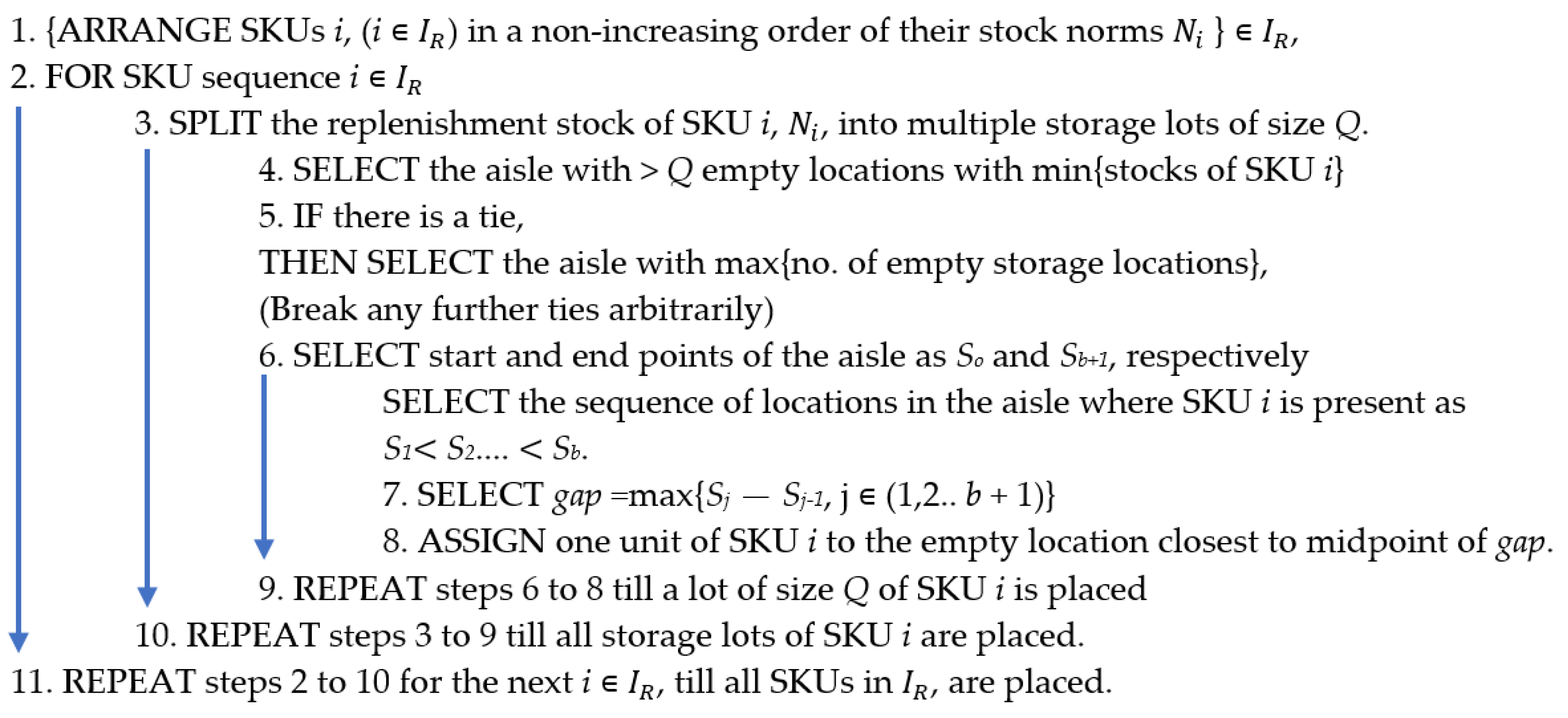
5.1. Proposed Heuristic for Scattered Storage Assignment Policy (SSP)

We propose a storage assignment heuristic (SSP) that scatters the inventory of each SKU with an aim of maximising entropy EZC as per Equation (21). SSP uses a lot size parameter, Q, to control the degree of scattering across zones, and, accordingly, we refer to the storage assignment heuristic as SSP(Q). The procedure begins with splitting the incoming stock of every SKU into storage lots of size Q.

For each SKU, SSP(Q) allocates the storage lots to various aisles to maximise the uniformity of the distribution of the inventory of the SKU across aisles, thereby maximising EZ. Next, the SKU assigned to the aisle is placed in empty storage locations to create the maximum number of SKU clusters, thereby maximising EC. The heuristic assigns each unit of the SKU to an empty storge location that is most distant from any other position occupied by the same SKU in that aisle. These two hierarchical steps of the heuristics are executed using the algorithm in Figure 7.

5.2. Comparison of the Heuristic with Genetic Algorithm Meta Heuristic

The formulation of the ESLAP as a nonlinear integer programming (NLIP) problem is acknowledged to be NP-hard [33,34], presenting significant challenges for conventional solvers. The commonly used solvers do not accept the objective function in logarithmic form and require workarounds like piecewise linear or quadratic approximation by introducing auxiliary variables. Therefore, we explored a metaheuristic approach using a genetic algorithm (GA) to solve the ESLAP.

We considered three different warehouse sizes—comprising 50, 300, and 900 locations, each examined under four distinct levels of inventory depletion prior to replenishment ranging from 25% to 100% empty. For every scenario, we conducted five trials. The computation time for each GA trial was capped at an upper limit of 1800 s.

The results, averaged across the five trials, show the relative performance of the SSP(Q = 1) algorithms in terms of entropy achieved and computational efficiency, as summarized in

Table 3. Comparison of solution quality and performance between SSP(Q = 1) and genetic algorithm.

		SSP(Q = 1)	Genetic Algorithm
Warehouse Size (# of Storage Locations)	Initial Warehouse Occupancy	Entropy *	Entropy (% Improvement (+ve) over SSP(Q = 1))	(Computational Time in Seconds, # of Generations)
Size 1 (50)	25%	83.3	85.0, (+2.0%) **	(49, 51)
	50%	85.0	85.2, (+0.3%)	(56, 51)
	75%	87.5	87.5, (+0.0%)	(67, 52)
	100%	87.8	87.8, (+0.0%)	(82, 53)
Size 2 (300)	25%	1025.9	1029.9, (+0.4%)	(252, 81)
	50%	1044.3	1044.8, (+0.1%)	(590, 122)
	75%	1055.5	1057.5, (+0.2%)	(1216, 153)
	100%	1051.1	1058.0, (+0.7%)	(1500, 127)
Size 3 (900)	25%	4052.4	4055.5, (+0.1%)	(1714, 144)
	50%	4116.7	4086.2, (−0.7%)	(1800, 52)
	75%	4141.0	4072.9, (−1.6%)	(1800, 19)
	100%	4136.1	4049.5, (−2.1%)	(1800, 10)

* Computation time is a fraction of a second. ** Entropy in bold indicates best performance for a configuration.

. For the two smaller configurations, size 1 and size 2, the performance of the genetic algorithm is superior or the same as that of the SSP(Q = 1) heuristic. However, the difference between the two is only 0.5%. In these smaller problems, the stopping criterion for genetic algorithm was a lack of improvement in objective function. In contrast, for the size 3 warehouse, for an emptiness of 50% and above, the performance of genetic algorithm was worse by 1.5% compared to the heuristic. In these cases, the stopping criterion for genetic algorithm was exceeding the solve times.

It is evident that as the problem size increased due to a larger warehouse or more empty locations, the performance of the genetic algorithm within the specified time limit deteriorated. For the warehouse sizes considered here, the heuristic gave very good solutions within a fraction of a second. Given the scale of real-world applications, which are likely to far exceed the sizes of the instances examined in this study, the SSP(Q = 1) heuristic emerges as a viable and effective solution strategy for solving the ESLAP.

The computations were conducted in MATLAB R2023a.

6. Simulation Study

In this study, we designed a simulation to assess the performance of the proposed entropy-based hierarchical scattered storage assignment.

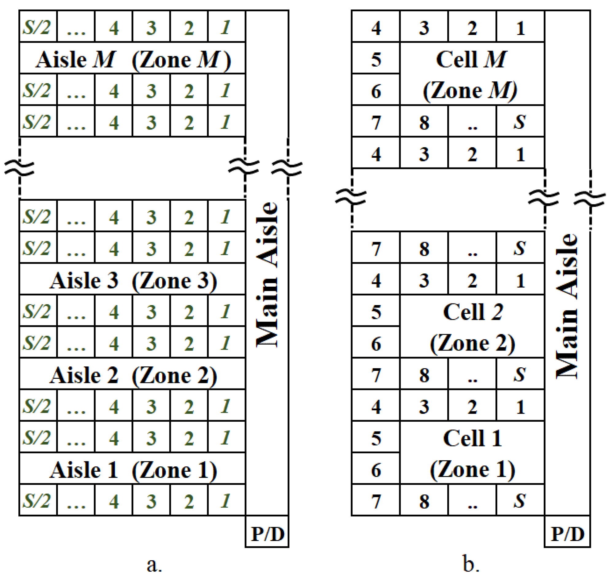
6.1. Warehouse Setup

We considered a rectangular picker in a parts warehouse comprising M zones, with each zone having S storage locations (Figure 2a). Each storage location could, at the most, store one unit of any SKU from I different SKUs. Each SKU’s inventory norm (planned inventory level in the warehouse) was proportional to the level of its demand, and the inventory norms across all SKUs added up to the total warehouse capacity (M × S). Order pickers started from the pickup/drop location, visited the pick locations as per the assigned pick list, and brought the picked stock back to the pickup/drop location following a return routing policy [35].

At the beginning of each day, the stock of each SKU was replenished to its stock norm from a central reserve area. The incoming stock were assigned to storage locations based on a specified storage assignment policy, which could either be the SSP(Q) (Section 5.1) or the benchmark COL (closest open location) policy (Section 6.2.1). The replenishment of the warehouse was followed by the order-picking operation. The demand orders on the warehouse were simulated from a 50:30 Pareto distribution. The daily pick load of the warehouse comprised W single-item orders. The warehouse followed a waveless picking strategy, i.e., the orders were considered for picking in the sequence of their arrival. All picker carts had the same size and could hold K items at a time. The incoming orders, in the sequence of arrival, were assigned to pickers in lots of K items each. The selection of pick locations and routing of pickers was conducted through the heuristic discussed in Section 6.2.2.

6.2. Benchmark Storage Assignment Policy and Order-Picking Heuristic

6.2.1. Closest Open Location Assignment (COL) Policy

A commonly used method for storage assignment of the incoming SKUs is the COL policy [4,18]. We have also witnessed the use of the COL policy in our visit to a large e-commerce warehouse. Under this policy, the worker assigns incoming inventory to the empty storage locations nearest to the pickup/drop location. This approach has an intuitive appeal for workers as it minimises their effort in replenishing stock. The COL policy, without deliberate lot splitting, was used as a benchmark for comparing the performance of the proposed scattered storage assignment policy, which aims to scatter the stock by maximising both EZ and EC. By coincidence, the COL approach may allow some stock scattering due to location availability constraints.

The algorithm used to simulate the COL policy was as follows:

• Step 1: List the SKUs present in the incoming stock in the nonincreasing order of the SKU-level stock norms. Consider the first SKU for storage assignment.
• Step 2: Select the aisle that is closest to the pickup/drop location and has one or more empty locations.
• Step 3: In the selected aisle, assign the stock of the SKU under consideration to the empty locations in ascending order of their distance from the main aisle. If the selected aisle becomes filled, select the next closest aisle to the pickup/drop location with one or more empty locations.
• Step 4: If all stock of the SKU under consideration is assigned to storage locations, move to the next SKU in the list until all the incoming stock is assigned.

6.2.2. Order-Picking Heuristic

The order-picking operation requires the selection of pick locations from the multiple choices available for each item in the pick list. It is desirable to complete the picklist within a short picking distance. Accordingly, we use a picking heuristic that attempts to minimise the number of aisles (zones) from which the items in a cart are picked. The picking heuristic is similar to the aisle-by-aisle heuristic for multi-item picking, where dynamic programming is used to select the sequence of aisles to be visited [36]. In our case, we select the aisles using a greedy procedure as described below. For every cart release, the following steps are followed for selecting the pick locations:

• Step 1: For each aisle, calculate the number of items from the cart that are available in the aisle for picking. Select the aisle with the availability of the maximum number of available items. In case of a tie, select the aisle closest to the pickup/drop location.
• Step 2: For each item available in the selected aisle, select the pick location containing the item closest to the main aisle.
• Step 3: Remove the items found in the aisle selected in Step 2 from the pending items of the cart. If the cart has any items where the pick location has not been identified, proceed to Step 1.
• Step 4: Create the picking route for the worker, starting and ending at the pickup/drop location and visiting each aisle with pick locations only once.

6.3. Different Simulated Warehouse Operating Conditions

We considered a warehouse with a fixed storage capacity of 900 storage locations (M), sufficient to hold the stock of all I SKUs as per their inventory norms. The warehouse considered here was small enough for a single picker to traverse. Other warehouse operating parameters were varied, as summarised in

Table 4. Different warehouse operating conditions simulated.

Warehouse Parameter	Values/Settings
SKU density (Hs %)	5.56, 11.11, 22.22, 33.33
Number of locations per aisle (S)	10, 25, 50, 75, 100
Workload (number of daily orders) (W)	300, 500
Picker cart size (K)	5, 10, 15, 20, 25

and explained next.

We defined the SKU density H_s = I/(M × S) × 100, which is the average number of different SKUs per 100 storage locations. An H_s of 5.56% implies that a range of 50 SKUs (I) is stored in the warehouse with 900 locations. In the simulation, we varied H_s from 5.55% to 33.33%, which covered an adequate range of the number of SKUs stored in the simulated warehouse. The number of locations in an aisle of the warehouse may also influence the effectiveness of scattering. Accordingly, five settings of the number of locations per aisle (S) were considered—10, 25, 50, 75, and 100. Researchers [35,37] have demonstrated that cart size influences the order-picking performance of a warehouse. Hence, our study considered five different cart sizes (K): 5, 10, 15, 20, and 25.

We surmised that lower values of storage lot size Q would result in more clusters for each SKU and, therefore, the higher scattering of stock. Different values of the storage lot size Q can be used to achieve stock arrangements with different levels of scattering. Through experimentation, we found that the simulation results did not vary appreciably for a value of Q greater than 20 but were sensitive at low values of Q. Accordingly, a total of 13 SSP(Q) for Q values equal to 1, 2, 3, 4, 5, 7, 9, 11, 13, 15, 20, 25, and 30 were considered in the simulation. The 240 different combinations of Hs, S, W, and K (Table 4) were simulated for the 13 SSPs and the COL policy, resulting in a total of 3360 (240 × 14) simulation runs.

6.4. Simulation Steps

The warehouse operations were simulated for 150 days for each of the 3360 configurations on MATLAB version R2021b. The steps followed for each simulation run were as follows:

• Start with a filled warehouse with all 900 locations occupied with an inventory of I SKUs as per their inventory norms. Obtain the initial stock arrangement by using SSP(Q = 1) on an empty warehouse. Use the same initial stock arrangement for all simulation runs.
• Measure the entropy of the stock arrangement. Complete the order picking for the day’s picking workload (W). Measure the order-picking travel distance.
• On the next day, replenish the warehouse to the stock norms using the specified storage assignment policy, measure the entropy of stock arrangement, and proceed with order picking. Measure the order-picking travel distance.
• Repeat step 3 for 150 days. Report the data of the last 100 days of simulation to remove the effect of the initial transient phase.

6.5. Performance Measures and Parameters

We measured the extent of the scattering of the stock arrangement by calculating entropies, i.e., EZ and EZC, per Equations (14) and (20), after the daily stock replenishment cycle during the period of simulation. We also tracked the following:

Picker travel distance: Picking travel distance has a direct impact on order-picking cost and time. We report the average pick distance per item picked in the warehouse as DP. One unit of DP is equal to the width of a storage location. Based on previous research [15], a high level of scattering is expected to reduce DP.

Parameters: Warehouse parameters such as cart size K, SKU density H_s, and the daily workload W have a bearing on DP. An increase in the cart size, K, is expected to reduce the DP as more items are picked in every picker trip. However, a larger cart size results in higher wait times as the picked items wait for the cart to be completely picked before commencement of order consolidation and shipping activities [14]. From our experience with e-commerce retailers, we believe that the SKU density in a picking area would affect the DP, so we studied the same. Moreover, the daily workload W determines the level of emptiness of the warehouse before replenishment begins [15]. We studied this effect in our simulations because DP is expected to increase progressively as the warehouse empties. At the same time, an emptier warehouse offers more opportunity to scatter the inventory effectively.

We present the simulation results in the next section.

7. Results

The results of this study are presented in three parts. Section 7.1 and Section 7.2 present the total entropy of stock arrangement and order-picking effort, respectively, for different levels of scattering obtained by SSP by controlling Q. Section 7.3 covers the impact of various warehouse parameters on the order-picking performance with the scattered storage assignment policy.

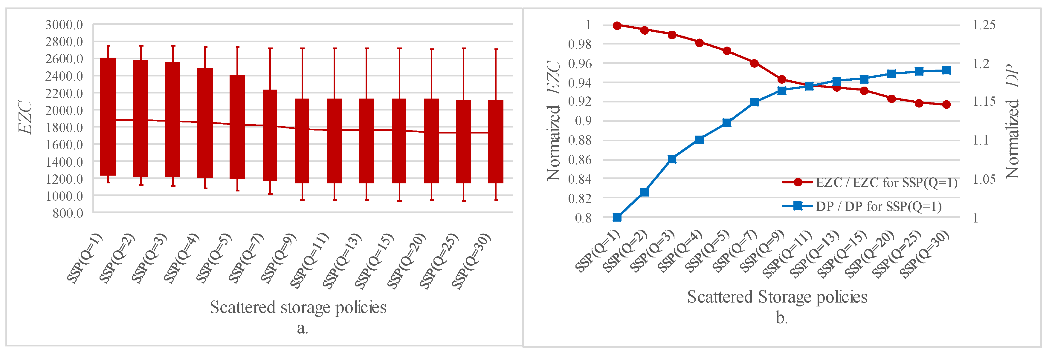
7.1. Variation in the Total Entropy (EZC) with Different Levels of Scattering

In our study, we varied the lot size Q to control the level of scattering in SSP(Q). For each SSP(Q), the EZC obtained using various combinations of simulation settings (Table 4) is plotted as a box and whisker plot in Figure 8a. The chart shows the variation in EZC across 13 SSP(Q) combinations considered in the simulation. We can observe that increasing the value of Q from 1 to 30 in SSPs results in progressively lower values of EZC.

Next, the average value of EZC for each SSP(Q) was calculated across all combinations of warehouse parameters. Figure 8b presents the average EZC for every SSP(Q), as a percentage of the average EZC for SSP(Q = 1). This normalised average EZC degrades by about 8% for the worst scattering scenario (Q = 30) compared to the highest scattering scenario (Q = 1).

7.2. Variation in Picking Performance with Different Levels of Scattering

Here, we present the order-picking performance, measured through distance per pick DP, for various SSP(Q) policies. First, we plot the normalised DP for various SSPs by dividing DP for each SSP by DP for SSP(Q = 1) in Figure 8b. The normalised DP is inversely correlated to the normalised EZC, with the correlation being −0.95. Next, we consider DP for the closest open location policy, DP(COL), as a benchmark to evaluate the order-picking performance of SSPs. Accordingly, in Figure 9, we report the average DP for each SSP as a fraction of DP(COL). The average DP for each SSP(Q) was calculated over all 240 combinations of warehouse parameters simulated in this study. Values less than one signify an improvement in performance over DP(COL) policy. It can be observed that the performance of entropy-based SSPs is superior to that of DP(COL) across the entire range of Q’s considered in the simulation. Moreover, the order-picking performance of SSPs deteriorates with an increase in Q. For the highest entropy SSP(Q = 1), the DP improves around 38% over DP(COL), with the improvement reducing to 26% for SSP(Q = 30).

7.3. Sensitivity of Pick Distance to the Warehouse Operating Parameters

In the previous section, we noted that SSP(Q = 1) performed the best on scattering and order-picking performance amongst all SSPs. Therefore, in this section, we consider the simulation results only for SSP(Q = 1) to study the impact of various operating parameters on the order-picking performance.

The picking demand on the warehouse is characterised by the daily picking workload (W) and SKU range, measured through SKU density (H_s). In

Table 5. Variation in DP with K and Hs for two different W values.

Cart Size	Workload	SKU Density
		Reference Case, Hs = 5.56%	Hs = 11.11%	Hs = 22.22%	Hs = 33.33%
		DP (Hs = 5.56%)	% Increase in DP over DP (Hs = 5.56%)
K = 5	W = 300	38.2	20%	48%	64%
	W = 500	41.9	19%	42%	55%
K = 10	W = 300	24.7	26%	59%	80%
	W = 500	27.3	23%	52%	69%
K = 15	W = 300	19.1	28%	65%	90%
	W = 500	21.5	25%	56%	76%
K = 25	W = 300	16.0	30%	69%	95%
	W = 500	17.8	27%	61%	81%
K = 25	W = 300	14.0	30%	71%	98%
	W = 500	15.5	28%	63%	85%

, we illustrate the sensitivity of the average pick travel distance per item, DP, to changes in H_s and W, for different values of cart size K. The first column in Table 5 represents DP for H_s = 5.56%, and the subsequent columns represent the percentage deterioration in DP with the corresponding increase in H_s. The DP reported below is an average of all combinations of S used in this study.

The first increase in H_s by 5.56% increases DP by 19–38% for various combinations of K and W. Furthermore, every 10% increase in H_s in the next two columns results in a corresponding increase in DP by approximately 42–71%, and 55–98%, respectively. This shows a significant increase in picking travel with an increase in the number of SKUs stored in the warehouse. Overall, increasing the SKU density by roughly 28% from its base value at 5.55% almost doubles DP.

An increase in workload from W = 300 to W = 500 increases the average pick distance per item by two to three units. A higher daily workload results in more emptying of the warehouse before replenishment, i.e., from 33.33% empty at W = 300 to 55.55% empty at W = 500, thus requiring pickers to travel longer distances. Also, increasing the cart size K reduces the average pick distance per item. An increase in the cart size K from 10 to 15 reduces the DP by four to five units. A similar increase in K from 15 to 20 results in diminishing benefits in DP of about two units or less.

8. Discussion and Managerial Implications

Amongst the various SSPs, we expected the SSP with Q = 1 to offer the highest level of scattering amongst all SSPs, as placing inventory in storage clusters of a single unit can offer the highest level of scattering. Higher Q values result in inventory being stored in larger storage clusters, resulting in lower scattering. This variation in the extent of scattering is captured well by the EZC in Figure 8a,b.

Also, as seen in Figure 8b, the normalised EZC values tend to drop with an increase in Q for lower values of Q. However, they tend to flatten out for Q > 20. This is because SSPs with lower values of Q (say, from Q = 1 to Q = 11) lead to different levels of scattering due to different sizes of storage clusters (Q). However, the higher Q values are higher than the stock norm for many SKUs. Hence, the entire stock of those SKUs is stored as a single lot for all SSPs with higher values of (Q). This leads to relatively less change in the level of scattering with values of Q higher than 20.

The range of SSPs between Q = 1 and Q = 11 represents the practical range of SSP that is likely to be used in a real-life application of scattered storage. In this range, we observe a strong correlation between the normalised values of EZC and Q, with the correlation coefficient being −0.93. Therefore, we can conclude that EZC adequately captures the varying extents of scattering obtained with different storage lot sizes. The highest level of scattering is obtained with Q = 1, with a progressive reduction in scattering with an increase in Q. Warehouse managers need to choose Q such that the need to increase scattering is balanced with the feasibility of performing put away for the selected Q.

We also observed an increase in DP with an increase in Q (Figure 9). However, even for high Q values, SSP is better in terms of picking travel than the closest open location policy. This shows that a deliberate attempt at scattering, even with a high put away lot, improves order-picking performance. The significant negative correlation (−0.95) between DP and EZC values suggests that targeting maximisation of EZC can result in a reduction in DP. Similar to EZC, the DP tends to flatten out for Q > 20 for the same reasons as discussed for EZC. We can conclude that the EZC of a stock arrangement can be used as an indicator to estimate the order-picking effort.

Warehouse managers need to carefully assess the SKU density, H_s, in the picking area, as an increase in H_s results in a significant increase in DP (Table 5). The SKU density can be reduced by moving a part of the SKU range to an alternate picking area, provided the lower number of SKUs justifies the workload of the pickers assigned to each area. We see a reduction in DP with an increase in K. For a higher K, the component of DP that is fixed for the trip, i.e., travel from and to the pickup/drop location, is allocated over a higher number of items in the cart. The contribution of this fixed component to DP reduces progressively with an increase in cart size, thus resulting in diminishing benefits from the increase in cart size.

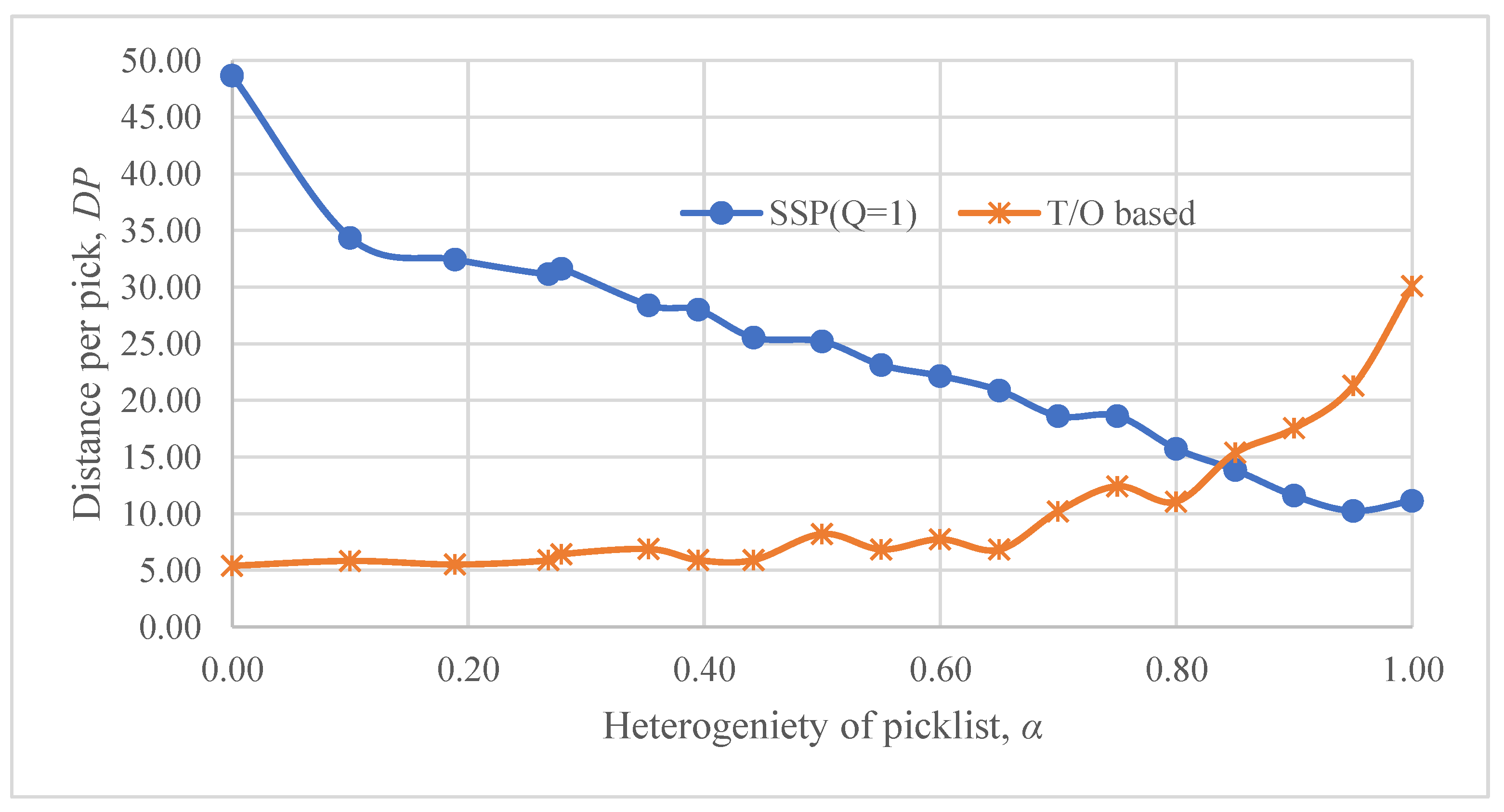
Impact of Picklist Diversity on the Performance of Various SSPs

The adoption of scattered storage hinges on the assumption that the picklists are highly diverse. Picklist diversity provides an advantage for scattered storage over traditional single-lot storage policies, as scattering makes a variety of SKUs accessible within a short picking distance. However, a less-diverse picklist may require the picker to travel to distant storage locations to pick the same SKU, hence increasing the picking travel. Therefore, managers must consider the diversity of picklist before making a decision on the adoption of scattered storage.

Weidinger (2018) defines heterogeneity of picklist, α, as

$$\alpha =1-\sum _{i∊I_K}\frac{Q_i\ast \left(Q_i-1\right)}{K\ast \left(K-1\right)}$$

where K is the size of picklist (maximum cart size in our simulation), Q_i is the number of units of SKU i in the picklist, and $I_K$ is the set of all SKUs present in the picklist. Here, α measures the probability that two randomly chosen items from the picklist are not of the same SKU. A high value of α implies highly diverse picklists and vice versa.

In our earlier simulation, the average α for the picklists was 0.96, and 99% of the picklists had an α value of higher than 0.9. This represents a high level of diversity commonly seen in the fulfilment warehouses of fashion industry and horizontal platforms like Amazon. These warehouses receive a high number of mostly a single unit per SKU order across tens of thousands of SKUs in the same picking area. However, this degree of picklist diversity may not be prevalent in warehouses serving other industries, which can be due to the lower number of SKUs or high demand skew across SKUs or customer ordering patterns.

To understand the impact of picklist diversity on the performance of a scattered storage policy, we conducted picking trials with picklists with different levels of α. For each picklist, we used an initially empty warehouse filled using (a) SSP(Q = 1) and (b) the COL policy with SKUs being considered for storage assignment in nonincreasing order of their turnover (T/O). The latter replicates the storage assignment achieved through a T/O-based policy, as the highest-turnover SKUs are placed in the closest available locations. We considered 10 picklists of 20 items each, for each level of α ranging from 0 (no heterogeneity) to 1 (highest heterogeneity). Figure 10 shows the DP obtained for both policies for picklists with different α values.

For picklists with an α of less than 0.85, the traditional T/O-based storage assignment gives superior results than the scattered storage policy; however, for picklists with an α greater than 0.85, the scattered storage policy performs better (Figure 10). The difference between the T/O-based storage policy and the scattered storage policy is quite stark for different values of α. Hence, warehouse managers need to carefully assess the heterogeneity of picklists before selecting the storage assignment policy for the warehouse. The results also highlight the picking inefficiency that may arise if a warehouse configured for servicing e-commerce orders with high heterogeneity is utilised to serve bulk orders with less SKU diversity, and vice versa.

9. Conclusions

The rapid expansion in e-commerce and the increasing prevalence of e-commerce warehouses underscore the need for making e-commerce warehouse operations sustainable from employee health and safety perspectives. This study proposed a novel approach for scattered storage and demonstrated that it can greatly reduce picking travel for e-commerce warehouse workers. It proposed a new entropy-based measure of scattering that addresses the shortcomings of the existing measures. A two-step hierarchical scattering approach was developed, where SKU inventory is first spread across the warehouse, followed by the formation of SKU storage clusters in each part of the warehouse. It was shown that the overall entropy-based measure of scattering is the sum of two measures that capture the effectiveness of each step. Managers can use these measurements to identify which aspect of scattering needs improvement.

This paper also presented a heuristic for the hierarchical storage assignment that provides near optimal solutions for the maximisation of the proposed measure. The performance of hierarchical scattering was shown to be more effective than that of the commonly used closest open location (COL) policy, with the scattered storage policy using a lot size of one performing the best. It can be concluded from this study that entropy maximisation can be used as an objective to solve the scattered storage assignment problem to reduce order-picking effort.

9.1. Theoretical Implications of This Study

Mathematical optimisation using entropy-based objective functions has been used in many fields, like transportation, logistics, etc. [27,38]. To the best of our knowledge, our research is the first to apply the concept of entropy in product scattering. The entropy-based function introduced in this study not only measures the extent of scattering but also provides an objective function to maximise the extent of scattering. Most applications of entropy capture single instances of uncertainty in a physical system [38], whereas this research captured a two-stage dispersion (uncertainty) in the placement of products and showed the mathematical relationship between the entropies of the two stages and the overall entropy. Similar applications can be envisaged in related fields where a widespread dispersion or diversity of elements is desirable.

9.2. Important Implications of Results

The entropy measure EZC is sensitive to changes in the arrangement of the SKUs, both across and within the aisles. This overcomes the shortcoming of other scattering measures, which do not adequately capture the scattering of SKUs across both dimensions (within/across aisles). The proposed ESLAP heuristic can be solved quickly for large warehouses and helps with maximising the entropy, which results in a high level of scattering, thereby reducing the picking effort. The reduction in picking effort is more than 30% in comparison to that of the commonly used COL policy. This can further lead to significant reduction in worker fatigue and health-related disorders.

This research provides insights into how SKU density impacts the picking distance under scattered storage. Even under maximum scattering, as the SKU density is doubled from its initial level at around 5%, the distance travelled per pick increases by around 20–30% across the pick list sizes and workload considered in this study. Warehouse managers may strategically consider splitting the warehouse into multiple sections for restricting the SKU density within each section.

The results from this study also suggest that the adoption of scattered storage may not be the best approach in all e-commerce warehouses. The heterogeneity of picklists is a key determinant of the suitability of scattered storage policy for any warehouse. This aspect should be thoroughly analysed to select the most appropriate storage assignment policy for the warehouse. Scattered storage policy is beneficial for pick lists with high heterogeneity, e.g., $\alpha$ > 0.85, whereas T/O-based storage may be more beneficial for picklists with lower heterogeneity.

9.3. Future Research

Future research areas on hierarchical scattering can include order batching and worker routing in warehouses with different layouts. Also, it will be interesting to see if entropy-based scattering can be combined with a turnover-based policy or product correlation-based storage policy to further improve order-picking performance. This study focused on the reduction in order-picking effort; however, further exploration can focus on optimizing Q for the minimisation of the put away, as well as the order-picking effort. Another area of research could be the application of entropy-based scattering in robotic mobile fulfilment warehouses.

References

1. Global E-Commerce Share of Retail Sales 2027 | Statista. Available online: https://www.statista.com/statistics/534123/e-commerce-share-of-retail-sales-worldwide/ (accessed on 2 April 2024).
2. Boysen, N.; Stephan, K.; Weidinger, F. Manual Order Consolidation with Put Walls: The Batched Order Bin Sequencing Problem. EURO J. Transp. Logist. 2019, 8, 169–193. [Google Scholar] [CrossRef]
3. Boysen, N.; de Koster, R.; Weidinger, F. Warehousing in the E-Commerce Era: A Survey. Eur. J. Oper. Res. 2019, 277, 396–411. [Google Scholar] [CrossRef]
4. de Koster, R.; Le-Duc, T.; Roodbergen, K.J. Design and Control of Warehouse Order Picking: A Literature Review. Eur. J. Oper. Res. 2007, 182, 481–501. [Google Scholar] [CrossRef]
5. Schneider, E.; Copsey, S.; Irastorza, X. OSH [Occupational Safety and Health] in Figures: Work-Related Musculoskeletal Disorders in the EU-Facts and Figures; Office for Official Publications of the European Communities: Luxembourg, 2010. [Google Scholar]
6. Kadefors, R.; Forsman, M. Ergonomic Evaluation of Complex Work: A Participative Approach Employing Video–Computer Interaction, Exemplified in a Study of Order Picking. Int. J. Ind. Ergon. 2000, 25, 435–445. [Google Scholar] [CrossRef]
7. Lavender, S.A.; Marras, W.S.; Ferguson, S.A.; Splittstoesser, R.E.; Yang, G. Developing Physical Exposure-Based Back Injury Risk Models Applicable to Manual Handling Jobs in Distribution Centers. J. Occup. Environ. Hyg. 2012, 9, 450–459. [Google Scholar] [CrossRef] [PubMed]
8. Hamberg-van Reenen, H.H.; van der Beek, A.J.; Blatter, B.; van der Grinten, M.P.; van Mechelen, W.; Bongers, P.M. Does Musculoskeletal Discomfort at Work Predict Future Musculoskeletal Pain? Ergonomics 2008, 51, 637–648. [Google Scholar] [CrossRef] [PubMed]
9. Gutelius, B.; Pinto, S. Pain Points: Data on Work Intensity, Monitoring, and Health at Amazon Warehouses; Center for Urban Economic Development, University of Illinois Chicago: Chicago, IL, USA, 2023. [Google Scholar] [CrossRef]
10. Primed for Pain: Amazon’s Epidemic of Workplace Injuries. Available online: https://thesoc.org/amazon-primed-for-pain/ (accessed on 6 April 2024).
11. Gray, A.E.; Karmarkar, U.S.; Seidmann, A. Design and Operation of an Order-Consolidation Warehouse: Models and Application. Eur. J. Oper. Res. 1992, 58, 14–36. [Google Scholar] [CrossRef]
12. Tompkins, J.; White, J.; Bozer, Y.A.; Frazelle, E.H.; Tanchoco, J.; Trevino, J. Facilities Planning—4th Edition by J.A. Tompkins, J.A. White, Y.A. Bozer and J.M.A. Tanchoco. Int. J. Prod. Res. 1996, 49, 7519–7520. [Google Scholar] [CrossRef]
13. van Gils, T.; Ramaekers, K.; Caris, A.; de Koster, R.B.M. Designing Efficient Order Picking Systems by Combining Planning Problems: State-of-the-Art Classification and Review. Eur. J. Oper. Res. 2018, 267, 1–15. [Google Scholar] [CrossRef]
14. Onal, S.; Zhang, J.; Das, S. Modelling and Performance Evaluation of Explosive Storage Policies in Internet Fulfilment Warehouses. Int. J. Prod. Res. 2017, 55, 5902–5915. [Google Scholar] [CrossRef]
15. Weidinger, F.; Boysen, N. Scattered Storage: How to Distribute Stock Keeping Units All around a Mixed-Shelves Warehouse. Transp. Sci. 2018, 52, 1412–1427. [Google Scholar] [CrossRef]
16. Reyes, J.J.R.; Solano-Charris, E.L.; Montoya-Torres, J.R. The Storage Location Assignment Problem: A Literature Review. Int. J. Ind. Eng. Comput. 2019, 10, 199–224. [Google Scholar] [CrossRef]
17. Bahrami, B.; Piri, H.; Aghezzaf, E.H. Class-Based Storage Location Assignment: An Overview of the Literature. In Proceedings of the ICINCO 2019—Proceedings of the 16th International Conference on Informatics in Control, Automation and Robotics, Prague, Czech Republic, 29–31 July 2019; Volume 1, pp. 390–397. [Google Scholar] [CrossRef]
18. Gu, J.; Goetschalckx, M.; McGinnis, L.F. Research on Warehouse Design and Performance Evaluation: A Comprehensive Review. Eur. J. Oper. Res. 2010, 203, 539–549. [Google Scholar] [CrossRef]
19. Cormier, G.; Gunn, E.A. A Review of Warehouse Models. Eur. J. Oper. Res. 1992, 58, 3–13. [Google Scholar] [CrossRef]
20. van den Berg, J.P. A Literature Survey on Planning and Control of Warehousing Systems. IIE Trans. 1999, 31, 751–762. [Google Scholar] [CrossRef]
21. Zhang, J.; Onal, S.; Das, S. The Dynamic Stocking Location Problem—Dispersing Inventory in Fulfillment Warehouses with Explosive Storage. Int. J. Prod. Econ. 2020, 224, 107550. [Google Scholar] [CrossRef]
22. Pawar, N.S.; Rao, S.S.; Adil, G.K. A New Measure for Scattering of Stocks in E-Commerce Warehouses. IFAC-PapersOnLine 2022, 55, 1357–1362. [Google Scholar] [CrossRef]
23. Pang, K.W.; Chan, H.L. Data Mining-Based Algorithm for Storage Location Assignment in a Randomised Warehouse. Int. J. Prod. Res. 2017, 55, 4035–4052. [Google Scholar] [CrossRef]
24. Jiang, W.; Liu, J.; Dong, Y.; Wang, L. Assignment of Duplicate Storage Locations in Distribution Centres to Minimise Walking Distance in Order Picking. Int. J. Prod. Res. 2020, 59, 4457–4471. [Google Scholar] [CrossRef]
25. Krishnamoorthy, S.; Roy, D. An Utility-Based Storage Assignment Strategy for e-Commerce Warehouse Management. In Proceedings of the IEEE International Conference on Data Mining Workshops, ICDMW 2019, Beijing, China, 8–11 November 2019; pp. 997–1004. [Google Scholar] [CrossRef]
26. Weidinger, F. Picker Routing in Rectangular Mixed Shelves Warehouses. Comput. Oper. Res. 2018, 95, 139–150. [Google Scholar] [CrossRef]
27. Erlander, S. Accessibility, Entropy and the Distribution and Assignment of Traffic. Transp. Res. 1977, 11, 149–153. [Google Scholar] [CrossRef]
28. Hackbart, M.M.; Anderson, D.A. On Measuring Economic Diversification. Land. Econ. 1975, 51, 374. [Google Scholar] [CrossRef]
29. Conforte, A.J.; Tuszynski, J.A.; da Silva, F.A.B.; Carels, N. Signaling Complexity Measured by Shannon Entropy and Its Application in Personalized Medicine. Front. Genet. 2019, 10, 930. [Google Scholar] [CrossRef] [PubMed]
30. Martin, M.; Rey, J. On the Role of Shannon’s Entropy as a Measure of Heterogeneity. Geoderma 1998, 83, 206–214. [Google Scholar] [CrossRef]
31. Shannon, C.E.; Weaver, W. The Mathematical Theory of Communication; University of Illinois Press: Urbana, IL, USA, 1949. [Google Scholar]
32. Guiasu, S.; Shenitzer, A. The Principle of Maximum Entropy. Math. Intell. 1985, 7, 42–48. [Google Scholar] [CrossRef]
33. Trindade, M.A.M.; Sousa, P.S.A.; Moreira, M.R.A. Ramping up a Heuristic Procedure for Storage Location Assignment Problem with Precedence Constraints. Flex. Serv. Manuf. J. 2022, 34, 646–669. [Google Scholar] [CrossRef] [PubMed]
34. Frazelle, E.A.; Sharp, G.P. Correlated Assignment Strategy Can Improve Any Order-Picking Operation. Ind. Eng. 1989, 21, 33–37. [Google Scholar]
35. Petersen, C.G. An Evaluation of Order Picking Routeing Policies. Int. J. Oper. Prod. Manag. 1997, 17, 1098–1111. [Google Scholar] [CrossRef]
36. Roodbergen, K.J.; De Koster, R. Routing Methods for Warehouses with Multiple Cross Aisles. Int. J. Prod. Res. 2001, 39, 1865–1883. [Google Scholar] [CrossRef]
37. Chen, C.; Gong, Y.; de Koster, R.B.M.; van Nunen, J.A.E.E. A Flexible Evaluative Framework for Order Picking Systems. Prod. Oper. Manag. 2010, 19, 70–82. [Google Scholar] [CrossRef]
38. Fang, S.C.; Rajasekera, J.R.; Tsao, H.S.J. Entropy Optimization and Mathematical Programming; Springer: Boston, MA, USA, 1997. [Google Scholar]
Figure 1. A direct, nonhierarchical approach for scattering of stock.
Sustainability 16 05953 g001
Figure 2. Two different layouts of zones in a warehouse: (a) rectangular layout; (b) cellular layout.
Sustainability 16 05953 g002
Figure 3. Hierarchical approach for scattering of stock.
Sustainability 16 05953 g003
Figure 4. Two-step hierarchical scattering: two components of entropy.
Sustainability 16 05953 g004
Figure 5. Stock arrangements with varying EZ.
Sustainability 16 05953 g005
Figure 6. Stock arrangements for varying EZC values.
Sustainability 16 05953 g006
Figure 7. Algorithm of the entropy-based scattered storage assignment heuristic (SSP).
Sustainability 16 05953 g007
Figure 8. Performance of different scattered storage policies: (a) EZC for various SSPs (b). Normalised values of EZC and DP for SSPs.
Sustainability 16 05953 g008
Figure 9. Performance of different SSPs relative to COL policy.
Sustainability 16 05953 g009
Figure 10. Performance of SSP(Q = 1) and T/O-based assignment for various values of picklist heterogeneity.
Sustainability 16 05953 g010