Multi-Scenario Simulation of Land Use Change and Ecosystem Service Value Based on the Markov–FLUS Model in Ezhou City, China

Abstract

Changes in land use patterns, types, and intensities significantly impact ecosystem services. This study follows the time series logic from history to the expected future to investigate the spatial and temporal characteristics of land use changes in Ezhou and their potential impacts on the ecosystem services value (ESV). The results show that the Markov–FLUS model has strong applicability in predicting the spatial pattern of land use, with a Kappa coefficient of 0.9433 and a FoM value of 0.1080. Between 2000 and 2020, construction land expanded continuously, while water area remained relatively stable, and other land types experienced varying degrees of contraction. Notably, the area of construction land expanded significantly compared to 2000, and it expanded by 70.99% in 2020. Moreover, the watershed area expanded by 9.30% from 2000 to 2010, but there was very little change in the following 10 years. Under the three scenarios, significant differences in land use changes were observed in Ezhou City, driven by human activities, particularly the strong expansion of construction land. In the inertial development scenario, construction land expanded to 313.39 km² by 2030, representing a 38.30% increase from 2020. Conversely, under the farmland protection scenario, construction land increased to 237.66 km², a 4.89% rise from 2020. However, in the ecological priority development scenario, the construction land area expanded to 253.59 km², a 10.13% increase from 2020. Compared to 2020, the ESV losses in the inertia development and farmland protection scenarios were USD 4497.71 and USD 1072.23, respectively, by 2030. Conversely, the ESV under the ecological protection scenario increased by USD 2749.09, emphasizing the importance of prioritizing ecological protection in Ezhou City’s development. This study may provide new clues for the formulation of regional strategies for sustainable land use and ecosystem restoration.

1. Introduction

While the acceleration of modernization has brought great convenience to human life, the overconsumption of natural resources by human society has also exacerbated the destruction of ecosystems [1]. The self-healing, supply, and carrying capacity of ecosystems has declined significantly and the contradiction between ecological protection and economic development has become increasingly prominent [2]. Ecosystem services (ES) are essential to the healthy functioning of human life and production [3]. ES can be viewed as the environmental conditions required to sustain human survival and development, which are primarily provided by different ecosystem service functions and are closely linked to sustainable human development [4,5]. Ecosystem Service Values (ESV) is a monetary measure used to measure the service functions provided and the product value created by ecosystem services [6,7]. Land is the carrier of ecosystem services. In the early years, land use overly focused on the supply of ES [2,6]. To meet the increasing demand for ecosystem services brought about by the large population growth, some regions have generally experienced excessive use of land resources, leading to ecological damage [4,7,8,9]. The changes in land use and land cover (LULC) are closely linked to ES, and changes in the type, pattern, and intensity of land use affect, to varying degrees, the ecosystem services carried by land use [10,11]. Changes in the ESV quantitatively and deeply reflect changes in ES as a result of regional LULC change, which profoundly affects the long-term development of the natural environment and human society, among other things [12,13]. Therefore, the ESV of a region can reflect the development and utilization situation of the region and is also an important indicator for evaluating human land relations [14,15,16,17].

Some scholars elaborated on the meaning and value of ecosystem service functions, and a more systematic and comprehensive definition of ecosystem services was developed in 1997 [18]. Subsequently, Costanza et al. evaluated the value of global ecological services and established the “Global Ecosystem Service Value Equivalent Table”, which opened up new ideas for subsequent research [19,20]. Xie et al. developed an equivalence factor table ESV suitable for China based on their knowledge of Chinese ecology and the characteristics of regional realities [21,22]. It was refined in subsequent studies, and the method was generally favored by scholars for its advantages of wider applicability and convenient data sources. The improved value equivalence factor (VEF) methodology may take into account region-specific ecological, economic, and social conditions, as well as the specific impacts of different land types on ecosystem services [22]. By adjusting the value coefficients, this approach allows for a more accurate assessment of the impact of land use change on ESV. Therefore, this method has been applied globally to the study of ecosystem service value and has been widely in several provinces, watersheds, cities, and typical landscape areas in China [23,24]. The calculation of ESV can quantify the level of regional ecosystem services and reflect the relationship between regional LULC and ecosystems. By comparing and analyzing the spatial and temporal changes of LULC and ESV, scholars have explored the impact of LULC changes on overall ESV in the target region, which helps us to understand the far-reaching impacts of land use change on the value of ecosystem services from a global perspective [25,26,27].

The rapid development of global urbanization has led to sharp changes in land use areas and types, which have a serious impact on ES [28,29,30]. Numerous scholars have conducted extensive research on the relationship between land use change and ESV at different scales in different regions around the world [31,32,33]. The response of ESV to LUCC is receiving increasing attention from scholars both domestically and internationally. Kindu et al. studied the impact of LULC dynamics on ESV in the Ethiopian Plateau from 1973 to 2012 and elucidated the differential characteristics of the contribution of different functions of ES to ESV [32]. Assessing the impact of LULC on the spatial and temporal heterogeneity of ESV has become a global research priority. For example, the assessment of spatio-temporal changes in ESV in arid ecosystems of Pakistan revealed the causes leading to the decline in ESV [33]. In addition, by comparing and analyzing the spatial and temporal variations of LULC and ESV in different regions, scholars explored the effects of LULC changes on total ESV in the target regions [34]. These studies not only improve our understanding of the impacts of LULC changes but also provide valuable insights for land use planning and management on a global scale [35,36]. Some scholars simulated land use changes in specific regions under different scenarios in the future using the Cellular Automata–Markov model (CA-Markov) and predicted the spatial distribution and aggregation pattern of ESV [37,38,39]. Wu et al. employed linear optimization techniques together with a small-scale LULC conversion model to investigate ESV’s response to various land use planning scenarios [40]. The FLUS model is a relatively new LULC change simulation model developed mainly based on the CA model [37,41]. The obvious advantage is that it can effectively deal with the uncertainty and complexity of changes in the LULC change process under the combined influence of natural and socio-economic as well as anthropogenic factors. It has been widely applied to the simulation of three living spaces, land use simulations, optimization of land spatial patterns, and evolution of ES [42,43].

Although several studies have been conducted to analyze the impacts of urban land use and cover change (LULC) on ecosystem service value (ESV), the current research is mainly focused on the following aspects: first, it summarizes and evaluates the impact of LULC changes on ESV over the “past-present” period and discusses the underlying causes of ESV changes [44,45,46]. Second, the technical methods of LULC simulation and ESV assessment were optimized to continuously deepen the innovation and scientificity of the technical methods [35,38,47]. In addition, some studies have focused on exploring the policy-driven intrinsic linkages between the construction of ecological civilization and the development direction of eco-livable cities and ESV [37,48,49,50,51]. Given this, in order to cope with the rapid and drastic changes in urban land use in the middle reaches of the Yangtze River and to analyze the impacts of land use change on ESV in typical cities in this geographic region, this study explores the spatial and temporal characteristics of LULC and its impact on ESV in Ezhou in multi-scenarios from a logical perspective “past-present-future” by utilizing LULC, natural, human, and policy factors of 2000, 2010, and 2020. First, the Markov–FLUS model was used to simulate land use changes in Ezhou City in 2030 under three scenarios: natural development, farmland protection, and ecological priority development. The Markov–FLUS model combines the predictive power of Markov chains and the spatial simulation power of metacellular automata to provide an accurate, comprehensive, and multifactor-driven simulation of land use change. In addition, a modified table of value equivalence factors (VEFs) was constructed to match the actual situation in Ezhou, and spatial and temporal distribution maps of ESV were created. Finally, we explore the response of LULC change to ESV under various scenarios in 2030 according to the multi-scenario land use change in Ezhou. This study aims to provide a reference basis for optimizing regional sustainable land use and ecosystem restoration.

2. Materials and Methods

2.1. Overview of the Research Area

Ezhou is a prefecture-level city under the jurisdiction of Hubei Province, China, along longitudes 114°30′ to 115°05′ E and latitudes 30°01′ to 30°36′ N (Figure 1). Ezhou is a typical area of subtropical monsoon climate, with an annual rainfall of 1282 mm, sunshine hours of 2003.8, average frost-free days of 266 days, an average temperature of 17 °C, a maximum temperature of 40.7 °C, and a minimum temperature of −12.4 °C (https://www.ezhou.gov.cn/zjez/ezgk/202107/t20210715_411738.html (accessed on 26 November 2023)). The basic framework of the hilly terrain is composed of Baizhi Mountain, Fengjianzi Mountain, and Zaoshan on the eastern and southern sides. The western side of the north and south is a hilly plain, with hills mostly at an elevation of about 90 m. There are 133 lakes in Ezhou, with a water area of 49,700 hectares. It is a famous “city of hundreds of lakes” and “hometown of fish and rice”. Liangzi Lake is the central lake of the Wuhan Urban Circle and the strategic backup water source in Eastern Hubei. It is currently one of the best-protected freshwater lakes in China. Ezhou is the focal point of the two major strategies of the rise of the central region of the country and the Yangtze River Economic Belt, with the location characteristics of a dual center of national and regional significance.

2.2. Data Source and Preprocessing

Data on land use are sourced from the Chinese Academy of Sciences Resource and Environmental Science and Data Center (http://www.resdc.cn, (accessed on 21 June 2023)), with a resolution of 30 m × 30 m. Using the national standard “Classification of Land Use Status” revised by the Chinese Ministry of Land and Resources and the actual LULC situation in the region, the LULC type is classified into six categories: cultivated land, woodland, grassland, waters, construction land, and unused land. A combination of natural and human factors drives land use change. Referring to relevant research on land use simulation, this article selects 11 driving factors from three aspects: natural factors (elevation, slope, aspect), human factors (population density, GDP, distance from railways, distance from established towns, distance from cities, and distance from rivers), and policy factors (permanent basic farmland, ecological protection red line). We use DEM data obtained from the Geospatial Data Cloud (http://www.gscloud.cn, (accessed on 26 June 2023)) platform and extracted slope data with a resolution of 30 m × 30 m. The distance from railways, rivers, cities, etc., is measured in Euclidean distance. In addition, the data related to permanent basic farmland and ecological protection red line in the study were mainly obtained from the Natural Resources Bureau of Ezhou City and its affiliated areas. All data are input according to the requirements of the FLUS model, and the coordinate system and resolution are unified following land use data, strictly ensuring the consistency of data rows and columns.

3. Research Methods

3.1. Geological Information Mapping

Geographic information mapping (GIM) is a methodology for geographic spatio-temporal analysis. It displays the spatial morphological structure of the earth system and its elements and phenomena, as well as their spatio-temporal and temporal patterns of change, through graphical thinking and visualization techniques such as GIS [36,40]. This spatial graphical spectrum can not only statically describe the spatial distribution and pattern of geographic phenomena, but also dynamically show its evolution process. The geomorphological mapping model is used to analyze the interaction transfer law and evolution process of various types of land use. The specific function expressions are as follows.

$$W=A\ast 10+B$$

(1)

where $W$ is the newly generated land space mapping code. The $A$ and $B$ are the land use type mapping codes for the initial and final stages of the study, respectively. The mapping code is formed by the mutual conversion of the two types of space using decimal notation. For example, $W$ = 12 (i.e., 1 × 10 + 2) indicates the mapping code generated from the conversion of arable land to woodland in this work. The geological mapping is realized based on the raster calculator function of ArcGIS v 10.2.

3.2. Accounting for the Ecosystem Services Value

Scholars optimized the biomass of ESV unit price and proposed an improved equivalent factor algorithm suitable for China [21,22,34]. The study modifies the economic value of grain yield per unit area according to Hubei Province’s specific situation and defines construction land as providing no ES. The final determination of the unit area ESV table conforms to the development situation and land use characteristics of Ezhou (

Table 1. Value coefficient of the ES function.

Function of the ES	ESV/(CNY·Hectare)
	Cultivated Land	Woodland	Grassland	Waters	Unused Land
Food production	2027.22	718.49	968.19	1065.45	44.98
Raw material production	897.36	6863.65	806.74	674.31	89.43
Gas regulation	1505.97	9967.78	3466.33	3297.35	131.24
Climate regulation	2201.28	9624.58	3610.67	18068.27	298.68
Hydrological regulation	1533.61	9469.25	3421.89	37369.62	159.52
Waste disposal	3158.96	3876.44	3084.20	33795.54	599.37
Maintains soil	3339.83	9651.09	5189.62	2739.91	368.61
Maintaining biodiversity	2341.16	10325.26	4332.53	8186.57	905.73
Provides aesthetic landscape	356.33	4689.71	2011.79	10593.96	569.23

). The ESV equivalence factor is as follows:

$$V{C}_k={\displaystyle \frac{1}{7}}\times P\times {\displaystyle \frac{1}{n}}{\sum }_{i=1}^n Q_i$$

(2)

where $V{C}_k$ is the value of the ESV equivalence factor (CNY/km²). $P$ represents the average price of grain in Ezhou, Hubei Province (CNY/kg). $Q$ represents the average grain yield in Ezhou (kg/km²). $n$ represents the number of years.

This article uses the ESV estimation method proposed by Costanza et al. to estimate the ESV of Ezhou [19,20,21] with the following formula:

$$ESV=\sum A_k\cdot V{C}_k$$

(3)

where the $A_k$ is the area (hm²) of the $k$-th type of LULC. $V{C}_k$ is the $ESV$ equivalence factor.

3.3. Markov–FLUS Model

Compared to traditional cellular automata, the FLUS model uses the principle of CA and ANN to estimate the probability of suitability for changes in LULC types based on initial LULC and driving factors [52,53]. Its main consideration is the adaptive inertial competition mechanism for roulette wheel choice. This model is capable of effectively handling the complexity and uncertainty of land use changes under natural and human influence. The future demand for various types of land is not consistent, and the FLUS model requires input of the quantity and scale of future types of land under the different scenarios [54,55]. Therefore, the FLUS model needs to be applied to forecast the demand for each type of land well ahead of time. The Markov model is an effective quantitative prediction model that predicts LULC changes based on the transition probability matrix between years of land use status. However, it lacks consideration for spatial changes in land use and can complement the FLUS model.

$$S_{(t+1)}=P_{ij}{S}_t$$

(4)

In the equation, $S_{(t+1)}$ is the state of LULC at time $t+1$. $P_{ij}$ is the probability matrix of LULC transfer. $S_t$ is the state at the initial time t of LULC.

3.4. Simulation of LULC for Multi Scenarios

3.4.1. Forecasting of Land Use Demand

This article employs Markov models to predict the scale demand for land use under different scenarios. There are differences in the scale of each LULC type under different scenarios, which will have a significant impact on the final simulation results [56,57,58]. The key to the FLUS model in predicting and simulating future LULC changes lies in accurately determining the scale of each LULC type and taking it as the core input parameter [55]. In different contexts, the scale of each land use type is affected by multiple factors, such as policy, environment, and economy, and shows obvious differences. These differences not only reflect the changing trend of land use structure, but also directly affect the simulation results of the FLUS model. To minimize the possible time series errors in the Markov model prediction, in this study, the demand for each land use type under multiple scenarios in 2030 is predicted with a 10-year interval, and then the spatial pattern and evolution trend of LULC in Ezhou under each scenario can be obtained.

3.4.2. Setting of Suitability Probability and Neighborhood Impact Factors

The ANN algorithms are employed in the FLUS model, which can effectively fit the relationship between various driving factors and LULC types. The grid (30 m × 30 m) is used to uniformly sample various types of data and then normalize each driving factor to calculate the probability of suitability for spatial distribution of LULC [59,60].

$$p\left(p,k,t\right)={\sum }_j W_{jk}\times {\displaystyle \frac{1}{1+e^{-{\mathrm{n}\mathrm{e}\mathrm{t}}_j\left(p,t\right)}}}$$

(5)

In the equation, $p(p,k,t)$ represents the probability of the distribution suitability, $W_{jk}$ represents the adaptive weight, and ${\mathrm{n}\mathrm{e}\mathrm{t}}_j(p,t)$ represents the signal received by neuron j from all input neurons on cell $p$ at time $t$.

Neighborhood impact factor, as an important aspect affecting land use transfer, can not only reflect the interaction between different land classes, but also reveal the degree of mutual influence of each land unit within the neighborhood [61,62]. This work used Moore’s (3 × 3) as a neighborhood window.

$${\mathsf{\Omega }}_{p,k}^t={\displaystyle \frac{\sum _{N\times N} \mathrm{con}\left(c_p^{t-1}=k\right)}{N\times N-1}}\times W_k$$

(6)

where ${\mathsf{\Omega }}_{p,k}^t$ are the neighborhood influence factors of cell $c_p^t$ at time $t$. $\sum _{N\times N} \mathrm{con}\left(c_p^{t-1}=k\right)$ is the total number of all cells in the Moore neighborhood of the ground class $k$ in the last iteration $t$ − 1. $W_k$ is the parameter for different land types.

3.4.3. Coefficients of Adaptive Inertia

The adaptive inertia coefficient plays an important role in urban LULC simulation systems. It can automatically adjust the inheritance of the current site type for each metacell according to the difference between the expected demand and the actual site type assignment. When the development trend of a particular site type is contrary to the expected demand, the adaptive inertia coefficient reacts quickly and dynamically adjusts the inheritance of the site type to ensure that the problem is corrected and the expected goal is achieved in the next iteration. This self-optimizing and adaptive adjustment mechanism not only improves the accuracy of the simulation but also better simulates and predicts the development trend of different site types [30,54,55]. Therefore, the definition formula for the adaptive inertia coefficient is as follows:

$${\mathrm{Intertial}}_k^t=\left\{\begin{array}{ll}{\mathrm{Intertial}}_k^{t-1}& \mathrm{if} \left|D_k^{t-1}\right|⩽\left|D_k^{t-2}\right|\\ {\mathrm{Intertial}}_k^{t-1}\times {\displaystyle \frac{D_k^{t-2}}{D_k^{t-1}}}& \mathrm{if} D_k^{t-1}<D_k^{t-2}<0\\ {\mathrm{Intertial}}_k^{t-1}\times {\displaystyle \frac{D_k^{t-1}}{D_k^{t-2}}}& \mathrm{if} 0<D_k^{t-2}<D_k^{t-1}\end{array}\right.$$

(7)

In the equation, ${\mathrm{Intertial}}_k^t$ represents the adaptive inertia coefficient for LULC class $k$ at iteration time $t$.

3.4.4. Scenario Settings

The demands of urban development determine the different positioning of land use spatial development. Establishing land use simulation forecasts under different scenarios is conducive to making more scientific judgments on the future development planning of land use spatial patterns [37,38]. This is conducive to the establishment of a sustainable human–land development relationship.

(1)

Inertial development scenario. The scenario has no restrictions on the conversion between different types of land and does not involve changes in government and market interventions, which are largely based on patterns of change in the pattern of urban land use change and the current realities of urbanization and development [38,54]. It is the basis for considering other constraints in urban land use change simulations. This scenario considers the rate of LULC change and historical natural and human factors from 2000 to 2020 in this study without considering policy planning constraints.

(2)

Farmland protection scenarios. In the process of urbanization, farmland in urban agglomerations is particularly critical, and they are at risk of being encroached upon by other land uses. Therefore, strictly controlling the transformation of basic farmland to other types of land use and preventing its encroachment is a key measure to protect arable land and ensure the stability of the total amount of basic farmland. The scenario adds the permanent basic farmland protection zone as the restricted diversion area on the basis of the inertial development scenario. In addition, with reference to relevant studies, the Markov transfer probability matrix was modified to minimize the probability of transferring cultivated land to construction land by 60% in order to enforce the protection of cultivated land [38,42].

(3)

Ecological priority scenario. In recent years, the Chinese government has put forward a brand new planning strategy that includes a system of overall protection and restoration of mountains, rivers, forests, farmland, lakes, and grasslands [37,41]. Similar to the scenario of farmland protection, this includes incorporating ecological protection factors into the inertial development scenario. The scenario is a development model that takes into account factors such as the structure of the city’s ecosystem and the carrying capacity of land resources to prevent damage to the ecological environment caused by urban sprawl [42,55]. It can promote urban development while giving full consideration to ecological protection, leading to the coordinated development of the two, which is more conducive to the realization of high-quality urban development. This scenario creates the addition of ecological protection red line restricted areas, with a reduction of 50% in the probability of woodland and grassland conversion to construction land, and a 30% reduction in the probability of water area conversion to construction land. In addition, cultivated land also has a certain ecological capacity but is weaker compared to woodland. In this case, the probability of conversion of arable land to construction land will decrease by 30%, and the decrease increases the probability of conversion of farmland to forest land.

3.4.5. Cost Matrix and Restriction Zone Setting

The cost matrix implies whether the LULC type is allowed to be transferred to other types, with 0 meaning that they cannot be transferred and 1 indicating that they can be converted. Several studies have revealed low probability mechanisms for the conversion of construction land to other land types. Therefore, the probability of the conversion of building land to other types of land is considered to be relatively low [36,39,54]. Taking into account the reality of the development of the region, we propose the premise that construction land cannot be transferred to other types. The conversion between other categories cannot be directly determined and needs to be set up depending on the scenario and reality [37,52]. In the context of inertial development, other land classes can be mutually transferred. In the scenario of farmland protection, all types of LULC can be transferred to farmland except construction land, which cannot be converted to other LULCs. In the scenario of ecological priority development, forests and waters cannot be transferred to other types [55]. To reflect the spatial pattern of regional land use development under different scenarios, the permanent basic farmland protection area under the farmland protection scenario and the ecological protection red line under the ecological priority scenario are transformed into binary images, with 0 representing restricted areas and 1 representing non restricted areas. The input model is used as a limiting factor. The cost matrix settings for scenarios are shown in

Table 2. LULC Conversion Cost Matrix under Different Scenarios.

Scenario Settings	Inertial Development Scenario						Cultivated Land Protection Scenario						Ecological Priority Scenario
	CL	WL	GL	WT	CT	UL	CL	WL	GL	WT	CT	UL	CL	WL	GL	WT	CT	UL
CL	1	1	1	1	1	1	1	0	0	0	0	0	1	1	1	1	1	1
WL	1	1	1	1	1	1	1	1	1	0	1	1	0	1	0	0	0	0
GL	1	1	1	1	1	1	1	1	1	1	1	1	0	1	1	1	0	0
WT	1	1	1	1	1	1	1	0	1	1	1	1	0	0	0	1	0	0
CT	0	0	0	0	1	0	0	0	0	0	1	0	0	0	0	0	1	0
UL	1	1	1	1	1	1	1	1	1	1	1	1	1	1	1	1	1	1

Notes: CL, WL, GL, WT, CT, and UL represent cultivated land, woodland, glassland, waters, construction land, and unused land.

.

3.4.6. Calculation of Overall Conversion Probability

The article considers the scale of land demand, the probability of suitability, the adaptive inertia coefficient, and the transformation costs and limiting zone results of the above scenarios, which allow for the calculation of the probability of transformation of the units occupied by the LULC classes [54].

$$T{P}_{p,k}^t=P_{p,k}\times {\mathsf{\Omega }}_{p,k}^t\times { \mathrm{Intertia} }_k^t\times \left(1-s{c}_{c\leftrightarrow k}\right)$$

(8)

In the equation, $P_{p,k}$ and ${\mathsf{\Omega }}_{p,k}^t$ correspond to the above suitability probability and neighborhood factor, respectively, while $s{c}_{c\leftrightarrow k}$ represents the conversion cost of converting $c$ land class to land class. After obtaining the overall conversion probability of cells for each iteration, the FLUS model will use a wheel selection mechanism to determine which land type the cells will be converted to. The higher overall conversion probability will be more likely to be allocated to the target land. However, the lower overall conversion probability still has a certain opportunity to be allocated to the target land, which, to some extent, reflects the dynamics and uncertainty of real LULC changes.

3.5. Precision Verification

This research simulates the LULC in 2020 according to the LULC changes in Ezhou of 2000 and 2010, and it is compared with the actual land use in 2020. To verify the accuracy of the simulation results of Ezhou in 2020 obtained by the FLUS model, GeoSOS-FLUS v 2.4 software itself has an accuracy verification module, which provides two kinds of indexes to check the simulation accuracy [54,55]: the closer the Kappa coefficient is to 1, the better the simulation accuracy is. The Kappa coefficient is 0.9433 for the year 2020, which indicates that the accuracy is up to standard. The FoM value is 0.1080 (the FoM coefficient value ranges from 0.1 to 0.2, indicating that it is at the standard level), which indicates that the FLUS model is robust and is appropriate to forecast the future LULC changes in Ezhou [38,52].

4. Results

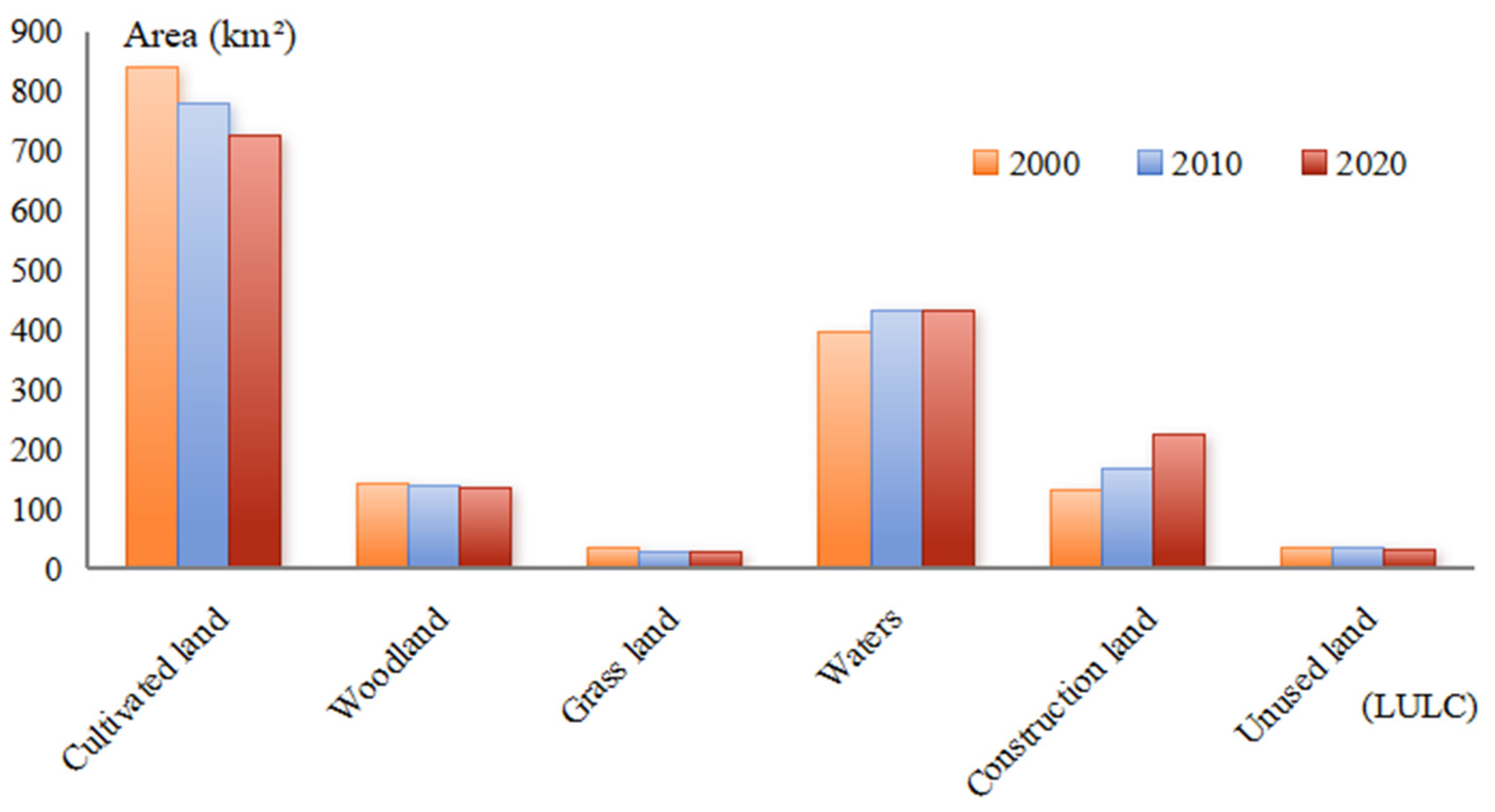
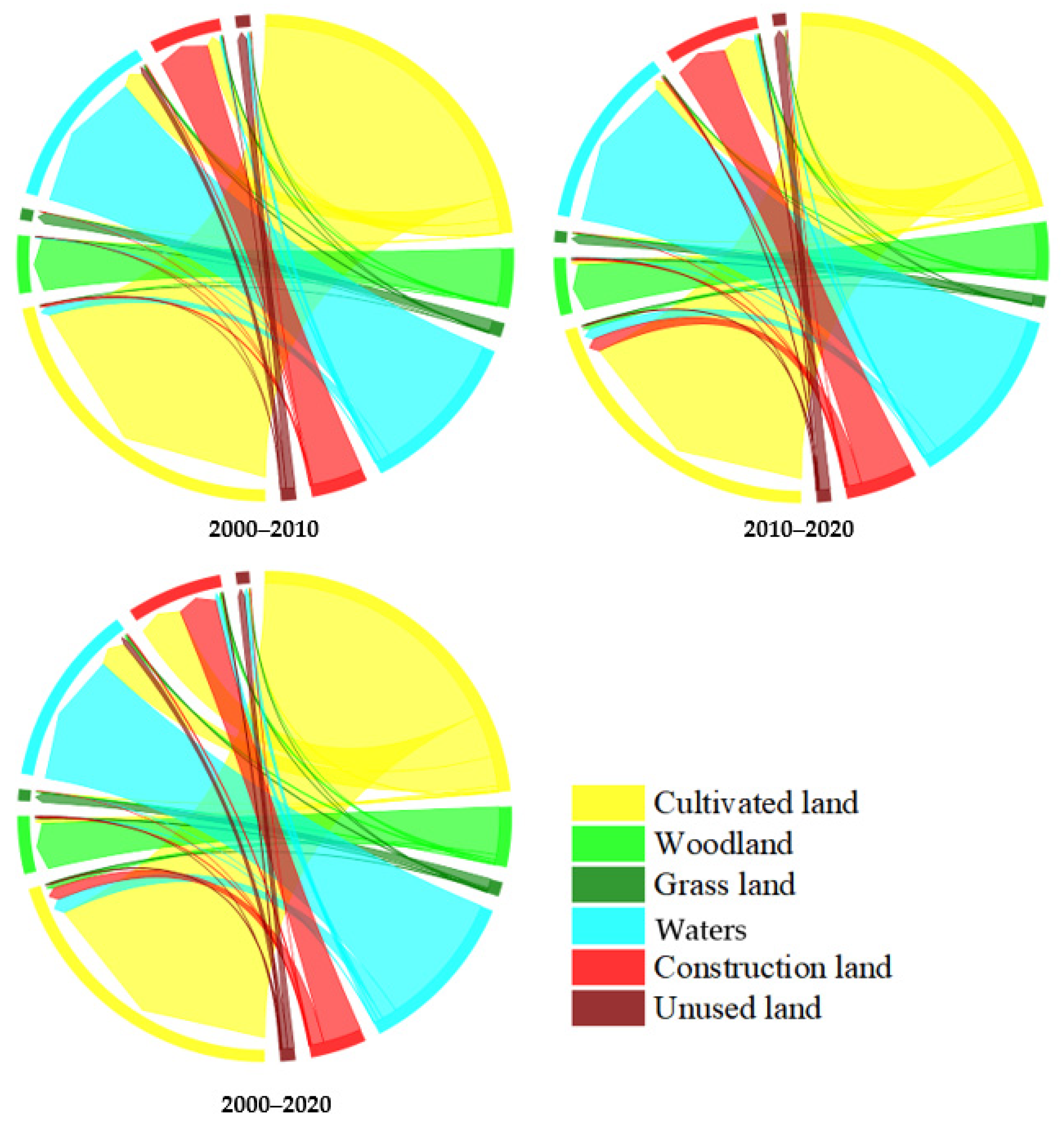
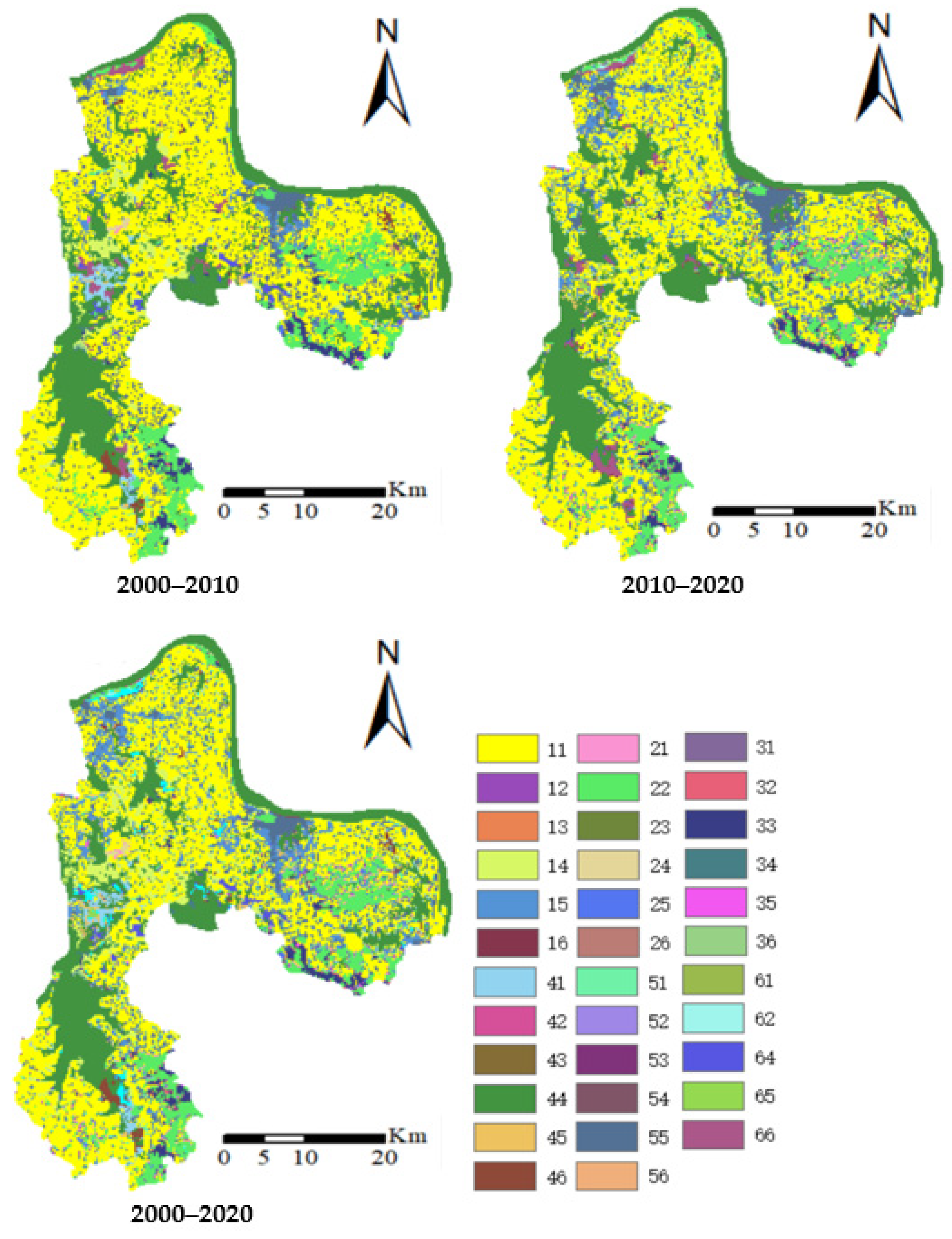
4.1. Characteristics of LULC Change

The construction land in Ezhou has continued to expand, while the agricultural and ecological space has accelerated contraction and structural reorganization (Figure 2 and Figure 3). In terms of changes in the area of various LULC types, construction land has continued to expand during the two decades, the watershed area changed very little in the latter ten years, and all other LULC types contracted to varying degrees. The most noticeable change in the scale of LULC is urban construction land, with an additional area of 94.075 km² in the twenty years, with a continuous increase in the growth rate, and a growth rate of up to 70.99% in this land use category by 2020. The watershed area expanded to 433.322 km² from 2000 to 2010, but with a small change in the latter decade. It is similar to the results of many studies, such as those showing that the rapid expansion of urbanization and human activities, which have exacerbated the continuous spread of construction land, and other land types are occupied and constrained to varying degrees [53,58,61,62,63]. This may be due to the large-scale projects implemented in the previous decade regarding river and lake restoration measures in the Yangtze River Basin, such as the return of previously reclaimed farmland to the lakes. The areas of cultivated land, woodland, grassland, and unutilized land all showed a decreasing trend during the two decades. Grassland and cropland areas contracted most significantly between 2000 and 2010, with their rates of decline being 17.10% and 7.40%, respectively. The cultivated land area continued to decline significantly in the latter decade, and the contraction rate of the cultivated land area was 6.57% in 2020. In addition, the rate of decline of woodland, grassland, and water areas from 2010 to 2020 slowed down compared with the previous decade. It shows that the industrialization on the sides of the Yangtze River and Changgang River encroaches on woodland and grassland while optimizing the ecological structure due to the implementation of ecological restoration projects.

The change of LULC types in Ezhou is characterized by the encroachment of urban space into agricultural and ecological space and the interchange of agricultural space with ecological space. Figure 4 shows the cross-shifting process of specific land use types in three periods. It reveals that the scale of conversion of farmland to waters and construction land made up more than 97% of the scale of transferring cropland out of the city from 2000 to 2010. In addition, the larger transfer areas are water bodies and construction land, with nearly 28 km² of these two land types transferred to cropland. From 2010 to 2020, the transfer of cropland to waters and construction land was still the largest, with transfer areas of 29.112 km² and 82.716 km², respectively. A greater proportion of construction land, waters, and woodland were converted to cropland during the period, accounting for 43.92%, 36.55%, and 14.04% of the area converted to cultivated land, respectively.

4.2. Multi-Scenario Land Use Change in 2030

The land use types in Ezhou are mainly characterized by cropland, watershed, and construction land in 2020, and their areas are 727.85 km², 433.32 km², and 226.59 km², respectively. The simulation results (Figure 5 and

Table 3. The area of current LULC and simulated LULC (unit: km²).

Scenarios	Current LULC (2020)	Inertial Development Scenario (2030)	Cultivated Land Protection Scenario (2030)	Ecological Priority Scenario (2030)
Cultivated land	727.85	668.21	731.88	659.84
Woodland	137.16	125.87	127.73	159.43
Grassland	27.74	25.66	25.80	33.48
Waters	433.32	420.96	431.79	446.89
Construction land	226.59	313.39	237.66	253.59
Unused land	32.29	30.85	31.09	31.72

) show that the land use characteristics of Ezhou are stable, and these three types of LULCs are still the dominant land use types in the three simulation scenarios in 2030. The changes in each type are concentrated in cropland, woodland, and construction land, with the expansion of construction land being the most significant. This may be due to the high expansion capacity of construction land as a result of the impact of human activities, especially rapid urbanization. Under the inertial development scenario, the construction land reaches 313.39 km²; as a consequence, its scale grows by 38.30% when compared to the year 2020. The area of construction land is 237.66 km², which is an increment of 4.89% compared to 2020 under the farmland protection scenario. The scale of construction land is 253.59 km², an increase of 10.13% compared to 2020 when considering the ecological priority scenario. However, the overall distribution of the LULC types remains essentially the same, when we compare the spatial distribution of LULC under different scenarios. Cropland is mainly clustered in the flat and well-developed plains in the southwestern part of the city. Forested land is mainly located in the hilly and mountainous areas of the higher terrain in the southeast, and construction land is mainly located on both sides of the rivers, mainly around the Yangtze River and the Changgang River.

4.3. Multiple Scenarios: Simulation Results of Land Use

4.3.1. Inertial Development Scenario

The inertial development scenario provides a unique perspective when exploring the many possibilities for land use change [37]. This scenario focuses on land use dynamics driven by a combination of natural and human factors in addition to policy factors [41]. Through this setting, we are able to observe more clearly the direct and far-reaching impacts of human activities on land use [52]. According to the simulation results, we can clearly see that the area of arable land is showing an obvious decreasing trend, with a specific value of 668.21 km², which is a decrease of 8.19% compared with 2020. The area of forest land and grassland is also shrinking, decreasing by 8.24% and 7.50%, respectively. This trend reflects the risk of these land types being replaced by other uses in the absence of policy guidance. What is of particular concern is the significant expansion of construction land. Its rise is as high as 38.31%, indicating that human demand for land for construction is growing rapidly to fulfill the demands of rising urbanization under this scenario [50]. This growth in demand comes mainly from the conversion of cropland, forest land, grassland, and unutilized land, making these land types the main source of construction land expansion [53]. In terms of spatial pattern, the expansion of construction land is not disorderly. It more often continues to extend along the river banks on the basis of its original distribution [54]. This expansion pattern not only occupies a large number of land categories with ecological functions, such as waters, cropland, and forest land but also reveals the profound intervention of anthropogenic actions in the physical habitat. However, the consequences of this unconstrained development pattern, if it continues, will be unimaginable [38]. The ecological environment of the region may suffer serious damage, and the reduction of natural resources such as watersheds and woodlands will directly affect the stability and function of ES.

4.3.2. Cultivated Land Protection Scenario

In the scenario of farmland protection, in order to strictly implement farmland protection, the transfer of farmland to other LULC types is restricted [52,54]. In this scenario, the cultivated land area is 731.88 km², which represents an increment of 0.55% compared to 2020. Compared to other scenarios, the farmland area has achieved a slight growth. The reduction in woodland and grassland area compared to 2020 has exceeded 6.88%, and the increase in the area of these two types has slightly decreased compared to the inertial development scenario. The expansion of construction land is significantly weaker than in the inertial development scenario, but the growth still amounted to 4.89% compared to the situation in 2020. It reveals that during the protection of farmland, the spread of construction land will be limited to a certain extent while ensuring the area of woodland and grassland. In addition, the unused land in the region has shown a downward trend compared to 2020, with an area reduction of 3.73%. Overall, this scenario slows down the rate of arable land conversion while incorporating basic farmland protection zone limiting factors and increasing conversion costs, which can effectively ensure the quantity of arable land and implement arable land protection policies [41]. However, the sprawl trend of construction land is still unavoidable due to the continuation of urbanization in the scenario, and the area of forestland, grassland, and water area has been compressed, and its encroachment on other land categories has been effectively controlled [54,55].

4.3.3. Ecological Priority Scenario

In response to the policy of “not engaging in large-scale development, but jointly focusing on large-scale protection”, an ecological priority scenario was set up [38]. The prediction results suggest that the scenario can effectively protect ecological lands including forests, grasslands, and watersheds. Compared to 2020, the woodland area of Ezhou in 2030 was 159.43 km², implying a significant upward trend, with an increase of 16.24%. Correspondingly, the grassland area was 33.48 km², an increase of 20.66%, and the waters area was 446.89 km², an increase of 3.13%. In this scenario, the significant changes in LULC are still concentrated in cropland and construction land. Compared to 2020, cropland shows a decreasing trend, and its area is further compressed by 9.34%, with an area of only 659.84 km². The sprawl of construction land is very noticeable, but its expansion rate has been effectively controlled, reducing from 38.31% in the inertial development scenario to 11.92%. In order to ensure the ecological use of land while maintaining the demand for social and economic activities, the main direction of farmland transformation is still construction land [52]. Under the ecological priority scenario, there is a growth trend in ecological land including woodland, water bodies, and grasslands, which promotes cropland to become the main type of land transfer [56]. The reduction of ecological land occupation by construction land plays a certain role in preserving ecological security.

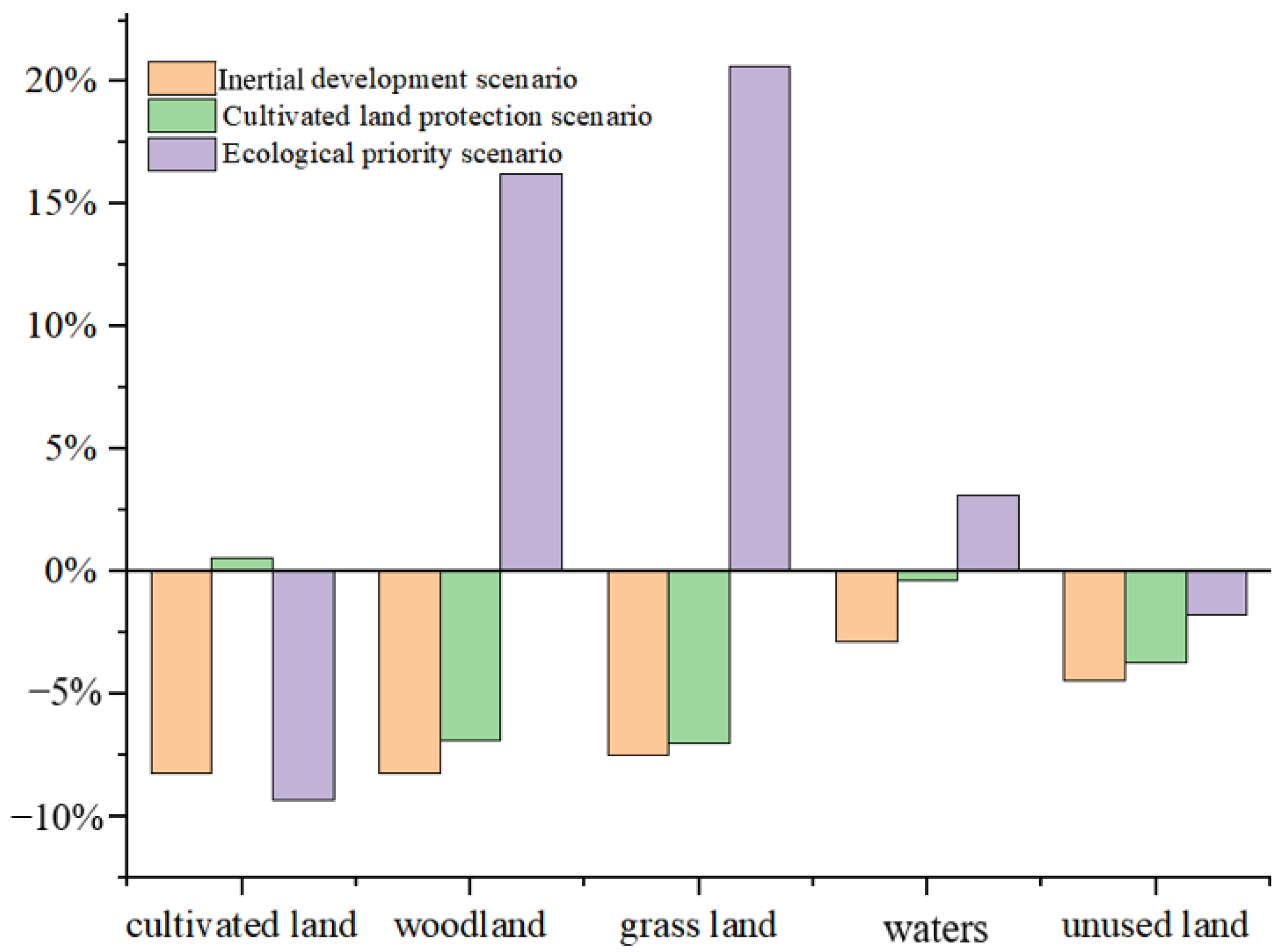
4.3.4. Comparative Analysis of LULC of Multiple Scenarios

Under the scenario of inertial development, the transfer rate of LULC remains consistent with the transfer rate from 2000 to 2020. In the absence of restrictions, the rapid expansion of construction areas and the encroachment of space for other types of land development will undoubtedly result in an increase in threats to ecological security, which will inevitably be detrimental to sustainable socio-economic development [52,54]. In addition, there are certain food security risks due to the decline in the number of croplands. Compared to other scenarios, in the scenario of farmland protection, the area of farmland has achieved effective growth, farmland has been protected to a certain extent, and the rate of outward expansion of construction land has been greatly controlled. Woodland and grassland have become the main types of transfer out, which will undoubtedly lead to a further squeeze on ecological land. Under the ecological priority scenario, the areas of woodland, grassland, and waters have all increased, and the transformation of other land types has also been regulated to varying degrees. The main manifestation is that the expansion of construction land has further decreased, from 38.31% under the inertial development scenario to about 12%. In addition, unused land maintained a downward trend in all three scenarios and was one of the sources of transfer from other land types, but its reduction was relatively lowest in the ecological protection scenario (1.76%). This is basically consistent with the findings of Wu and Athukorala et al. [51,64]. The continuous expansion of construction land will inevitably occupy a large amount of arable land, forested land, and wetlands, which is not conducive to the sustainable development of urban economy and ecology. Therefore, no matter what development scenario we choose, human beings need more space for their activities due to the advancement of urbanization and continuous socio-economic development, which directly reflects the unstoppable expansion and spreading characteristics of construction land. However, if land for construction in urban planning continues to be unrestricted by any measures, it will inevitably have a serious impact on the sustainable land use structure, damage the regional ecology, and make it difficult to achieve the development goal of ecological social economic harmony and stability. Modeling the changing needs of LULC can lead to regulatory outcomes for different land types depending on the scenarios. Regions need to comprehensively compare simulation results and further adjust unreasonable land use structures in conjunction with development goals to achieve sustainable regional development.

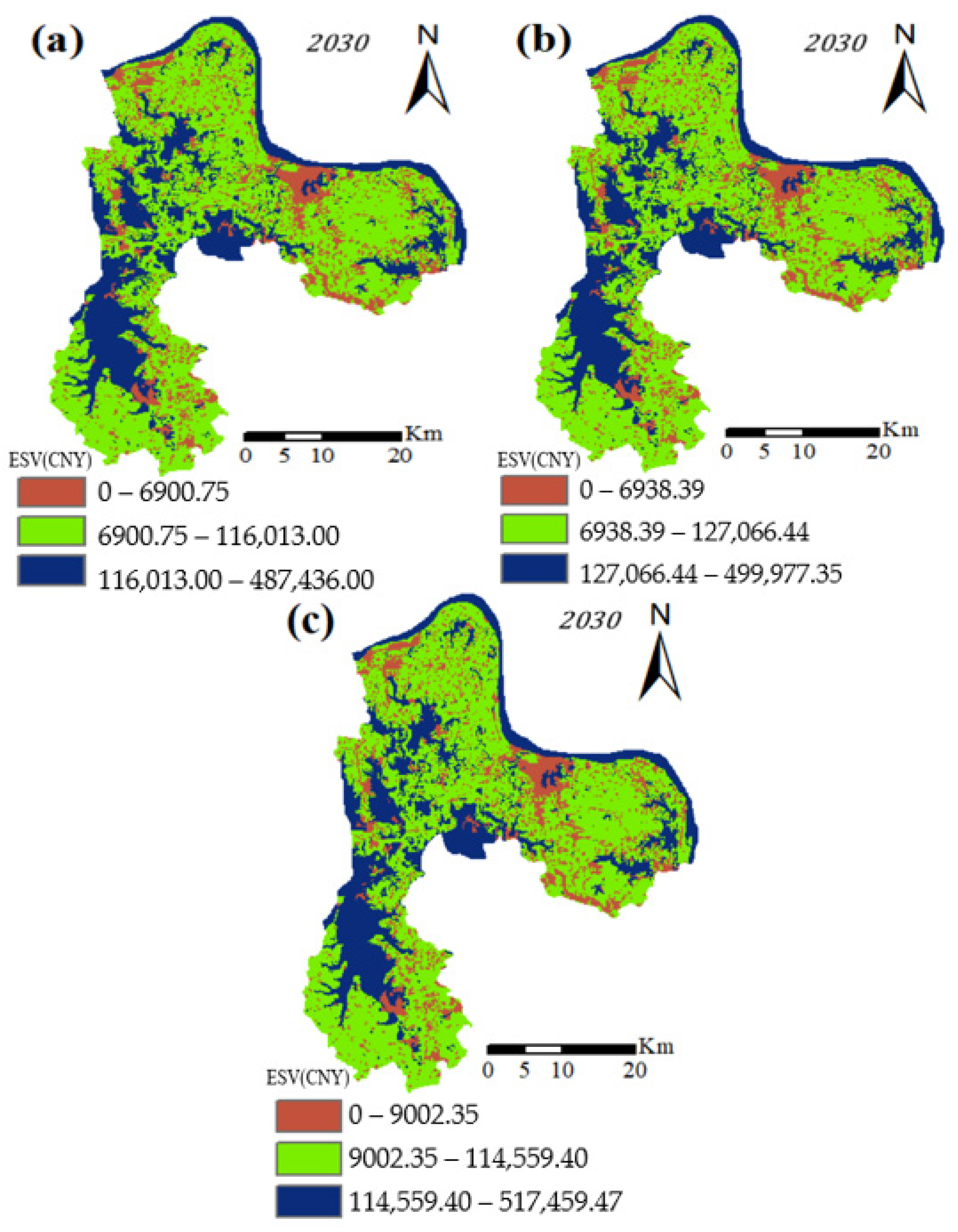
4.4. Characteristics of ESV under Multi Scenario Simulation

The total ESV of Ezhou in 2030 under the inertial development scenario, cultivated land protection scenario, and ecological priority scenario were USD 95,562.19, USD 98,987.67, and USD 102,808.99, respectively. The spatial distribution of the total ESV of Ezhou in 2030 was categorized into three categories using the natural breakpoint method in AcrGIS v10.2, as shown in Figure 6. Figure 7 shows the rate of change in ESV for the three scenarios in 2030 compared to 2020. Specifically, the 2030 ESV losses for the inertial development scenario and the farmland protection scenario are USD 4497.71 and USD 1072.23, respectively. In the case of inertial development, the high loss of ESVs can offer a decision-making foundation for future urban land planning by the government of Ezhou. Urban development cannot blindly pursue economic development, and the synergy between ecology and development is an effective method for the healthy development of the city. The ESV loss value of the farmland protection scenario is only second to the inertial development scenario, indicating that the development pattern from 2000 to 2020 is not appropriate for the current development of Ezhou. Timely adjustment of urban development strategies and optimization of urban land use layout are needed in the planning of Ezhou. However, the ESV increased by USD 2749.09 in the ecological priority scenario, indicating that the development of Ezhou needs to emphasize the conservation of the ecological land. The ecosystem services under this development scenario have great potential for improvement.

Figure 8 shows the change in ESV for individual ecosystem services in 2030 compared to 2020 for the three development scenarios in Ezhou. There are losses in each individual ESV under the inertial development scenario and farmland protection development scenario in 2030. The inertial development scenario has higher loss rates for all ESVs than the other scenarios. The highest ESV loss is in raw material production services, with a loss rate of 7.38%. The lowest ESV loss is in hydrological regulation services, with a loss rate of 3.75%. The ESV losses of various ecological services under the scenario of farmland protection and development are relatively low. Except for the high ESV losses of raw material production and gas regulation, which are 3.34% and 2.250% respectively, the ESV loss rate of other ecological services does not exceed 1%. What attracted our attention was that the ESV for food production in 2030 is USD 2704.30 under the ecological priority scenario. Compared to 2020, the rate of ESV loss is 4.94%. However, the ESV for each of the remaining ecological services shows a small increase. Under the ecological priority scenario, the ESV of supply services shows a positive increase, with an increase of USD 872.69 in hydrological regulation, USD 478.82 in waste treatment, and USD 455.30 in climate regulation. Due to the purposeful protection of the ecological space implemented in this scenario, the spread of construction land has been delayed to some extent, and the total value of ESV has increased by USD 455.30 compared to 2020. This has similarities with the findings of Schirpke, Aziz, and Raviv et al., in which the highest value of ecosystem services was found in ecological priority scenarios, which further supports the importance of protecting ecological land [7,65,66]. The protection of ecosystems such as green spaces, water bodies, and wetlands must be strengthened to support long-term economically, socially, and environmentally sustainable development.

4.5. Differences in Influence of LULC on ESV under Multiple Scenarios

Loss of watershed area, cropland, and woodland is a key factor causing changes in the ESV within the three scenarios. The reduction in ESV as a result of the reduction of waters, farmland, and woodland accounts for 43.86%, 31.72%, and 22.57% of the total value decrease in the inertial development scenario. In contrast, the reduction in ESV caused by the reduction of woodland under the scenario of farmland protection accounts for 79.04% of the total ESV reduction. Compared to these two scenarios, the overall ESV under the ecological protection scenario shows an increasing trend. Additionally, the total ESV increased by USD 2749.09 compared to 2020. Among them, the waters and woodland areas have the highest contribution rates, with their ESV growth accounting for 78.77% and 72.79% of the total ESV increase, respectively. It is generally consistent with the findings of Schirpke, Zhang, and Gashaw et al. that the decline in the area of watersheds, woodlands, and agricultural lands in the multi-scenario modeling contributed significantly to the decline in ESV [7,39,67]. This may be due to the reduced probability of converting woodland, arable land, grassland, and waters into construction land under this development scenario. In addition, due to strict restrictions such as ecological red lines, the areas of grasslands, forests, and water bodies have shown a clear enlargement, and the increase in the value of the three types of land has to some extent weakened the decrease in ESV caused by the decrease in cultivated and unused land areas. The significant increase in the area of natural landscapes (grasslands, waters, and forests) has become a huge driving force for the reduction and increase of ecosystem service value under the scenarios of cultivated land protection and ecological protection development.

5. Discussion

5.1. Land Use Change and the Ecosystem Service Value

The regional distribution of ecosystem service value (ESV) in Ezhou shows obvious characteristics, and there is a close connection between it and land use types. In these areas with high ESV values, we can see that natural land use types such as woodland, grassland, and water dominate. These areas usually have high biodiversity and provide important ecological services to the city, such as purifying air, regulating climate, and maintaining soil and water. The existence of these natural land use types plays an irreplaceable role in maintaining ecological balance and improving the quality of life of residents. However, in sharp contrast, land use types in low ESV areas are mainly construction land, including residential, commercial, and industrial land. The higher development intensity in these areas is often accompanied by a reduction in ecosystem service functions. Natural land use types such as forest land, grassland, and water bodies are rare in these areas, resulting in relatively low ecological service values. To a certain extent, this phenomenon reflects a problem in current land use planning; namely, over-emphasis on economic development at the expense of ecological protection. This phenomenon is consistent with the findings of Li, Cai, and Abd et al., who found that land use change is an important factor affecting ecological quality [8,68,69]. When land is transformed from its natural state to construction land, it tends to bring about a series of negative impacts such as the reduction of biodiversity and the decline of ecosystem service functions. This further confirms that if only ecological protection or arable land protection is focused on and the needs of economic development are ignored, then such a single development strategy is not conducive to achieving sustainable economic, social, and ecological development [70,71].

5.2. Multi-Scenario Land Use Structure and Sustainable Urban Development

Land use structure plays a crucial role in sustainable urban development, especially when facing different development scenarios. It is an indispensable basic element in the layout of urban planning and implementation and has a far-reaching impact on realizing the balanced development of urban economy, society, and ecology [56,72,73]. For Ezhou, how to guarantee the sustainability of socio-economic–urban development while ensuring that ecological livability is not threatened and realizing the harmony of economic development is an urgent problem. There is an immediate need to take into account how to rationalize the planning of future construction land, and how to regulate important food-producing land, such as cropland, and ecological land, including forests and watersheds [74,75]. Land use modeling is a complicated and dynamic process that requires consideration of numerous integrated factors, and analysis based on historical utilization does not adequately elucidate the various land use changes [76]. The evolution mechanism of the type also lacks consideration for multiple development goals, and land use prediction in multiple scenarios can provide supplementary analysis for the historical status of land use and can optimize different patterns of LULC changes according to different scenarios such as farmland protection and ecological restoration [77,78,79]. Land use prediction under multiple scenarios can provide a richer perspective for understanding the historical state of land use and optimize the pattern of land use/land cover (LULC) change according to different development scenarios, such as cropland protection and ecological restoration [80,81]. This approach has an important reference value for regional land management and land conservation and can help regional decision-makers to develop more scientific and rational land use plans and decisions and make up for the planning deficiencies that rely only on the analysis of the current situation [82].

5.3. Land Use Recommendations

Ezhou City needs to re-examine and adjust the relationship between development and protection in land use planning and management [83]. On the one hand, it is necessary to optimize the land use pattern, rationally layout various land use types, and ensure that the natural land use types are effectively protected and reasonably utilized [84,85,86]. On the other hand, it is necessary to pay attention to the overall development and protection of the country’s land space and formulate a comprehensive land use strategy in order to realize the coordinated development of ecology, economy, and society [87]. In the future specific land use process, the policy of protecting arable land should be further implemented, the illegal occupation of arable land for non-agricultural construction should be strictly prohibited, and the application conditions for the conversion of agricultural land should be strictly controlled [62,88,89,90]. In addition, ecosystem areas such as urban green spaces, wetlands, and natural landscapes play a crucial role in maintaining the ecological balance of cities. They provide a range of services, including air purification, water filtration, climate regulation, and biodiversity conservation [91,92]. The government has continued to step up its efforts to investigate and regulate the occupation of arable land and the destruction of ecological land for urban construction, while being vigilant about the occupation of arable land and the encroachment of rural settlements on areas such as green spaces, water bodies, and wetlands [93]. The land and environmental protection departments should strictly prohibit the occupation of arable land for the construction of economic forests and implement arable land restoration projects and ecological protection projects [94,95]. The planning department is gradually implementing comprehensive land improvement throughout the region to increase the area of arable land and improve the quality of the ecological environment.

5.4. Limitations and Perspectives

The modeling results of the Markov–FLUS model are closely linked to numerous factors. The selection of driving factors is easily influenced by subjectivity and limited data acquisition, coupled with the susceptibility of urban land use change to policy planning guidance, resulting in increased uncertainty in simulation results [52,96]. Although the study comprehensively considered natural and human factors, as well as policy constraints, insufficient consideration was given to factors such as the geological environment, which will be further incorporated into the model in future research [63,97]. In addition, the setting of model parameters may have some degree of subjectivity in this study [98,99]. It is mainly based on the degree of human influence on the land type and refers to previous research experience on its continuous debugging so as to reach a good simulation state. However, it does not necessarily mean accurate and perfect parameter settings. In future studies, researchers will need to continually update and rationalize the drivers of the study area [100,101,102]. This includes spatializing data on important human factors, such as regional policies, to more accurately reflect the impact of these factors on land use change [103]. Meanwhile, researchers need to consider the comprehensiveness of the driving factors, including multiple dimensions such as economic, social, and environmental, to ensure that the model can comprehensively capture the various factors affecting land use change [104,105]. In addition, the scenario settings are continuously improved and optimized according to the latest land use planning and policy directions to enhance the adaptability and foresight of the model [106].

6. Conclusions

In this study, the Markov–FLUS model was used to simulate the multi-scenario land use changes of 2030 based on LULC and other socio-economic data of Ezhou in 2000, 2010, and 2020. We calculated the ecosystem service values under different scenarios based on the multi-scenario land use and analyzed the spatial characteristics of land use change and ecosystem service values and their responses. This study can draw the following main conclusions. First, the construction land in Ezhou continues to expand from 2000 to 2020, and the other types have different levels of contraction. The growth rate of construction land to area was as high as 70.99% in 2020, and the waters area expanded to 433.322 km² from 2000 to 2010, but the change was small in the latter decade. Next, under the three scenarios, there are significant differences in the structure of land use demand. In the inertial development scenario, the area of construction land is projected to increase by 38.30% in 2030 compared to 2020. Under the farmland protection scenario, the area of construction land is 237.66 km², which represents a 4.89% increase from 2020. In contrast, under the ecological priority scenario, the scale of construction land is projected to increase by 10.13%. Furthermore, the ESVs are USD 95,562.18, USD 98,987.67, and USD 102,808.99, respectively, under the three scenarios in 2030. Compared to 2020, the ESV increased by USD 2749.09 under the ecological protection scenario. Finally, there are losses in each individual ESV under the three scenarios in 2030. The highest ESV loss is in raw material production services, with a loss rate of 7.38%. The lowest ESV loss is in hydrological regulation services, with a loss rate of 3.75%.

References

1. Smale, D.A.; Wernberg, T.; Oliver, E.C.; Thomsen, M.; Harvey, B.P.; Straub, S.C.; Straub, S.C.; Burrows, M.T.; Alexander, L.V.; Benthuysen, J.A.; et al. Marine heatwaves threaten global bio-diversity and the provision of ecosystem services. Nat. Clim. Chang. 2019, 9, 306–312. [Google Scholar] [CrossRef]
2. Zhang, M.; Tan, S.; Chen, E.; Li, J. Spatio-temporal characteristics and influencing factors of land disputes in China: Do socio-economic factors matter? Ecol. Indic. 2024, 160, 111938. [Google Scholar] [CrossRef]
3. Hu, C.; Wang, Z.; Wang, Y.; Sun, D.; Zhang, J. Combining MSPA-MCR Model to Evaluate the Ecological Network in Wuhan, China. Land 2022, 11, 213. [Google Scholar] [CrossRef]
4. Langemeyer, J.; Connolly, J.J.T. Weaving notions of justice into urban ecosystem services research and practice. Environ. Sci. Policy 2020, 109, 1–14. [Google Scholar] [CrossRef]
5. Yang, S.; Zhao, W.; Liu, Y.; Cherubini, F.; Fu, B.; Pereira, P. Prioritizing sustainable development goals and linking them to ecosystem services: A global expert’s knowledge evaluation. Geogr. Sustain. 2020, 1, 321–330. [Google Scholar] [CrossRef]
6. Lajoie-O’Malley, A.; Bronson, K.; van der Burg, S.; Klerkx, L. The future(s) of digital agriculture and sustainable food systems: An analysis of high-level policy documents. Ecosyst. Serv. 2020, 45, 101183. [Google Scholar] [CrossRef]
7. Schirpke, U.; Tscholl, S.; Tasser, E. Spatio-Temporal Changes in Ecosystem Service Values: Effects of Land-Use Changes from Past to Future (1860–2100). J. Environ. Manag. 2020, 272, 111068. [Google Scholar] [CrossRef] [PubMed]
8. Li, B.; Yang, Z.; Cai, Y.; Xie, Y.; Guo, H.; Wang, Y.; Zhang, P.; Li, B.; Jia, Q.; Huang, Y.; et al. Prediction and Valuation of Ecosystem Service Based on Land Use/Land Cover Change: A Case Study of the Pearl River Delta. Ecol. Eng. 2022, 179, 106612. [Google Scholar] [CrossRef]
9. Zhang, M.; Tan, S.; Zhang, C.; Han, S.; Zou, S.; Chen, E. Assessing the impact of fractional vegetation cover on urban thermal environment: A case study of Hangzhou, China. Sustain. Cities Soc. 2023, 96, 104663. [Google Scholar] [CrossRef]
10. Fang, Z.; Ding, T.; Chen, J.; Xue, S.; Zhou, Q.; Wang, Y.; Wang, Y.; Huang, Z.; Yang, S. Impacts of Land Use/Land Cover Changes on Ecosystem Services in Ecologically Fragile Regions. Sci. Total Environ. 2022, 831, 154967. [Google Scholar] [CrossRef]
11. Liu, L.; Zhang, H.; Zhang, Y.; Li, F.; Chen, X.; Wang, Y.; Wang, Y. Spatiotemporal heterogeneity correction in land ecosystem services and its value assessment: A case study of the Loess Plateau of China. Environ. Sci. Pollut. Res. 2023, 30, 47561–47579. [Google Scholar] [CrossRef]
12. Luo, Z.; Chen, X.; Li, N.; Li, J.; Zhang, W.; Wang, T. Spatiotemporal foresting of soil erosion for SSP-RCP scenarios considering local vegetation restoration project: A case study in the three gorges reservoir (TGR) area, China. J. Environ. Manag. 2023, 337, 117717. [Google Scholar] [CrossRef]
13. Su, Y.; Ma, X.; Feng, Q.; Liu, W.; Zhu, M.; Niu, J.; Liu, G.; Shi, L. Patterns and Controls of Ecosystem Service Values under Different Land-Use Change Scenarios in a Mining-Dominated Basin of Northern China. Ecol. Indic. 2023, 151, 110321. [Google Scholar] [CrossRef]
14. Liang, J.; Zhang, M.; Yin, Z.; Niu, K.; Li, Y.; Zhi, K.; Huang, S.; Yang, J.; Xu, M. Tripartite evolutionary game analysis and simulation research on zero-carbon production supervision of marine ranching against a carbon-neutral background. Front. Ecol. Evol. 2023, 11, 1119048. [Google Scholar] [CrossRef]
15. Ran, P.; Frazier, A.E.; Xia, C.; Tiando, D.S.; Feng, Y. How does urban landscape pattern affect ecosystem health? Insights from a spatiotemporal analysis of 212 major cities in China. Sustain. Cities Soc. 2023, 99, 104963. [Google Scholar] [CrossRef]
16. Shao, Y.; Xiao, Y.; Kou, X.; Sang, W. Sustainable land use scenarios generated by optimizing ecosystem distribution based on temporal and spatial patterns of ecosystem services in the southern China hilly region. Ecol. Inform. 2023, 78, 102275. [Google Scholar] [CrossRef]
17. Zhang, M.; Tan, S.; Zhang, C.; Chen, E. Machine learning in modelling the urban thermal field variance index and assessing the impacts of urban land expansion on seasonal thermal environment. Sustain. Cities Soc. 2024, 106, 105345. [Google Scholar] [CrossRef]
18. Costanza, R.; D’Arge, R.; De Groot, R.; Farber, S.; Grasso, M.; Hannon, B.; Paruelo, J. The value of the world’s ecosystem services and natural capital. Nature 1997, 387, 253–260. [Google Scholar] [CrossRef]
19. Costanza, R.; de Groot, R.; Sutton, P.; van der Ploeg, S.; Anderson, S.J.; Kubiszewski, I.; Farber, S.; Turner, R.K. Changes in the Global Value of Ecosystem Services. Glob. Environ. Chang. 2014, 26, 152–158. [Google Scholar] [CrossRef]
20. Farber, S.C.; Costanza, R.; Wilson, M.A. Economic and Ecological Concepts for Valuing Ecosystem Services. Ecol. Econ. 2002, 41, 375–392. [Google Scholar] [CrossRef]
21. Xie, G.; Lu, C.; Cheng, S. Progress on the valuation of global ecosystem services. Resour. Sci. 2001, 6, 5–9. (In Chinese) [Google Scholar]
22. Xie, G.; Zhang, Y.; Lu, C.; Zheng, D.; Cheng, S. Ecosystem service value of natural grassland in China. J. Nat. Resour. 2001, 1, 47–53. (In Chinese) [Google Scholar]
23. Liu, M.; Wei, H.; Dong, X.; Wang, X.; Zhao, B.; Zhang, Y. Integrating Land Use, Ecosystem Service, and Human Well-Being: A Systematic Review. Sustainability 2022, 14, 6926. [Google Scholar] [CrossRef]
24. Angelstam, P.; Munoz-Rojas, J.; Pinto-Correia, T. Landscape concepts and approaches foster learning about ecosystem services. Landsc. Ecol. 2019, 34, 1445–1460. [Google Scholar] [CrossRef]
25. Liu, Y.; Hou, X.; Li, X.; Song, B.; Wang, C. Assessing and predicting changes in ecosystem service values based on land use/cover change in the Bohai Rim coastal zone. Ecol. Indic. 2020, 111, 106004. [Google Scholar] [CrossRef]
26. Hu, B.; Li, Z.; Wu, H.; Han, H.; Cheng, X.; Kang, F. Coupling strength of human-natural systems mediates the response of ecosystem services to land use change. J. Environ. Manag. 2023, 344, 118521. [Google Scholar] [CrossRef] [PubMed]
27. Kumar, E.; Subramani, T.; Karunanidhi, D. Integrated approach of ecosystem services for mine reclamation in a clustered mining semi-urban region of South In-dia. Urban Clim. 2022, 45, 101246. [Google Scholar] [CrossRef]
28. Liu, M.; Jia, Y.; Zhao, J.; Shen, Y.; Pei, H.; Zhang, H.; Li, Y. Revegetation projects significantly improved ecosystem service values in the agro-pastoral ecotone of northern China in recent 20 years. Sci. Total Environ. 2021, 788, 147756. [Google Scholar] [CrossRef]
29. Shao, Y.; Yuan, X.; Ma, C.; Ma, R.; Ren, Z. Quantifying the Spatial Association between Land Use Change and Ecosystem Services Value: A Case Study in Xi’an, China. Sustainability 2020, 12, 4449. [Google Scholar] [CrossRef]
30. Cardoso, A.S.; Domingos, T. Integrating food provisioning ecosystem services and foodshed relocalisation targets with edible green infrastructure planning. A case study from Lisbon city region. Sustain. Cities Soc. 2023, 96, 104643. [Google Scholar] [CrossRef]
31. Carpio, A.; Ponce-Lopez, R.; Lozano-García, D.F. Urban form, land use, land cover change and their impact on carbon emissions in the Monterrey Metropolitan area, Mexico. Urban Clim. 2021, 39, 100947. [Google Scholar] [CrossRef]
32. Kindu, M.; Schneider, T.; Teketay, D.; Knoke, T. Changes of ecosystem service values in response to land use/land cover dynamics in MunessaShashemene landscape of the Ethiopian highlands. Sci. Total Environ. 2016, 547, 137–147. [Google Scholar] [CrossRef]
33. Akhtar, M.; Zhao, Y.; Gao, G.; Gulzar, Q.; Hussain, A. Assessment of spatiotemporal variations of ecosystem service values and hotspots in a dryland: A cases-tudy in Pakistan. Land Degrad. Dev. 2022, 33, 1383–1397. [Google Scholar] [CrossRef]
34. Duan, X.; Chen, Y.; Wang, L.; Zheng, G.; Liang, T. The impact of land use and land cover changes on the landscape pattern and ecosystem service value in Sanjiangyuan region of the Qinghai-Tibet Plateau. J. Environ. Manag. 2023, 325, 116539. [Google Scholar] [CrossRef] [PubMed]
35. Koo, H.; Kleemann, J.; Fuerst, C. Impact assessment of land use changes using local knowledge for the provision of ecosystem services in northern Ghana, West Africa. Ecol. Indic. 2019, 103, 156–172. [Google Scholar] [CrossRef]
36. Zhang, X.; He, J.; Deng, Z.; Ma, J.; Chen, G.; Zhang, M.; Li, D. Comparative Changes of Influence Factors of Rural Residential Area Based on Spatial Econometric Regression Model: A Case Study of Lishan Township, Hubei Province, China. Sustainability 2018, 10, 3403. [Google Scholar] [CrossRef]
37. Shi, J.; Shi, P.; Wang, Z.; Wang, L.; Li, Y. Multi-Scenario Simulation and Driving Force Analysis of Ecosystem Service Value in Arid Areas Based on PLUS Model: A Case Study of Jiuquan City, China. Land 2023, 12, 937. [Google Scholar] [CrossRef]
38. Gao, L.; Tao, F.; Liu, R.; Wang, Z.; Leng, H.; Zhou, T. Multi-scenario simulation and ecological risk analysis of land use based on the PLUS model: A case study of Nanjing. Sustain. Cities Soc. 2022, 85, 104055. [Google Scholar] [CrossRef]
39. Zhang, Z.; Peng, J.; Xu, Z.; Wang, X.; Meersmans, J. Ecosystem services supply and demand response to urbanization: A case study of the Pearl River Delta, China. Ecosyst. Serv. 2021, 49, 101274. [Google Scholar] [CrossRef]
40. Wu, C.; Chen, B.; Huang, X.; Wei, Y.H.D. Effect of land-use change and optimization on the ecosystem service values of Jiangsu Province, China. Ecol. Indic. 2020, 117, 106507. [Google Scholar] [CrossRef]
41. Chen, D.; Li, J.; Zhou, Z.; Liu, Y.; Li, T.; Liu, J. Simulating and mapping the spatial and seasonal effects of future climate and land-use changes on ecosystem services in the Yanhe watershed, China. Environ. Sci. Pollut. Res. 2018, 25, 1115–1131. [Google Scholar] [CrossRef] [PubMed]
42. Yang, J.; Xie, B.; Zhang, D. Spatial–temporal evolution of ESV and its response to land use change in the Yellow River Basin, China. Sci. Rep. 2022, 12, 13103. [Google Scholar] [CrossRef] [PubMed]
43. Li, J.; Dong, S.; Li, Y.; Wang, Y.; Li, Z.; Li, F. Effects of land use change on ecosystem services in the China–Mongolia–Russia economic corridor. J. Clean. Prod. 2022, 360, 132175. [Google Scholar] [CrossRef]
44. Muleta, T.; Kidane, M.; Bezie, A. The effect of land use/land cover change on ecosystem services values of Jibat forest landscape, Ethiopia. GeoJournal 2021, 86, 2209–2225. [Google Scholar] [CrossRef]
45. Liu, Z.; Wang, S.; Fang, C. Spatiotemporal evolution and influencing mechanism of ecosystem service value in the Guangdong-Hong Kong-Macao Greater Bay Area. J. Geogr. Sci. 2023, 33, 1226–1244. [Google Scholar] [CrossRef]
46. Li, Y.; Liu, W.; Feng, Q.; Zhu, M.; Zhang, J.; Yang, L.; Yin, X. Spatiotemporal Dynamics and Driving Factors of Ecosystem Services Value in the Hexi Regions, Northwest China. Sustainability 2022, 14, 14164. [Google Scholar] [CrossRef]
47. Wang, A.; Zhang, M.; Ren, B.; Zhang, Y.; Kafy, A.; Li, J. Ventilation analysis of urban functional zoning based on circuit model in Guangzhou in winter, China. Urban Clim. 2023, 47, 101385. [Google Scholar] [CrossRef]
48. Xiong, K.; He, C.; Chi, Y. Research Progress on Grassland Eco-Assets and Eco-Products and Its Implications for the Enhancement of Ecosystem Service Function of Karst Desertification Control. Agronomy 2023, 13, 2394. [Google Scholar] [CrossRef]
49. Xu, C.; Huang, G.; Zhang, M. Comparative Analysis of the Seasonal Driving Factors of the Urban Heat Environment Using Machine Learning: Evidence from the Wuhan Urban Agglomeration, China, 2020. Atmosphere 2024, 15, 671. [Google Scholar] [CrossRef]
50. Briner, S.; Elkin, C.; Huber, R. Evaluating the relative impact of climate and economic changes on forest and agricultural ecosystem services in mountain regions. J. Environ. Manag. 2013, 129, 414–422. [Google Scholar] [CrossRef]
51. Xiao, J.; Zhang, Y.; Xu, H. Response of ecosystem service values to land use change, 2002–2021. Ecol. Indic. 2024, 106, 111947. [Google Scholar] [CrossRef]
52. Liang, X.; Guan, Q.; Clarke, K.C.; Liu, S.; Wang, B.; Yao, Y. Understanding the drivers of sustainable land expansion using a patch-generating land use simulation (PLUS) model: A case study in Wuhan, China. Comput. Environ. Urban Syst. 2021, 85, 101569. [Google Scholar] [CrossRef]
53. Zhang, M.; Zhang, C.; Kafy, A.A.; Tan, S. Simulating the Relationship between Land Use/Cover Change and Urban Thermal Environment Using Machine Learning Algorithms in Wuhan City, China. Land 2022, 11, 14. [Google Scholar] [CrossRef]
54. Liu, P.; Hu, Y.; Jia, W. Land use optimization research based on FLUS model and ecosystem services–setting Jinan City as an example. Urban Clim. 2021, 40, 100984. [Google Scholar] [CrossRef]
55. Lin, W.; Sun, Y.; Nijhuis, S.; Wang, Z. Scenario-based flood risk assessment for urbanizing deltas using future land-use simulation (FLUS): Guangzhou Metropolitan Area as a case study. Sci. Total Environ. 2020, 739, 139899. [Google Scholar] [CrossRef]
56. Hou, L.; Wu, F.; Xie, X. The spatial characteristics and relationships between landscape pattern and ecosystem service value along an urban-rural gradient in Xi’an city, China. Ecol. Indic. 2020, 108, 105720. [Google Scholar] [CrossRef]
57. Huan, Q.; Chen, Y.; Huan, X. A Frugal Eco-Innovation Policy? Ecological Poverty Alleviation in Contemporary China from a Perspective of Eco-Civilization Progress. Sustainability 2022, 14, 4570. [Google Scholar] [CrossRef]
58. Wang, A.; Zhang, M.; Chen, E.; Zhang, C.; Han, Y. Impact of seasonal global land surface temperature (LST) change on gross primary production (GPP) in the early 21st century. Sustain. Cities Soc. 2024, 110, 105572. [Google Scholar] [CrossRef]
59. Wang, Z.; Li, X.; Mao, Y.; Li, L.; Wang, X.; Lin, Q. Dynamic simulation of land use change and assessment of carbon storage based on climate change scenarios at the city level: A case study of Bortala, China. Ecol. Indic. 2022, 134, 108499. [Google Scholar] [CrossRef]
60. Ye, F.; Chen, Y.; Li, L.; Li, Y.; Yin, Y. Multi-criteria decision-making models for smart city ranking: Evidence from the Pearl River Delta region, China. Cities 2022, 128, 103793. [Google Scholar] [CrossRef]
61. Zhu, K.; Zhou, Q.; Cheng, Y.; Zhang, Y.; Li, T.; Yan, X.; Alimov, A.; Farmanov, E.; Dávid, L.D. Regional sustainability: Pressures and responses of tourism economy and ecological environment in the Yangtze River basin, China. Front. Ecol. Evol. 2023, 11, 1148868. [Google Scholar] [CrossRef]
62. Jin, G.; Chen, K.; Liao, T.; Zhang, L.; Najmuddin, O. Measuring ecosystem services based on government intentions for future land use in Hubei Province: Implications for sustainable landscape management. Landsc. Ecol. 2021, 36, 2025–2042. [Google Scholar] [CrossRef]
63. Vollmer, D.; Pribadi, D.O.; Remondi, F.; Rustiadi, E.; Grêt-Regamey, A. Prioritizing Ecosystem Services in Rapidly Urbanizing River Basins: A Spatial Multi-Criteria Analytic Approach. Sustain. Cities Soc. 2016, 20, 237–252. [Google Scholar] [CrossRef]
64. Athukorala, D.; Murayama, Y.; Bandara, C.M.M.; Lokupitiya, E.; Hewawasam, T.; Gunatilake, J.; Karunaratne, S. Effects of Urban Land Change on Ecosystem Service Values in the Bolgoda Wetland, Sri Lanka. Sustain. Cities Soc. 2024, 101, 105050. [Google Scholar] [CrossRef]
65. Aziz, T. Changes in Land Use and Ecosystem Services Values in Pakistan, 1950–2050. Environ. Dev. 2021, 37, 100576. [Google Scholar] [CrossRef]
66. Raviv, O.; Zemah-Shamir, S.; Izhaki, I.; Lotan, A. The Effect of Wildfire and Land-Cover Changes on the Economic Value of Ecosystem Services in Mount Carmel Biosphere Reserve, Israel. Ecosyst. Serv. 2021, 49, 101291. [Google Scholar] [CrossRef]
67. Gashaw, T.; Tulu, T.; Argaw, M.; Worqlul, A.W.; Tolessa, T.; Kindu, M. Estimating the Impacts of Land Use/Land Cover Changes on Ecosystem Service Values: The Case of the Andassa Watershed in the Upper Blue Nile Basin of Ethiopia. Ecosyst. Serv. 2018, 31, 219–228. [Google Scholar] [CrossRef]
68. Cai, Y.; Zhang, P.; Wang, Q.; Wu, Y.; Ding, Y.; Nabi, M.; Fu, C.; Wang, H.; Wang, Q. How Does Water Diversion Affect Land Use Change and Ecosystem Service: A Case Study of Baiyangdian Wetland, China. J. Environ. Manag. 2023, 344, 118558. [Google Scholar] [CrossRef]
69. Abd El-Hamid, H.T.; Toubar, M.M.; Zarzoura, F.; El-Alfy, M.A. Ecosystem Services Based on Land Use/Cover and Socio-Economic Factors in Lake Burullus, a Ramsar Site, Egypt. Remote Sens. Appl. Soc. Environ. 2023, 30, 100979. [Google Scholar]
70. Chen, B.; Jing, X.; Liu, S.; Jiang, J.; Wang, Y. Intermediate human activities maximize dryland ecosystem services in the long-term land-use change: Evidence from the Sangong River watershed, northwest China. J. Environ. Manag. 2022, 319, 115708. [Google Scholar] [CrossRef]
71. Estoque, R.C.; Murayama, Y. Landscape pattern and ecosystem service value changes: Implications for environmental sustainability planning for the rapidly urbanizing summer capital of the Philippines. Landsc. Urban Plan. 2013, 116, 60–72. [Google Scholar] [CrossRef]
72. Strassburg, B.B.N.; Iribarrem, A.; Beyer, H.L.; Cordeiro, C.L.; Crouzeilles, R.; Jakovac, C.C.; Braga, J.A.; Lacerda, E.; Latawiec, A.E.; Balmford, A. Global priority areas for ecosystem restoration. Nature 2022, 609, E7. [Google Scholar] [CrossRef]
73. Zhang, M.; Tan, S.; Liang, J.; Zhang, C.; Chen, E. Predicting the impacts of urban development on urban thermal environment using machine learning algorithms in Nanjing, China. J. Environ. Manag. 2024, 356, 120560. [Google Scholar] [CrossRef] [PubMed]
74. Lawson, M.A.E.; O’Neill, I.J.; Kujawska, M.; Gowrinadh, J.S.; Wijeyesekera, A.; Flegg, Z. Breast milk-derived human milk oligosaccharides promote Bifidobacterium interac-tions within a single ecosystem. ISME J. 2020, 14, 635–648. [Google Scholar] [CrossRef] [PubMed]
75. Sirakaya, A.; Cliquet, A.; Harris, J. Ecosystem services in cities: Towards the international legal protection of ecosystem services in urban environments. Ecosyst. Serv. 2018, 29, 205–212. [Google Scholar] [CrossRef]
76. Huang, G.; Feng, S.; Hu, C. A Study of the Spatiotemporal Evolution Patterns and Coupling Coordination between Ecosystem Service Values and Habitat Quality in Diverse Scenarios: The Case of Chengdu Metropolitan Area, China. Sustainability 2024, 16, 3741. [Google Scholar] [CrossRef]
77. Xiao, R.; Lin, M.; Fei, X.; Li, Y.; Zhang, Z.; Meng, Q. Exploring the interactive coercing relationship between urbanization and ecosystem service value in the Shanghai–Hangzhou Bay Metropolitan Region. J. Clean. Prod. 2020, 253, 119803. [Google Scholar] [CrossRef]
78. Liu, G.; Meng, F.; Huang, X.; Han, Y.; Chen, Y.; Huo, Z.; Chiaka, J.C.; Yang, Q. Forecast Urban Ecosystem Services to Track Climate Change: Combining Machine Learning and Emergy Spatial Analysis. Urban Clim. 2024, 55, 101910. [Google Scholar] [CrossRef]
79. Cai, W.; Gibbs, D.; Zhang, L.; Ferrier, G.; Cai, Y. Identifying Hotspots and Management of Critical Ecosystem Services in Rapidly Urbanizing Yangtze River Delta Region, China. J. Environ. Manag. 2017, 191, 258–267. [Google Scholar] [CrossRef]
80. Tao, Y.; Wang, H.; Ou, W.; Guo, J. A Land-Cover-Based Approach to Assessing Ecosystem Services Supply and Demand Dynamics in the Rapidly Urbanizing Yangtze River Delta Region. Land Use Policy 2018, 72, 250–258. [Google Scholar] [CrossRef]
81. Wolff, S.; Schulp, C.J.E.; Verburg, P.H. Mapping Ecosystem Services Demand: A Review of Current Research and Future Perspectives. Ecol. Indic. 2015, 55, 159–171. [Google Scholar] [CrossRef]
82. Larondelle, N.; Lauf, S. Balancing Demand and Supply of Multiple Urban Ecosystem Services on Different Spatial Scales. Ecosyst. Serv. 2016, 22, 18–31. [Google Scholar] [CrossRef]
83. Hu, C.; Wang, Z.; Huang, G.; Ding, Y. Construction, Evaluation, and Optimization of a Regional Ecological Security Pattern Based on MSPA–Circuit Theory Approach. Int. J. Environ. Res. Public Health 2022, 19, 16184. [Google Scholar] [CrossRef]
84. Wang, Y.; Ma, J. Effects of land use change on ecosystem services value in Guangxi section of the Pearl River-West River Economic Belt at the county scale. Acta Ecol. Sin. 2020, 40, 7826–7839. [Google Scholar]
85. Zhang, Z.; Xia, F.; Yang, D.; Huo, J.; Wang, G.; Chen, H. Spatiotemporal characteristics in ecosystem service value and its interaction with human activities in Xinjiang, China. Ecol. Indic. 2020, 110, 105826. [Google Scholar] [CrossRef]
86. Meyfroidt, P.; Roy Chowdhury, R.; de Bremond, A.; Ellis, E.C.; Erb, K.-H.; Filatova, T.; Garrett, R.D.; Grove, J.M.; Heinimann, A.; Kuemmerle, T.; et al. Middle-Range Theories of Land System Change. Glob. Environ. Chang. 2018, 53, 52–67. [Google Scholar] [CrossRef]
87. Hu, Z.; Yang, X.; Yang, J.; Yuan, J.; Zhang, Z. Linking landscape pattern, ecosystem service value, and human well-being in Xishuangbanna, southwest China: Insights from a coupling coordination model. Glob. Ecol. Conserv. 2021, 27, e01583. [Google Scholar] [CrossRef]
88. Wang, J.; Bretz, M.; Dewan, M.A.A.; Delavar, M.A. Machine Learning in Modelling Land-Use and Land Cover-Change (LULCC): Current Status, Challenges and Prospects. Sci. Total Environ. 2022, 822, 153559. [Google Scholar] [CrossRef] [PubMed]
89. Verburg, P.H.; van de Steeg, J.; Veldkamp, A.; Willemen, L. From Land Cover Change to Land Function Dynamics: A Major Challenge to Improve Land Characterization. J. Environ. Manag. 2009, 90, 1327–1335. [Google Scholar] [CrossRef]
90. Yin, Z.; Feng, Q.; Zhu, R.; Wang, L.; Chen, Z.; Fang, C.; Lu, R. Analysis and Prediction of the Impact of Land Use/Cover Change on Ecosystem Services Value in Gansu Province, China. Ecol. Indic. 2023, 154, 110868. [Google Scholar] [CrossRef]
91. Chen, B.; Cui, B.; Ding, X. Integration of natural resources government service system and data fusion construction: Taking Nanjing as an example. Bull. Surv. Mapp. 2020, 12, 75–78. [Google Scholar]
92. Twery, M.J.; Knopp, P.D.; Thomasma, S.A.; Rauscher, H.M.; Nute, D.E.; Potter, W.D.; Maier, F.; Wang, J.; Dass, M.; Uchiyama, H.; et al. NED-2: A decision support system for integrated forest ecosystem management. Comput. Electron. Agric. 2005, 49, 24–43. [Google Scholar] [CrossRef]
93. Gómez, R.; Aguirre, J.; Oliveros, L.; Paladines, R.; Ortiz, N.; Encalada, D.; Armenteras, D. A Participatory Approach to Economic Valuation of Ecosystem Services in Andean Amazonia: Three Country Case Studies for Policy Planning. Sustainability 2023, 15, 4788. [Google Scholar] [CrossRef]
94. Frank, S.; Fürst, C.; Koschke, L.; Makeschin, F. A Contribution towards a Transfer of the Ecosystem Service Concept to Landscape Planning Using Landscape Metrics. Ecol. Indic. 2012, 21, 30–38. [Google Scholar] [CrossRef]
95. Bagstad, K.J.; Semmens, D.J.; Waage, S.; Winthrop, R. A Comparative Assessment of Decision-Support Tools for Ecosystem Services Quantification and Valuation. Ecosyst. Serv. 2013, 5, 27–39. [Google Scholar] [CrossRef]
96. Xu, X.; Peng, Y. Ecological Compensation in Zhijiang City Based on Ecosystem Service Value and Ecological Risk. Sustainability 2023, 15, 4783. [Google Scholar] [CrossRef]
97. Zhu, Z.; Mei, Z.; Xu, X.; Feng, Y.; Ren, G. Landscape ecological risk assessment based on land use change in the Yellow River basin of Shaanxi, China. Int. J. Environ. Res. Public Health 2022, 19, 9547. [Google Scholar] [CrossRef] [PubMed]
98. Liu, H.; Wang, R.Z.; Sun, H.Y.; Cao, W.J.; Song, J.; Zhang, X.F.; Wen, L.; Zhuo, Y.; Wang, L.X.; Liu, T.J. Spatiotemporal evolution and driving forces of ecosystem service value and ecological risk in the Ulan Buh Desert. Front. Environ. Sci. 2023, 10, 2659. [Google Scholar] [CrossRef]
99. Xiong, S.G.; Wan, J.; Long, H.L.; Yu, L. Spatiotemporal dynamics and implications of ecosystem service value in the key ecological function area—Case of Yichang city, Hubei Province. Res. Soil Water Conserv. 2016, 23, 296–302. [Google Scholar]
100. Hu, S.; Chen, L.Q.; Li, L.; Wang, B.Y.; Yuan, L.N.; Cheng, L.; Yu, Z.Q.; Zhang, T. Spatiotemporal dynamics of ecosystem service value determined by land-use changes in the urbanization of Anhui Province, China. Int. J. Environ. Res. Public Health 2019, 16, 5104. [Google Scholar] [CrossRef]
101. Salzman, J.; Bennett, G.; Carroll, N.; Goldstein, A.; Jenkins, M. The Global Status and Trends of Payments for Ecosystem Services. Nat. Sustain. 2018, 1, 136–144. [Google Scholar] [CrossRef]
102. Feagin, R.A.; Martinez, M.L.; Mendoza-Gonzalez, G.; Costanza, R. Salt marsh zonal migration and ecosystem service change in response to global sea level rise: A case study from an urban region. Ecol. Soc. 2010, 15, 14. [Google Scholar] [CrossRef]
103. Lai, J.; Li, J.; Liu, L. Predicting Soil Erosion Using RUSLE and GeoSOS-FLUS Models: A Case Study in Kunming, China. Forests 2024, 15, 1039. [Google Scholar] [CrossRef]
104. Mamitimin, Y.; Simayi, Z.; Mamat, A.; Maimaiti, B.; Ma, Y. FLUS Based Modeling of the Urban LULC in Arid and Semi-Arid Region of Northwest China: A Case Study of Urumqi City. Sustainability 2023, 15, 4912. [Google Scholar] [CrossRef]
105. Ma, B.; Wang, X. What Is the Future of Ecological Space in Wuhan Metropolitan Area? A Multi-Scenario Simulation Based on Markov-Flus. Ecol. Indic. 2022, 141, 109124. [Google Scholar] [CrossRef]
106. Yang, X.; Zheng, X.-Q.; Chen, R. A Land Use Change Model: Integrating Landscape Pattern Indexes and Markov-Ca. Ecol. Model. 2014, 283, 1–7. [Google Scholar] [CrossRef]
Figure 1. Geographical Area Map (a) and Elevation Map of Ezhou (b).
Sustainability 16 06237 g001
Figure 2. Statistical map of the area of land use types.
Sustainability 16 06237 g002
Figure 3. Land use transfer chord map of Ezhou.
Sustainability 16 06237 g003
Figure 4. Map of the transfer of LULC types. Notes: Codes 1–6 indicate cropland, woodland, grassland, waters, construction land, and unused land. The mapping code is a combination of two converted secondary space codes. For example, “cropland → woodland” (code 12).
Sustainability 16 06237 g004
Figure 5. Land use change in 2030 under three scenarios; (a) for the inertial development scenario, (b) for the cultivated land protection scenario, (c) for the ecological priority scenario.
Sustainability 16 06237 g005
Figure 6. The ESV under different scenarios; (a) for the inertial development scenario, (b) for the cultivated land protection scenario, (c) for the ecological priority scenario.
Sustainability 16 06237 g006
Figure 7. The ESV change rate under different scenarios in 2030.
Sustainability 16 06237 g007
Figure 8. Changes in individual ESV in 2030 (compared to 2020).
Sustainability 16 06237 g008