Abstract
To enhance the efficient utilization of space resources, it is critical to integrate information from various systems of the space station and formulate scientific and effective methods for planning cargo supplies. Considering the large-scale, multi-objective, complex nonlinear, non-convex, non-differentiable, and mixed-integer characteristics, this study decomposes the space station cargo supply planning problem into a bi-level optimization problem involving cargo manifest and loading layout iterations. A new CILPSO algorithm is proposed to solve this by integrating particle coding, reliability priority, and random generation mechanisms of population initialization, global and local versions of particle updating, and a local search strategy. The experimental results show that the CILPSO algorithm outperforms other algorithms regarding search performance and convergence efficiency. The proposed approach can effectively reduce the cargo supply cost of the space station and improve the output of space science and application achievements. It provides a decision-making basis for the responsible department to develop cargo supply schemes, for the cargo supply systems to submit cargo demands, and for the cargo spaceship system to design loading schemes. This study advances the logistics sustainability of the space station.
1. Introduction
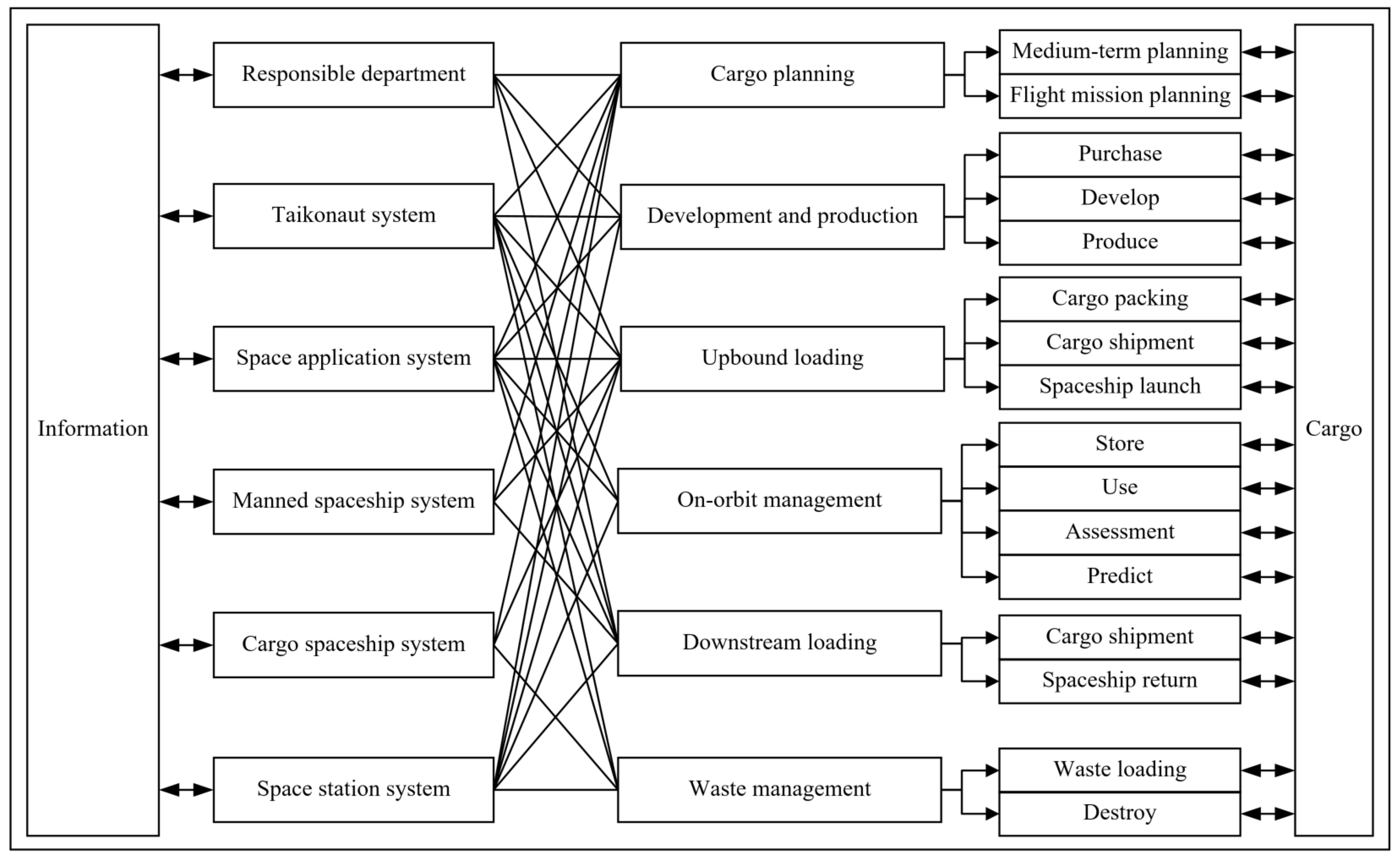
The cargo spaceship was built to construct the space station, which facilitates space applications. The ultimate goal of the China Manned Space Program is the application of space technology [1]. The China Space Station, completed at the end of 2022 and orbiting over 400 km above Earth, has entered the phase of large-scale and long-term manned operations. To ensure the safe operation of the platform and successfully conduct space science and application experiments, a large amount of cargo must be transported to the space station in a timely and accurate manner. Hence, the logistics management of the space station is crucial.
The logistics of the China Space Station are designed to maintain the health of taikonauts and maximize application achievements. It is a comprehensive lifecycle process that manages the flow of cargo to and from the station as required. Cargo planning is integral throughout this process, coordinating the needs of the taikonaut system, the space application system, and the space station system. Furthermore, it promotes the planning and management of systematic development, ascent, and descent, as well as operations. The space station supply cargo includes equipment and items launched to the space station by spaceships. Figure 1 illustrates the logistics process of the China Space Station.
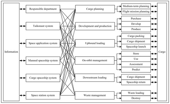
Figure 1.
Logistics process of the China Space Station.
Cargo supply planning for the space station is a crucial aspect of logistics management. Its engineering characteristics include a multi-variety and small-batch production model, robust planning, prioritization, redundant system reliability, high transportation costs, spaceship-rated loading capacity, fixed time windows, and complex coupling constraints. Academic research on space station cargo supply has focused on total cargo supply allocation, cargo manifest planning, packing problems, launch time planning, spaceship design, and route planning [2,3,4,5,6,7,8,9,10,11,12,13,14]. Current issues include insufficient collaboration among systems, information asymmetry, and incomplete consideration of factors affecting cargo supply. These issues hinder scientific and reasonable overall planning, leading to occasional oversupply of cargo. Furthermore, resource allocation—such as funds, spaceship space, and taikonaut work hours—requires optimization. Meanwhile, the efficiency of space resource utilization can be improved. Space resource utilization efficiency refers to the output-to-input ratio for space resources. Output includes space science and application achievements, whereas input relates to cargo supply costs. Therefore, proposing scientific and effective planning methods to reduce cargo supply costs and enhance space science and application outputs is imperative.
To achieve efficient resource coordination, this study proposes a cargo supply planning approach for the space station. The approach considers the entire station scenario and consolidates information from all systems. It integrates multiple cargo supply strategies and principles, considers various design variables, objectives, and constraints neglected by existing research, and constructs a mixed-integer nonlinear programming model for global optimization. However, the model exhibits large-scale, multi-objective, complex nonlinear, non-convex, non-differentiable, and mixed-integer characteristics, making it difficult to solve directly with existing methods. Therefore, the space station cargo supply planning problem is decomposed into a bi-level optimization problem, iterating between the cargo manifest and the loading layout. Additionally, an efficient CPLEX-embedded improved local-search particle swarm optimization (CILPSO) algorithm is designed to suit the problem’s characteristics.
Under the condition of ensuring engineering reliability, a scientific and effective optimization model is established for high-efficiency and low-cost planning of the China Space Station’s cargo supply. The entire cargo supply management process is optimized, improving the efficiency of space resource utilization. The model aims to minimize logistics costs, maximize space science and application achievements, and reduce space waste burning and discharging in orbit. Hence, this study promotes the sustainable development of space station logistics.
The structure of the study is outlined as follows: Section 2 introduces the current status and gaps in research and emphasizes the contributions of this study. Section 3 establishes a planning model for space station cargo supply. Section 4 proposes the CILPSO algorithm. Section 5 presents a case study on the proposed model and algorithm. Section 6 summarizes the research.
2. Related Work
This section first reviews research on general industry cargo supply planning, distinguishing the differences between the aerospace industry and the general industry. Next, it discusses the current status and gaps in research on space station cargo supply planning. It then explores research on cargo manifest optimization and loading layout optimization. Finally, it analyzes the current status and gaps of research related to the model characteristics in this study. Based on the above research, the main contributions of this study are summarized.
2.1. General Industry Cargo Supply Planning
The cargo supply planning problem is critical in the fields of retailing [15], the manufacturing industry [16,17], the medical industry [18], the military industry [19,20], disaster emergency [21,22], cold chain logistics [23], and others. General cargo supply planning methods are classified into mixed-integer linear/nonlinear programming, dynamic programming, stochastic programming, robust optimization, reinforcement learning, and multi-agent simulation. The distinguishing characteristics of space station cargo supply compared to other industries are as follows. The cargo consists of various types with small batches. Cargo supplies undergo the mid-term planning three years in advance and the flight mission planning one year in advance. The priority of cargo is divided into four levels according to the importance. The transportation costs are high, and the utilization of resources is pursued to the utmost extent. The rated loading capacity of the spaceship is limited. The spaceship launch time window is fixed. Redundant cargo supply is adopted to ensure the system’s reliability. The system is subject to many influencing factors, presenting intricate coupling constraints. General cargo supply planning methods do not account for the characteristics of space station cargo supply. Therefore, it is necessary to design a characteristic-based scientific method to plan space station cargo supply reasonably.
2.2. Space Station Cargo Supply Planning
Research related to the cargo supply planning of the China Space Station focuses on total cargo supply allocation, cargo manifest planning, packing problems, launch time planning, etc. Lin et al. [2] researched and discussed the optimization of logistics strategies for long-term space station operations, considering the visit time and the payload manifest of the coordinated flights of the cargo spaceship. They defined four metrics to quantify the utilization benefit and the operational robustness of the space station operation scenarios. Moreover, they employed a genetic algorithm to obtain the optimal solution. Later, Lin et al. [3] extended the previously proposed single-objective optimization formulation to multi-objective optimization formulations for space station logistics strategy. They adopted physical planning to transform the four-objective optimization problem into a single-objective optimization problem. Furthermore, they proposed a genetic algorithm to solve the outcome-based physical planning optimization problem. Zhu et al. [4] proposed a hybrid approach combining a multi-objective evolutionary algorithm, physical programming, and a differential evolutionary algorithm to handle the optimization and decision-making of logistics strategies for the space station.
Compared with the research related to the cargo supply planning of the China Space Station, the scenarios faced by the International Space Station (ISS) are more complex. The ISS includes multiple cargo spaceship types, considering multi-node and multi-transportation scenarios. Gralla et al. [5] proposed SpaceNet, a modeling framework for interplanetary supply chain management, to characterize and evaluate the space logistic architecture and support the modeling of crew, cargo, and spaceship flows through the Earth–Moon–Mars system. Research related to ISS cargo supply planning can be categorized into three types according to methodology:
The first category assigns commodities to elements and then elements to paths. Taylor et al. [6] developed a sustainable spatial transportation architecture. The problem consists of three components: commodities or supplies that must be transported to meet mission requirements, elements or physical structures used to store and transport the commodities, and the network or paths for transporting the elements and commodities. Taylor et al. [7] applied mixed-integer nonlinear programming to optimize spaceship design and network flows simultaneously to obtain a transportation architecture. They embedded the integer programming solver CPLEX within the perturbation step of simulated annealing to solve the numerous linear inequality and equality constraints imposed by flow feasibility and operational constraints.
The second category employs matrix-based methods to obtain the optimal cargo manifest. For single-node and multi-transportation scenarios, a “front-fill” algorithm is used to obtain the cargo manifest matrix. Siddiqi et al. [8] used a matrix-based approach to create a manifest matrix and a flight dependency matrix for ISS supply cargo. Siddiqi et al. [9] quantified how to deliver what cargo and when given future demand and consumption. They proposed the M-matrix to simplify the manifest representation of flight cargo involving numerous flights and mission activities. For multi-node and multi-transportation scenarios, a linear programming or flow network approach is used to find the minimum flow manifest as the initial manifest for optimization. To find the optimal manifest that meets the desired objective function, they employed linear or non-linear programming methods and system objective functions. Grogan et al. [10] extended from a single-node scenario to a multi-node and multi-transportation scenario, proposing a matrix-based approach for determining the optimal manifest of spatial exploration. The matrix represents the cargo carried by the means of transportation, used to satisfy the demand, and transferred to other means of transportation. Grogan et al. [11] combined the matrix-based optimal display approach with the SpaceNet model to implement a spatial logistics modeling framework in the form of a discrete-event simulation tool.
The third category designs the Integrated Space Station Optimization (ISSO) framework and proposes the corresponding optimization methodology. Ho et al. [12,13] combined the space habitat and its logistics design into an optimization problem. They used nonlinear programming and bi-objective optimization to minimize the logistics costs while maximizing science achievements. Ho et al. [14] improved the previously proposed ISSO formulation, including the definition of scientific achievements. The definition considers imbalances of multiple attributes such as payload mass and crew time rather than their simple weighted average value. They employed nonlinear programming, bi-objective optimization, and sequential quadratic programming to minimize logistics costs while maximizing science achievements.
The research mentioned above, which combined different backgrounds and needs, has conducted relevant research on cargo supply planning for both the China Space Station and the International Space Station. While these studies possess specific theoretical and practical significance, there are still the following deficiencies: (1) The influencing factors of cargo supply are not considered comprehensively. Only factors affecting cargo supply, such as cargo priority, cargo demand satisfaction, spaceship loading capacity, on-orbit inventory status, and supply time, are considered. However, factors like loading priority, taikonaut work hours, cargo grid volume of cargo spaceship, loading stability, and redundant system reliability are not considered. There is a lack of consideration of the mutual influence between various elements from the overall planning perspective, such as sharing cargo among systems to save resources. The planning results deviate from the actual needs. (2) The cargo manifest and the loading layout are not synergistically optimized. In the process of cargo supply planning, the cargo manifest is planned based only on certain factors affecting cargo supply, without considering the relevant constraints on the loading layout of the cargo spaceship. This leads to repeated manual iterations of the cargo manifest and the loading layout in actual engineering. The generated cargo supply scheme did not reach the global optimum.
2.3. Cargo Manifest Optimization
In shipping logistics and aviation logistics, scholars establish linear models or nonlinear models to solve the cargo manifest optimization problem according to its complexity. Existing research generally pursues the maximization of economic benefit through cargo selection. Additionally, some studies have considered factors such as cargo priority and environmental protection.
Bilican et al. [24] proposed mixed-integer nonlinear programming and a two-stage solution approach to solve the problem of cargo selection and stowage plan in container shipping service. In the cargo selection process, the containers in each bay are selected to maximize total revenue and minimize both over-stowage and crane emissions. Brandt et al. [25] summarized the aircraft configuration problem in the cargo load planning problem of air cargo carriers. No scholars have addressed the theoretical complexity of selecting the types and number of unit load devices (ULDs) to be built for a flight. Seixas et al. [26] studied the problem of cargo selection and stowing on the supply vessel to maximize the sum of cargo priority and overall benefit. They proposed a probabilistic constructive procedure combined with a local search heuristic to solve the variation of the two-dimensional knapsack problem. Vancroonenburg et al. [27] introduced a mixed-integer linear programming method to solve the problem of automatic air cargo selection and weight balancing, finding the optimal selection from a set of cargo to be loaded on the aircraft.
2.4. Loading Layout Optimization
There has been a lot of research on loading layout optimization in shipping and aviation logistics. Most research mainly focuses on loading position, loading stability, weight limitation, and other factors. Methods to achieve loading stability include minimizing the deviation of the center of gravity, implementing class-based stowage plans, and minimizing trimming moments, among others.
Vancroonenburg et al. [27] minimized the deviation between the aircraft’s center of gravity and the known target value, thereby improving the stability of air cargo. Iris et al. [28] solved the flexible containership loading problem by establishing a mathematical model and a heuristic algorithm. It assumes that the vessel’s stability is guaranteed by the class-based stowage plan. Brandt et al. [25] summarized the weight and balance problem in cargo load planning of air cargo carriers. When deciding the loading positions of ULDs within an aircraft, several factors need to be considered: ULD assignment, loading position allocation, overlapping positions, total weight limit, cumulative weights, center of gravity, moments of inertia, loading dependencies, ULD separation, and loading operations. Based on the cargo selection, Bilican et al. [24] realized the stability planning of the containership by minimizing the trimming moment, thereby generating a detailed slot-assignment plan. Zhou et al. [29] studied the air cargo planning problem considering shipment consolidation and containerization. They designed a biased random-key genetic algorithm combined with a three-dimensional packing heuristic to solve the mixed-integer programming model.
2.5. Research Related to Model Characteristics
The space station cargo supply planning model proposed in this study is an NP-hard problem characterized by large-scale, multi-objective, complex nonlinear, non-convex, non-differentiable, and mixed-integer properties.
Jaber et al. [30] proposed a generalized hybrid approach based on multi-criteria branch-and-bound and NSGA-II to enhance the approximate Pareto frontiers for a multi-objective mixed-integer nonlinear programming problem. Artis et al. [31] proposed a novel multi-objective non-convex mixed-integer nonlinear master–slave optimization problem for emergency-constrained transmission expansion planning. They employed a symphony orchestra search algorithm (SOSA) with multi-computational steps, as well as multi-dimensional and multi-homogeneous structures, for better diversification and exploration. Chen et al. [32] partitioned a large-scale wind farm into multiple decoupled subsets utilizing PDFS and HITS algorithms based on the directional map of the tail flow. They used a combined Monte Carlo–beetle swarm optimization (CMC-BSO) algorithm to solve a multi-objective non-convex optimization problem.
No scholars have yet proposed an efficient method to solve the complex nonlinear problem of variables in the space station cargo supply planning model, which involves product, summation, permutation, combination, and exponentiation operations.
2.6. Main Contributions
The main contributions of the study are as follows:
- We propose strategies and principles for space station cargo supply. For example, single-layer redundancy with minimum waste, high cargo priority, first-in-last-out, and loading stability.
- We integrate information resources from various systems of the space station and implement scientific and reasonable overall planning. Comprehensively integrate actual cargo demand, on-orbit inventory, reliability, and other data of various space station systems, transforming the local optimization of space station cargo supply planning into global optimization.
- We incorporate design variables that have not been considered before. For example, whether and how much cargo is supplied, and where cargo is loaded in the spaceship.
- We add unique objectives and constraints that have not been considered. For example, first-in-last-out according to mission sequencing, taikonaut work hours constraints, cargo grid volume constraints of cargo spaceship, loading stability constraints, and redundant system reliability constraints.
- We design the bi-level optimization model and the CILPSO algorithm. Based on the characteristics of the space station cargo supply planning model, the model is decomposed into a bi-level optimization problem iterated by cargo manifest and loading layout. A new CILPSO algorithm integrating particle coding, population initialization mechanisms of reliability priority and random generation, global and local versions of particle updating, and a local search strategy is proposed to solve the complex nonlinear intractable problem.
3. Modeling of Space Station Cargo Supply Planning
3.1. Problem Description
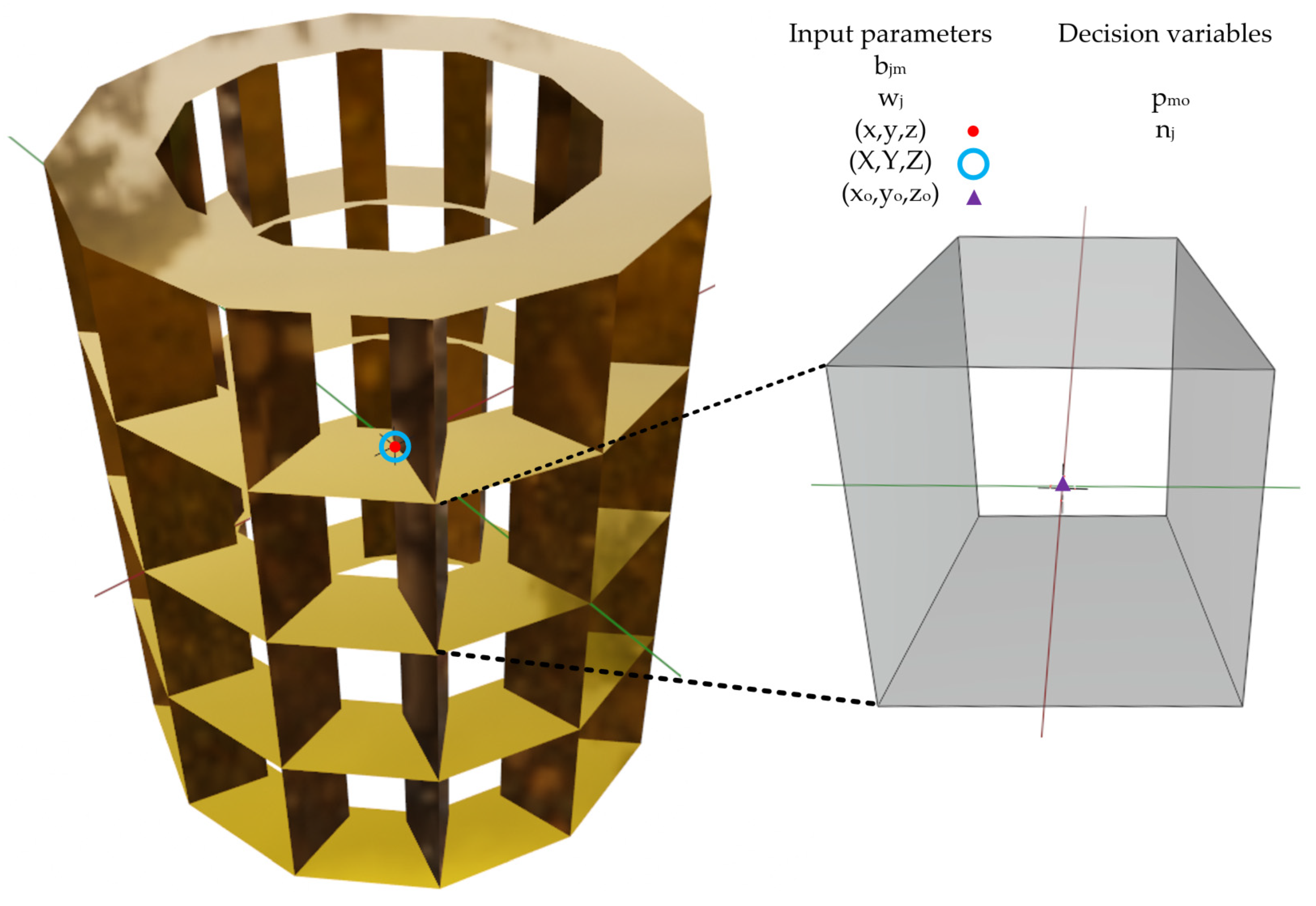
The taikonaut system, space station platform system, and space application system submit their cargo demands to the responsible department. The responsible department then considers various factors to formulate a cargo supply scheme and supply large quantities of cargo to the space station timely and accurately via the Tianzhou Cargo Spaceship. The types of upbound cargo carried by each system on board the cargo spaceship are shown in Table 1. The responsible department determines the quantity and timing of spaceship launches. The Tianzhou Cargo Spaceship is a circular cabin structure consisting of a propulsion module and a cargo module. The propulsion module carries storage tanks to replenish propellants for the space station. The cargo module features a honeycomb structure with four layers, each containing twelve cargo grids to store other cargo.

Table 1.
Types of supplies for the Cargo Spaceship.
The problem investigated in this study is to determine the type and quantity of space station cargo supply, as well as the locations of cargo on the spaceship. This decision is made by comprehensively considering the actual cargo demands of various space station systems, the amount of inventory in orbit, reliability, and other related information from the perspective of the whole life cycle of space station cargo supply. The objective functions are to minimize the cargo supply cost of the space station and maximize the output of space science and application achievements. This decision-making process is subject to a series of complex and coupled constraints: priority satisfaction of important cargo demands, first-in-last-out principle, cargo demands, loading capacity, taikonaut work hours, cargo grid volume, loading stability, cargo on-orbit inventory, and reliability of redundant systems. As a result, the cost and benefit of space station cargo supply will be balanced while fulfilling the requirements, thus minimizing the waste of space resources.
3.2. Assumption
In practical engineering, there are instances where the cargo of a single mission may need to be placed into multiple cargo grids, although such occurrences are relatively infrequent. Cargo grids on a cargo spaceship are numbered based on their coordinates, whereas missions are numbered according to different systems. These factors make the planning problem extremely complicated. To better understand the nature of the problem, it is necessary to simplify and adjust the research problem accordingly. The assumptions of this study are as follows:
- The cargo of a single mission is placed into only one cargo grid, but a single cargo grid can hold cargo from multiple missions.
- The indices of cargo grids are larger for those closer to the exit hatch of the cargo spaceship, while they are smaller for those further away from the exit hatch.
- Missions are prioritized in order of time urgency. Those with larger indices of missions are more urgent and loaded in positions closer to the exit hatch of the cargo spaceship.
3.3. Notation
For the convenience of describing the model, the notations are defined as follows:
(1) Indices and sets.
: Set of cargo types;
: Set of cargo grids on cargo spaceship;
: Set of missions.
(2) Input parameters.
: Unit cost of cargo ;
: Unit weight of cargo ;
: Loading capacity of cargo spaceship;
: Unit work hours for taikonauts handling cargo ;
: Prescribed maximum total work hours for taikonauts handling cargo;
: Whether mission is a science and application experiment or not, taking 1 for yes and 0 for no;
: Whether cargo belongs to mission or not, taking 1 for yes and 0 for no;
: Demand for cargo ;
: On-orbit inventory of cargo ;
: Unit volume of cargo ;
: Capacity of each cargo grid;
: Priority of cargo , ;
: Center of gravity position of cargo grid ;
: Center of gravity position of cargo spaceship;
: Safe floating range of cargo spaceship’s center of gravity on the axis, axis, and axis after loading;
: Reliability of cargo ;
: Objective reliability level of each mission.
(3) Decision variables
: Whether cargo is supplied or not, taking 1 for yes and 0 for no;
: Supply quantity of cargo ;
: Total supply quantity of cargo ;
: Whether mission is placed in cargo grid , taking 1 for yes and 0 for no;
: Iterative variable, the value range is from to in steps of 1.
3.4. Model Construction
The space station cargo supply planning model is expressed as follows:
, , , are large positive numbers.
Objective function (1) minimizes the total cargo supply cost for the space station. This entails minimizing the total cost of supplying cargo necessary to maintain the health of taikonauts, ensure the safe operation of the platform, and support scientific and application experiments, thereby enhancing the economic benefits of cargo supply.
Objective function (2) maximizes the total output of the space science and application achievements. This maximization strengthens the contribution to the overall welfare and operation of society. The output is proportional to two factors: the weight of the upbound payloads (denoted as ) and the work hours of taikonauts spent on scientific and experimental missions (denoted as ). Therefore, objective function (2) is nonlinear.
Objective function (3) maximizes the total sum of the priority of cargo supply, prioritizing the fulfillment of critical cargo demands.
Objective function (4) enforces the loading priority rule of first-in-last-out. It is related to the indices of missions sorted by time urgency and the indices of cargo grids sorted by proximity to the cargo spaceship’s exit hatch.
Constraints (5) and (6) establish the logical relationship between the decision variables of whether cargo is supplied and the quantity of cargo to be supplied.
Constraint (7) specifies that the total weight of upbound cargo should not exceed the loading capacity of the cargo spaceship. This reduces the burden on the space orbit from the root, limits the weight of space waste incineration emissions, and protects the space environment.
Constraint (8) ensures that the taikonaut’s work hours for handling all mission cargo do not exceed the total work hours.
Constraint (9) dictates that the total volume of cargo placed into the cargo grid cannot exceed the capacity of each cargo grid. As and are decision variables, this constraint is nonlinear.
Constraint (10) states that cargo for a single mission is placed into only one cargo grid, and a cargo grid can hold cargo from multiple missions.
Constraints (11) and (12) define the logical relationship between the decision variables of whether cargo is supplied and whether mission is placed into cargo grid .
Constraints (13)–(15) ensure that the overall center of gravity of the cargo, after loading, remains within a specified deviation range to maintain the stability of the cargo spaceship. To better understand stability constraints, Figure 2 illustrates a simple scenario of stability constraints. The left side of Figure 2 shows the position and deviation range of the cargo spaceship’s center of gravity, represented by and respectively. The right side of Figure 2 shows the center of gravity position of the cargo grid, represented by . Nonlinear stability constraints can be transformed into linear constraints using the absolute value inequality property. See Section 3.5 for the derivation process.
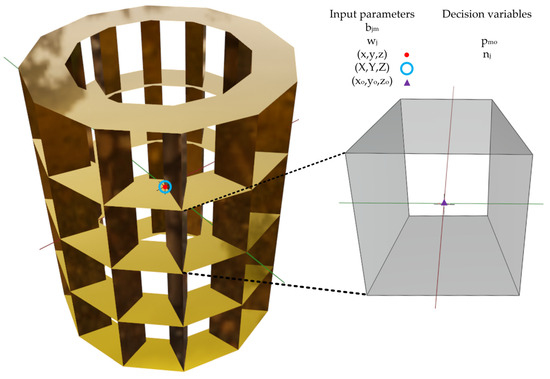
Figure 2.
Simple scenario description of stability constraints.
Constraint (16) states that the sum of the supply quantity of cargo and its on-orbit inventory equals the total supply quantity of cargo .
Constraint (17) requires that the mission reliability of the single-layer series-parallel redundancy system is not less than the objective reliability level of each mission. The decision variable of Constraint (17) appears in product, summation, permutation and combination, and exponentiation operations. Hence, Constraint (17) is a complex nonlinear constraint. Its theoretical basis lies in the reliability of series-parallel and redundant systems [33]. See Appendix A for the detailed derivation process of this constraint.
Constraints (18)–(22) denote the range of decision variables.
3.5. Stability Constraints Linearization
According to the nature of absolute value inequality, the nonlinear stability Constraint (13) is linearized into Equations (23) and (24).
Equation (13) is equivalent to Equations (23) and (24), and the derivation process is as follows.
Thus, Equations (23) and (24) are obtained. Similarly, Equation (14) is equivalent to Equations (27) and (28), and Equation (15) is equivalent to Equations (29) and (30).
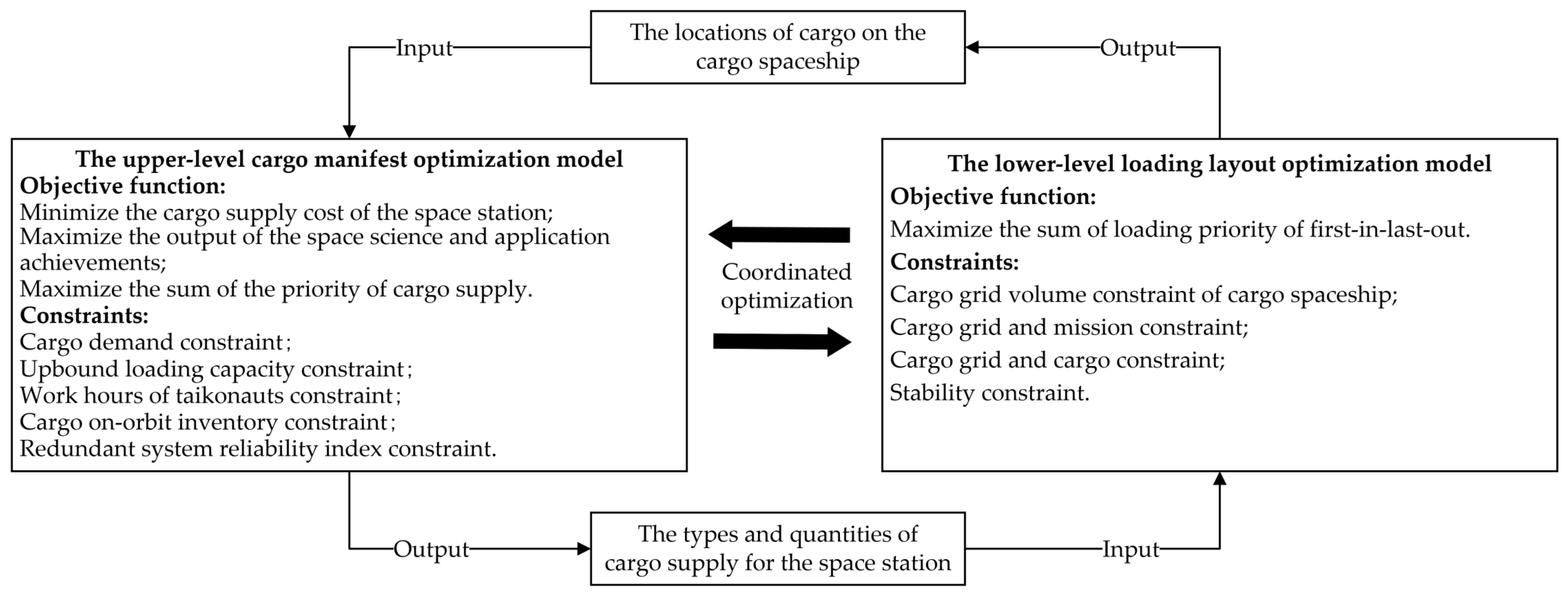
3.6. Framework of Bi-Level Optimization Model
The space station cargo supply planning model is a multi-objective mixed-integer nonlinear programming problem. Equations (2), (9), and (17) are nonlinear. In particular, Constraint (17) is a complex nonlinear, non-convex, and non-differentiable equation that involves variables in product, summation, permutation and combination, and exponentiation operations. This is a complex optimization problem that includes a hierarchical structure. Existing methods struggle to solve this problem directly.
To address this challenge, this study decomposes the space station cargo supply planning model into a bi-level optimization model iterated between the cargo manifest and loading layout. The solution obtained from the upper-level model serves as the input for the lower-level model. The decision made by the lower-level model influences the result of the upper-level model. The framework of the bi-level optimization model is illustrated in Figure 3.
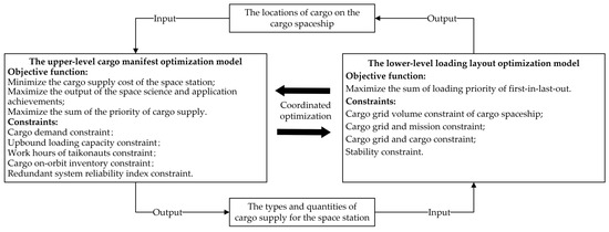
Figure 3.
The framework of the bi-level optimization model.
The upper-level cargo manifest optimization model determines the types and quantities of cargo supplies for the space station without considering the loading layout. The objective functions are (1), (2), and (3). The constraints are (5), (6), (7), (8), (16), (17), (18), (19), (20), and (22). Due to the nonlinearity of objective function (2) and Constraint (17), the upper-level cargo manifest optimization model is a multi-objective mixed-integer nonlinear programming problem.
The lower-level loading layout optimization model determines cargo locations on the cargo spaceship without compromising the optimal objective function value of the upper-level model. The objective function is (4). The constraints are (9), (10), (11), (12), (21), (23), (24), (27), (28), (29), and (30). Since the upper-level cargo manifest optimization model passes the decision variable to the lower-level loading layout optimization model, Constraint (9) becomes linear. Consequently, the lower-level loading layout optimization model is a single-objective 0–1 integer programming problem.
Through the above transformations, this study converts the complex space station cargo supply planning problem into a bi-level optimization problem. A feasible solution approach involves proposing a meta-heuristic method to solve the upper-level cargo manifest optimization model and using an exact method to solve the lower-level loading layout optimization model.
4. Algorithm Design for Space Station Cargo Supply Planning
4.1. Overall Flow of Algorithm
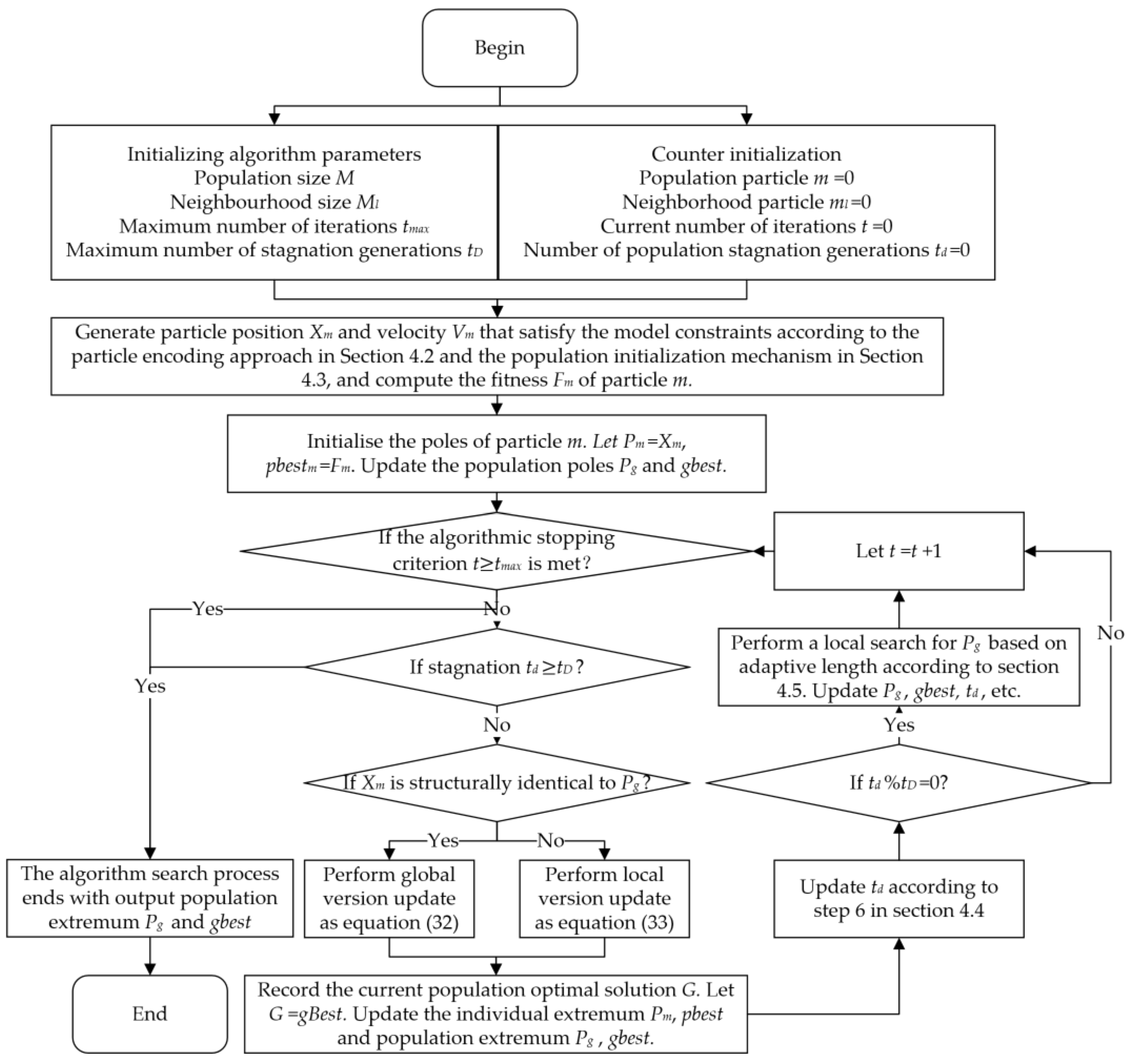
Meta-heuristic algorithms are considered intelligent methods for solving large-scale mixed-integer nonlinear programming problems [34]. Common meta-heuristic algorithms include the genetic algorithm (GA), particle swarm optimization (PSO) algorithm, ant colony optimization (ACO) algorithm, cuckoo search (CS) algorithm, and so on. The upper-level cargo manifest optimization model of the space station cargo supply planning problem can be transformed into a continuous optimization problem. The PSO algorithm has significant advantages in handling such issues. It is more suitable for finding the optimal solution of the cargo manifest optimization model due to its advantages of a memory mechanism [35], fewer parameters [36], and ease of implementation [37]. However, the PSO algorithm has disadvantages such as dependence on initial parameters, premature convergence, and a tendency to fall into local optima [38], making it challenging to find the global optimal solution for the cargo manifest optimization model with multiple peaks. Therefore, it is necessary to further optimize and improve the traditional PSO algorithm. The lower-level loading layout optimization model of the space station cargo supply planning problem can be solved exactly using the branch-and-bound method of CPLEX. The overall flow of the CILPSO algorithm proposed in this study is shown in Figure 4.

Figure 4.
Overall flowchart of the CILPSO algorithm.
4.2. Particle Encoding
For the space station cargo supply planning problem, , , and are the decision variables in the cargo manifest optimization model, and is the decision variable in the loading layout optimization model. Among them, and are considered the primary decision variables, while and are intermediate variables. This study encodes the decision variable . With known, the decision variables and of the cargo manifest optimization model can be solved indirectly through . The decision variable of the loading layout optimization model can be precisely solved using CPLEX.
The particle encoding method is shown in Figure 5. Set the population size as . The position of the particle is , where the -th component denotes the supply quantity of the cargo and takes the value range of . The velocity of the particle m is , and the -th component takes the value range of . The fitness function is represented by the objective function . The local optimal position and fitness of each particle are and , respectively. The global optimal position and fitness of the population are and , respectively.
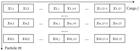
Figure 5.
Particle encoding method.
The quantities of cargo that do not belong to the category of scientific and applied experiments are only related to the total cost of cargo supply in the objective function. Therefore, minimizing the quantity of such cargo is preferable. In this study, we take the minimum value that satisfies the constraints of the cargo list optimization model as the quantity of cargo not belonging to the science and application experiment category. The particle generation in the following section focuses on the supply quantity of the scientific and applied experimental cargo.
4.3. Population Initialization
To optimize the quality of initial solutions and increase their diversity, this study proposes two mechanisms for population initialization: reliability priority and random generation.
Population initialization process:
Step 1: Initialization. The population sizes are and ( 1 or 2, denoting the two initialization mechanisms, respectively). The number of cargo supply types is . Set counters and . Initialize each component of , , and , as well as the fitnesses , , and , to zero.
Step 2: Judge whether ? If yes, execute Step 3; otherwise, execute Step 8.
Step 3: If , execute the cargo reliability priority mechanism; if , execute the random generation mechanism.
Step 4: Judge whether ? If yes, execute Step 5; otherwise, execute Step 7.
Step 5: Can particles be generated according to the initialization mechanism? They must satisfy the Constraints (5), (6), (7), (8), (16), and (17) of the cargo manifest optimization model. Generally, the value range for each non-zero component of is , and the value range for each non-zero component of is . In practice, the algorithm search is accelerated by adjusting the value range for and according to the particular scenario. If particles satisfy the constraints, generate them and execute Step 6; otherwise, gradually reduce the number of cargo types according to the cargo prioritization rule, , and re-execute Step 5.
Step 6: Given the known decision variables , , and , establish the loading layout optimization model. The objective function is Equation (4), and the constraints are Equations (9)–(12), (23), (24) and (27)–(30). Call CPLEX to solve the decision variable . Judge whether a feasible solution exists for the model? If yes, calculate the fitness of particle , and return to Step 4; otherwise, re-execute Step 5.
Step 7: Evaluate the population and initialize the local optimal position and fitness for each particle. Then sort the particles in ascending order based on fitness , and select the top particles as the initial particles of the population. Set , , and return to Step 2.
Step 8: Update the global optimal position and fitness of the population. The population initialization is finished.
The above fitness is the objective function for the cargo manifest optimization model. To facilitate solving, this multi-objective optimization model is transformed into a single-objective one using a weighted sum approach. The linear standardization technique eliminates the different magnitudes among the objective functions. The weights of these objective functions are determined by the AHP method based on expert experience. Among them, , , and denote each objective function after linear standardization, respectively.
4.4. Particle Updating
Considering the different particle structures caused by the different types of upbound cargo, a particle updating method combining global and local versions is proposed.
where denotes the current number of iterations. denotes the maximum number of iterations. denotes the linearly decreasing inertia weight controlling the particle motion. and denote the individual learning factor and the social learning factor. and are random numbers with a value range (0,1). Since the supply quantity of the cargo must be a positive integer, a rounding operation is applied to the successive solutions generated during each iteration after updating the particle positions.
Particle updating process:
Step 1: Initialization. The current number of iterations is . The number of population stagnation generations is . The global optimal fitness of the population, denoted by , equals . Set counter .
Step 2: Judge whether ? If yes, execute Step 3; otherwise, execute Step 6.
Step 3: If the local optimal structure of the particle is consistent with the global optimal structure of the population, execute the global updating method shown in Equation (32); otherwise, execute the local updating method shown in Equation (33).
Step 4: Update the particle positions according to Equation (34) and repair infeasible particles.
Step 5: Evaluate the population. Update the local optimal position and fitness of each particle and the global optimal position and fitness of the population. , return to Step 2.
Step 6: Update the number of population stagnation generations . Judge whether ? If yes, ; otherwise, . The particle updating is finished.
4.5. Local Search Strategy
To address the deficiency of the PSO algorithm’s tendency to fall into local optima, a local search strategy with adaptive neighborhood length is proposed to prevent premature convergence.
The adaptive neighborhood length of the -th component is as follows:
where is used to adaptively adjust the neighborhood length and is set according to the specific problem nature.
Local search strategy:
Step 1: Initialization. The number of population stagnation generations is . The global optimal fitness of the population, denoted by , equals . The random generation neighborhood population size is . For any , , and the adaptive neighborhood length is . Set counters and .
Step 2: Judge whether . If yes, execute Step 3; otherwise, execute Step 6.
Step 3: Judge whether . If yes, execute Step 4; otherwise, execute Step 5.
Step 4: Judge whether is non-zero. If yes, generate randomly in the neighborhood of , , , and return to Step 3; otherwise, , and return to Step 3.
Step 5: Evaluate the particle . Update the local optimal position and fitness of the particle and the global optimal position and fitness of the population. , and return to Step 2.
Step 6: Update the number of population stagnation generations . Judge whether . If yes, ; otherwise, . The local search is finished.
5. Case Study
5.1. Parameter Setting
The case study involves a Tianzhou Cargo Spaceship supplying cargo to the China Space Station. This study focuses on the logical feasibility of space station cargo supply planning. As the China Space Station is in its initial operational stage, the number of launched Tianzhou Cargo Spaceships is limited. This results in a small sample size for cargo supply and an unclear regularity curve. Experimental data are generated through random simulation based on actual data analysis and expert investigation. The rules for generating the parameters of the space station cargo supply planning model are shown in Table 2. Refer to Tables S1 and S2 for the list of experimental parameter values. The case study includes 12,157 constraints, 7801 integer variables, and 5800 binary variables.
Table 2.
Case parameter setup rules.
To validate the effectiveness of the method proposed in this study, we compare the CILPSO algorithm with other algorithms. They are the random search algorithm (RSA), genetic algorithm (GA), differential evolution (DE), an improved PSO algorithm proposed in the literature [39], a CLPSO algorithm with a local search strategy, and a CIPSO algorithm with two types of population initialization mechanisms. The above algorithms are denoted by ALG1-ALG6, respectively.
The algorithms use uniform parameters. The population size is 40. The neighborhood population size is 40. The maximum number of iterations is 100. The maximum number of stagnation generations is 3. The individual learning factor and social learning factor are both 0.5. The maximum velocity inertia factor and the minimum velocity inertia factor are 0.9 and 0.8, respectively. The crossover probability is 0.8. The mutation probability is 0.01. The weights , , and of the objective functions of the cargo manifest optimization model are , , and , respectively.
The hardware environment for the simulation experiments is a Windows 11 system, processor 12th Gen Intel(R) Core(TM) i7-12700H 2.30 GHz, 16 GB of RAM, and a 64-bit operating system. The programming software is MATLAB R2020b, interfacing with IBM ILOG CPLEX 28.2.0 on the GAMS platform.
5.2. Performance Analysis
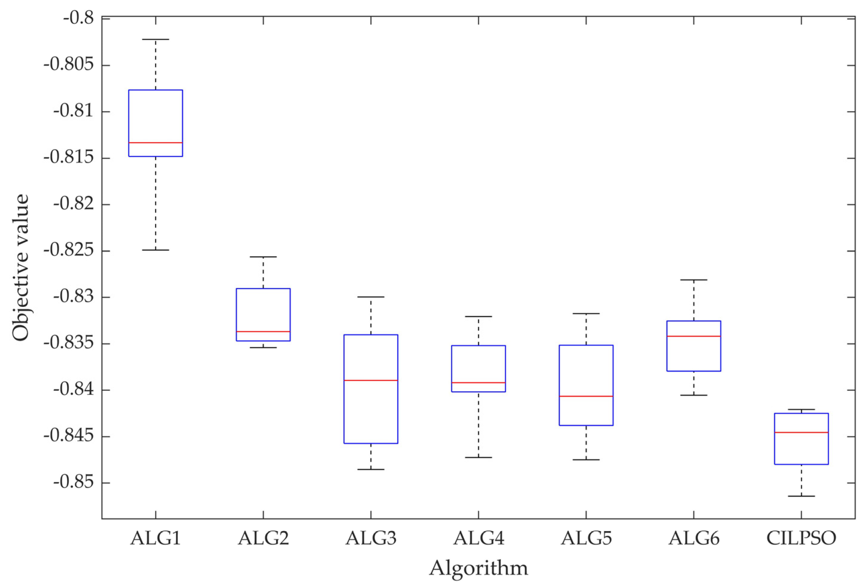
Run the CILPSO algorithm and ALG1-ALG6 each 10 times. The optimal, average, and worst objective values as well as the standard deviation are recorded for each algorithm. The comparison of the search performance among different algorithms is shown in Table 3. As can be seen from Table 3, the optimal objective value , the average objective value , and the worst objective value of the CILPSO algorithm are smaller than those of the other algorithms. This demonstrates that the CILPSO algorithm possesses superior solution quality and the best average search performance.
Table 3.
Comparison of search performances among different algorithms.
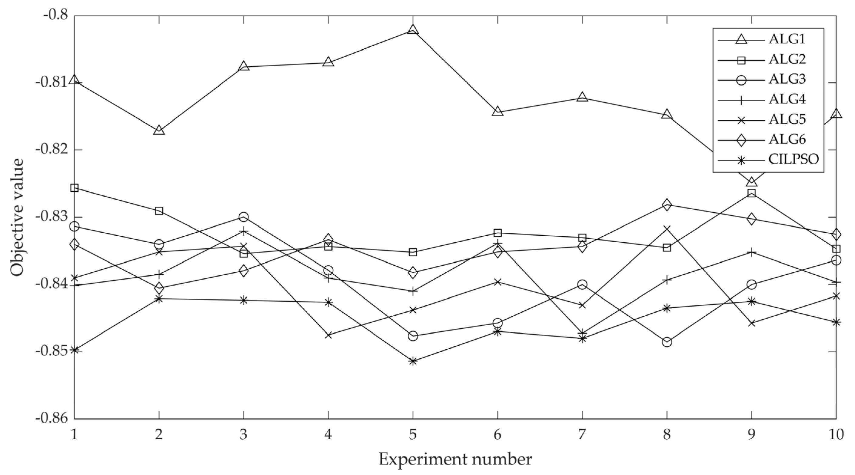
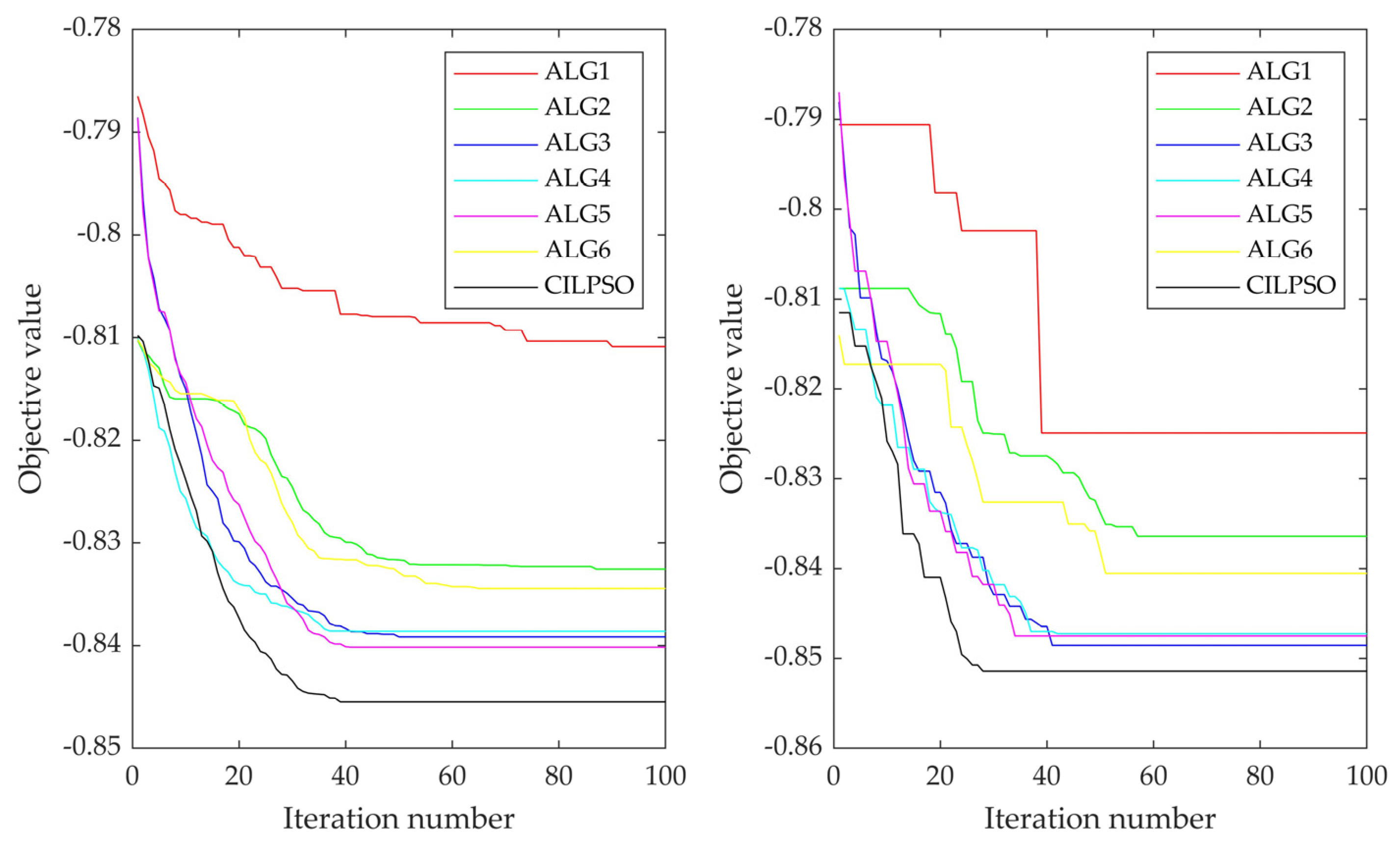
The box plots of the distribution of the objective values are shown in Figure 6. The variation curves of the objective values are shown in Figure 7. According to Table 3, Figure 6 and Figure 7, the standard deviation of the CILPSO algorithm is lower than that of the other algorithms. This suggests that the CILPSO algorithm has stable solutions, good initial value robustness, and superior comprehensive search performance.
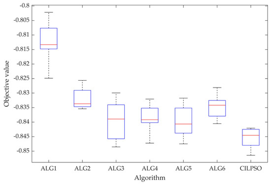
Figure 6.
Box plots of objective value distribution for different algorithms.

Figure 7.
The variation curves of the objective values for different algorithms.
The variation curves of the average objective value and the optimal objective value with evolutionary generations are shown in Figure 8. As shown in Figure 8, the CILPSO algorithm outperforms ALG1-ALG4 in both the average and the optimal objective values with evolutionary generations, proving that the algorithm proposed in this study has a good search performance. Compared with the ALG5 algorithm, the CILPSO algorithm possesses a better initial population and superior search performance, which suggests that the population initialization method proposed in this study is feasible and effective. In the initial stage of algorithm search, both the CILPSO algorithm and the ALG6 algorithm can quickly find better solutions, due to the strong global search capability of the PSO algorithm. However, as the number of iterations increases, the ALG6 algorithm gradually converges. In contrast, the CILPSO algorithm continues to locally search for even better solutions, indicating the feasibility and effectiveness of the local search strategy proposed in this study.
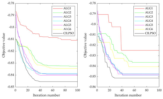
Figure 8.
The variation curves of the average objective value and the optimal objective value with evolutionary generations for different algorithms.
To further verify the optimality performance of the proposed method, this study employs different methods for comparison. A comparison of optimality performance among different algorithms is shown in Table 4. Firstly, the Mann–Whitney U Test is utilized to compare the weighted objective values of CILPSO with ALG1-ALG6 for solving upper-level cargo manifest optimization. The p-values obtained from the Mann–Whitney U Test for ALG1-ALG6 are less than 0.05. Therefore, the null hypothesis is rejected. It can be conclusively stated that CILPSO significantly outperforms ALG1-ALG6 in solving the upper-level cargo manifest optimization problem. Secondly, the relative GAP and solving time of CPLEX are utilized to compare the optimal objective values achieved by different algorithms for the lower-level loading layout optimization. The results show that CPLEX returns solutions with relative GAPs within 10% in less than one second. For the large-scale problem, CPLEX in CILPSO takes 0.38 s to obtain a solution with a relative GAP of 6.14%. This solution is sufficient for practical applications.
Table 4.
Comparison of optimality performance among different algorithms.
To test the convergence performance of the CILPSO algorithm proposed in this study, ALG1 to ALG6 are also compared with the CILPSO algorithm according to the above rules. The average number of convergence generations and average running time are shown in Table 5. As can be seen from the table, compared with ALG1-ALG6, the CILPSO algorithm has a shorter average running time and a smaller average number of convergence generations, which indicates that the CILPSO algorithm has higher search efficiency.
Table 5.
The average number of convergence generations and average running time.
In summary, the CILPSO algorithm can achieve excellent convergence performance while maintaining high search performance. It is suitable for solving the space station cargo supply planning problem that involves large-scale, multi-objective, complex nonlinear, non-convex, non-differentiable, and mixed-integer characteristics.
5.3. Solution Analysis
In practical engineering, without scientific modeling planning, the quantity of cargo on-orbit inventory after cargo spaceship supply is generally maintained at nearly twice the quantity of demand to ensure sufficient reliability of the space station. Compared to this situation, the method proposed in this study reduces the upbound cost of cargo spaceship by 38.40%, saves 37.29% of cargo spaceship space resources, and frees up 36.54% of cargo-handling work hours for taikonauts to carry out space science and application experiments more adequately, while avoiding 37.44% of space orbit waste burning and emission pollution, based on meeting the system reliability of the space station.
Sub-objective function values and weighted objective function values for different algorithms are shown in Table 6. The optimal cargo manifest schemes of different algorithms are shown in Table S3. The optimal loading layout schemes of different algorithms are shown in Tables S4–S10. All algorithms have equal total sums of the priority of cargo supply . This is because the supply status of cargo , represented by , is consistent and always equals 1. This phenomenon indicates that the loading capacity of cargo spaceship and the prescribed maximum total taikonaut work hours handling cargo are sufficient. The total output of the space science and application achievements of the CILPSO algorithm is the largest. This is because the supply quantity of scientific and applied experimental cargo derived by the CILPSO algorithm is generally larger, resulting in a greater weight of the upbound payloads and taikonaut work hours in dealing with scientific and experimental missions. The total cargo supply cost of space station for the CILPSO algorithm is less than those of ALG1-ALG3 and ALG6, but more than those of ALG4 and ALG5. This is mainly due to the larger supply quantity of low-cost scientific and applied experimental cargo of the CILPSO algorithm compared to ALG1-ALG3 and ALG6. Compared to ALG4 and ALG5, the CILPSO algorithm seeks a larger supply quantity of high-cost scientific and applied experimental cargo. The sum of the loading priority of first-in-last-out of the CILPSO algorithm is higher than that of ALG1-ALG4 but lower than those of ALG5-ALG6. This is related to factors such as the supply quantity of cargo, the unit volume of cargo, and the relative GAP of CPLEX.
Table 6.
Sub-objective function values and weighted objective function values for different algorithms.
5.4. Sensitivity Analysis
The decision-making scheme for space station cargo supply planning is closely related to the values of model parameters. This section mainly analyzes the impact of changes in the objective function weights, loading capacity, maximum total work hours, and cargo grid volume on the cargo manifest scheme and the loading layout scheme.
Firstly, this study explores the impact of changes in the objective function weights. Since balancing the cargo supply cost and the output of space science and application achievements is the focus of this study, the objective function weight of the cargo priority is fixed at 0.4. The analysis then focuses on how the cargo manifest scheme and the loading layout scheme vary with changes in the objective function weights of cargo supply cost and the output of the space science and application achievements.
The impact of changes in the objective function weights on the optimal objective value of the cargo manifest optimization is shown in Figure 9. Optimal cargo manifest schemes for different objective function weight combinations are shown in Table S11. It can be seen that when the value of gradually decreases, the optimal objective value of the cargo manifest optimization decreases in an approximately linear manner. The changes in the objective function weights do not impact the quantity of cargo supply for taikonaut health missions and platform safety operation missions. However, the quantity of cargo supply for scientific and applied experimental missions is more sensitive to the objective function weights. When the decision-maker prefers reducing the cargo supply cost of the space station, i.e., , the quantity of cargo supply for scientific and applied experimental missions is lower. Conversely, when the decision-maker prefers increasing the output of space science and application achievements, i.e., , the quantity of cargo supply for scientific and applied experimental missions is higher. This is because the changes in the objective function weights are equivalent to changing the parameter coefficient values of unit cost, the product of unit weight, and unit work hours of cargo for scientific and applied experimental missions.
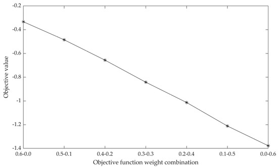
Figure 9.
The impact of changes in the objective function weights on the optimal objective value of the cargo manifest optimization.
The optimal objective values for the loading layout optimization under different objective function weight combinations are shown in Table 7. Optimal loading layout schemes are shown in Tables S12–S18. As shown in the table, there is no obvious change in the loading layout scheme under different objective function weight combinations. This is mainly related to the sufficient cargo grid volume not affecting the loading layout of cargo within the cargo spaceship.
Table 7.
Optimal objective values for the loading layout optimization under different objective function weight combinations.
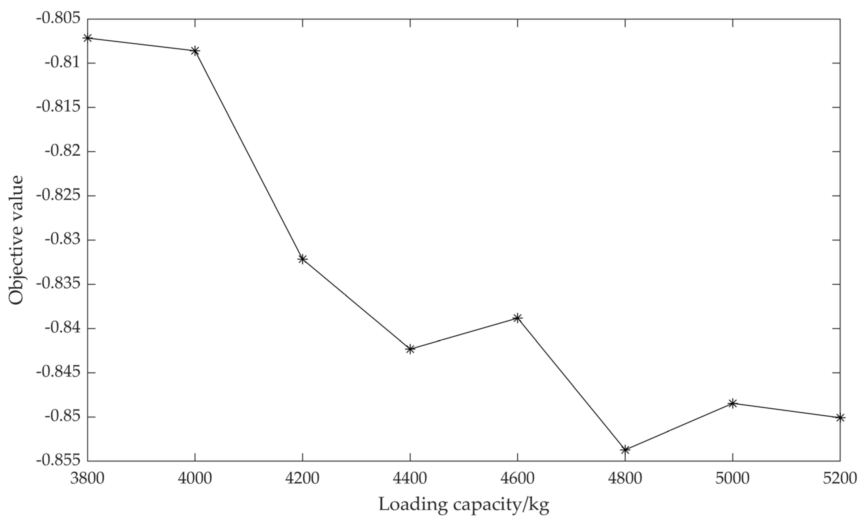
Secondly, the impact of loading capacity changes is discussed. The impact of changes in loading capacity on the optimal objective value for the cargo manifest optimization is shown in Figure 10. Optimal cargo manifest schemes for different loading capacities are shown in Table S19. When the loading capacity falls below 4400 kg, owing to insufficient loading capacity to support part of the cargo to ascend and reduced quantities for the scientific and applied experimental missions, the optimal objective value of the cargo manifest optimization increases as the loading capacity decreases. Decisions of whether to supply cargo and the quantity of cargo supply are susceptible to fluctuations in loading capacity. However, once the loading capacity exceeds 4400 kg, the optimal objective value for the cargo manifest optimization fluctuates due to a trade-off between the cost of cargo supply and the output of the achievements for scientific and applied experimental missions.

Figure 10.
The impact of changes in loading capacity on the optimal objective value of the cargo manifest optimization.
The optimal objective values for the loading layout optimization under different loading capacities are shown in Table 8. Optimal loading layout schemes are shown in Tables S20–S27. When the loading capacity does not exceed 4400 kg, for the same reason mentioned above, the missions occupy less space and are loaded closer to the exit hatch of the cargo spaceship. Consequently, the optimal objective value of the loading layout optimization increases as the loading capacity decreases. When the loading capacity exceeds 4400 kg, the change in the loading layout scheme is not obvious due to the sufficient loading capacity.
Table 8.
The optimal objective values for the loading layout optimization under different loading capacities.
To summarize, in the research on space station cargo supply planning, the first step is to determine the objective preference of the decision-maker. The quantity of cargo supply for scientific and applied experimental missions is susceptible to changes in the objective function weights. Secondly, both the cargo manifest scheme and the loading layout scheme are sensitive to variations in loading capacity. Therefore, reasonable loading capacity should be designed to meet the cargo supply demands of the space station while avoiding space waste. Moreover, the maximum total work hours and cargo grid volume, both with properties similar to loading capacity, should be considered accordingly.
6. Conclusions
With the China Space Station fully operational, integrating information from various systems has become critical. This integration enables scientific and reasonable cargo supply planning, ultimately enhancing the efficiency of space resource utilization. However, this problem exhibits numerous challenging characteristics, including large-scale, multi-objective, complex nonlinear, non-convex, non-differentiable, and mixed-integer attributes. These characteristics render existing solution methods inapplicable. In this study, the problem is decomposed into a bi-level optimization problem that iterates between the cargo manifest and the loading layout. Additionally, a new CILPSO algorithm is proposed, which integrates particle coding, reliability priority, and random generation mechanisms of population initialization, global and local versions of particle updating, and a local search strategy. Experimental results demonstrate that the proposed cargo supply planning method optimizes at least 35% of various space resources, including cargo upbound cost, spaceship occupancy volume, taikonaut work hours, and space waste burned and discharged in orbit. Moreover, the CILPSO algorithm exhibits superior search and convergence performance compared to other algorithms. Therefore, the result could be considered a reference for developing cargo supply schemes, submitting cargo demands, and designing loading schemes. It can reduce cargo supply costs, enhance space science and application outputs, and promote the transformation of space station logistics toward a sustainable and eco-friendly model. Beyond the space station, the proposed method can be applied to other planning problems with similar characteristics. Future research will focus on the standardization, normalization, and modeling of supply cargo for a mature space station. Additionally, the uncertainty of demand for non-spare and spare parts can be expressed through interval numbers and scenario modeling, establishing a two-level stochastic mixed-integer nonlinear cargo supply planning model. This may result in planning outcomes that are more aligned with real-world scenarios.
Supplementary Materials
The following supporting information can be downloaded at https://www.mdpi.com/article/10.3390/su16156488/s1, Table S1: List of experimental parameter values; Table S2: Experimental parameter values of ; Table S3: Optimal cargo manifest schemes of different algorithms; Table S4: Optimal loading layout scheme of ALG1; Table S5: Optimal loading layout scheme of ALG2; Table S6: Optimal loading layout scheme of ALG3; Table S7: Optimal loading layout scheme of ALG4; Table S8: Optimal loading layout scheme of ALG5; Table S9: Optimal loading layout scheme of ALG6; Table S10: Optimal loading layout scheme of CILPSO; Table S11: Optimal cargo manifest schemes for different objective function weight combinations; Table S12: Optimal loading layout scheme for –(0.6–0.0); Table S13: Optimal loading layout scheme for (0.5–0.1); Table S14: Optimal loading layout scheme for (0.4–0.2); Table S15: Optimal loading layout scheme for (0.3–0.3); Table S16: Optimal loading layout scheme for (0.2–0.4); Table S17: Optimal loading layout scheme for (0.1–0.5); Table S18: Optimal loading layout scheme for (0.0–0.6); Table S19: Optimal cargo manifest schemes for different loading capacities; Table S20: Optimal loading layout scheme for (3800); Table S21: Optimal loading layout scheme for (4000); Table S22: Optimal loading layout scheme for (4200); Table S23: Optimal loading layout scheme for (4400); Table S24: Optimal loading layout scheme for (4600); Table S25: Optimal loading layout scheme for (4800); Table S26: Optimal loading layout scheme for (5000); Table S27: Optimal loading layout scheme for (5200).
Author Contributions
Conceptualization, Z.K., M.G. and W.D.; methodology, Z.K.; software, Z.K.; validation, Z.K., M.G., W.D. and J.W.; formal analysis, Z.K., M.G. and W.D.; investigation, Z.K., M.G., W.D. and J.W.; resources, Z.K. and W.D.; data curation, Z.K.; writing—original draft preparation, Z.K.; writing—review and editing, Z.K., M.G., W.D. and J.W.; visualization, Z.K.; supervision, W.D.; project administration, Z.K.; funding acquisition, W.D. All authors have read and agreed to the published version of the manuscript.
Funding
This research was funded by the Overall Special Project of Space Application System in the Application and Development Stage of China Space Station Engineering (T014191).
Institutional Review Board Statement
Not applicable.
Informed Consent Statement
Not applicable.
Data Availability Statement
Data are contained within the article and Supplementary Materials.
Acknowledgments
Special thanks to the team led by Luhua Xi of the Operation and Management Support Center of China Manned Space Program for supporting the cargo management business for the China Space Station.
Conflicts of Interest
The authors declare no conflicts of interest.
Appendix A
The detailed derivation process of Constraint (17) is as follows.
(1) System reliability model theory.
Reliability refers to the probability that a product does not break down during use.
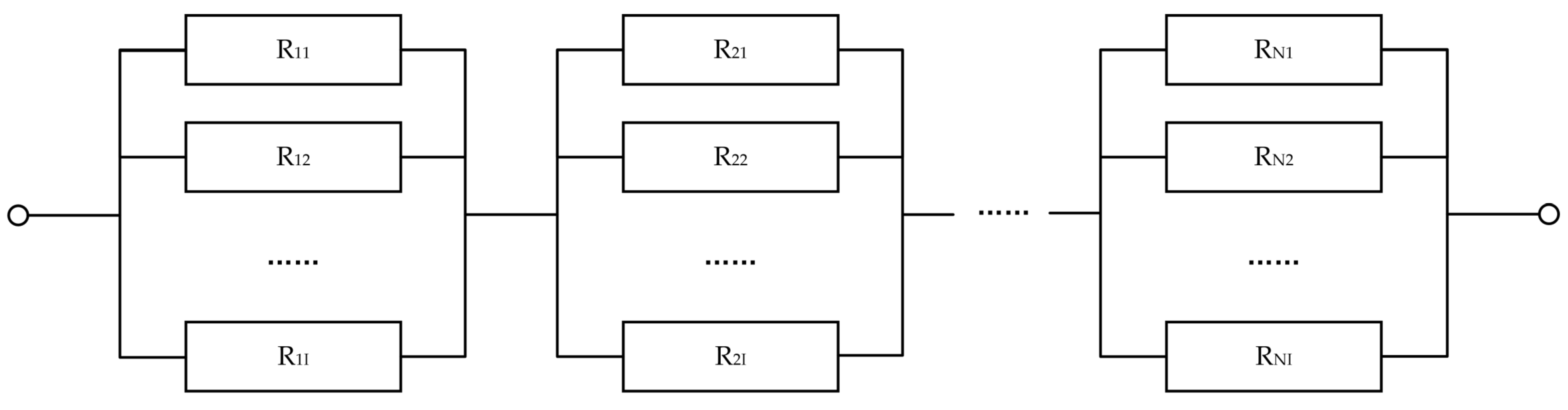
(a) Reliability of series-parallel system.
For the series-parallel system of Figure A1, the reliability is as follows:
represents the reliability of the series-parallel system.
represents the number of series connections.
represents the number of parallel connections.
represents the product reliability of the -th parallel connection in the -th series connection.

Figure A1.
Series-parallel system.
Figure A1.
Series-parallel system.
(b) Reliability of redundant system.
For the redundant system with a redundancy level , there are subsystems. As long as at least subsystems can work normally, the system can work normally. Assuming that the voter is completely reliable, the reliability of each subsystem is . The reliability of the redundant system is as follows:
(2) Redundancy system reliability model of space station cargo supply.
The redundancy system of the space station cargo supply is shown in Figure A2. The redundancy level of each cargo for each mission is .
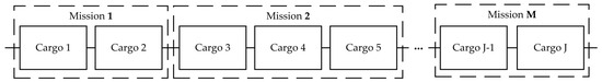
Figure A2.
Redundancy system of the space station cargo supply.
Figure A2.
Redundancy system of the space station cargo supply.
Based on the system reliability model theory, the reliability constraint of each mission is given by Constraint (17).
References
- Gao, M.; Zhao, G.H.; Gu, Y.D. Space science and application mission in China’s space station. Bull. Chin. Acad. Sci. 2015, 30, 721–732. [Google Scholar]
- Lin, K.P.; Luo, Y.Z.; Tang, G.J. Optimization of Logistics Strategies for Long-Duration Space-Station Operation. J. Spacecr. Rocket. 2014, 51, 1709–1720. [Google Scholar] [CrossRef]
- Lin, K.P.; Luo, Y.Z.; Tang, G.J. Multi-objective optimization of space station logistics strategies using physical programming. Eng. Optimiz. 2015, 47, 1140–1155. [Google Scholar] [CrossRef]
- Zhu, Y.H.; Luo, Y.Z. Multi-objective optimisation and decision-making of space station logistics strategies. Int. J. Syst. Sci. 2016, 47, 3132–3148. [Google Scholar] [CrossRef]
- Gralla, E.; Shull, S.; de Weck, O. A modeling framework for interplanetary supply chains. In Proceedings of the Space 2006, San Jose, CA, USA, 19–21 September 2006; Available online: https://arc.aiaa.org/doi/abs/10.2514/6.2006-7229 (accessed on 25 May 2024).
- Taylor, C.; Song, M.; Klabjan, D.; de Weck, O.; Simchi-Levi, D. Modeling interplanetary logistics: A mathematical model for mission planning. In Proceedings of the SpaceOps 2006 Conference, Rome, Italy, 19–23 June 2006; Available online: https://arc.aiaa.org/doi/pdf/10.2514/6.2006-5735 (accessed on 25 May 2024).
- Taylor, M.C.; de Weck, P.O.; Klabjan, P.D. Integrated Transportation System Design for Space Exploration Logistics. In Proceedings of the 57th International Astronautical Congress, Valencia, Spain, 2–6 October 2006; Available online: https://arc.aiaa.org/doi/abs/10.2514/6.IAC-06-D1.3.08 (accessed on 25 May 2024).
- Siddiqi, A.; Shull, S.; de Weck, O. Matrix Methods Analysis of International Space Station Logistics. In Proceedings of the AIAA SPACE 2008 Conference & Exposition, San Diego, CA, USA, 9–11 September 2008; Available online: https://arc.aiaa.org/doi/abs/10.2514/6.2008-7605 (accessed on 25 May 2024).
- Siddiqi, A.; de Weck, O.L.; Lee, G.Y.; Shull, S.A. Matrix Modeling Methods for Spaceflight Campaign Logistics Analysis. J. Spacecr. Rocket. 2009, 46, 1037–1048. [Google Scholar] [CrossRef]
- Grogan, P.T.; Siddiqi, A.; de Weck, O.L. Matrix Methods for Optimal Manifesting of Multinode Space Exploration Systems. J. Spacecr. Rocket. 2011, 48, 679–690. [Google Scholar] [CrossRef]
- Grogan, P.; Yue, H.; De Weck, O. Space logistics modeling and simulation analysis using spacenet: Four application cases. In Proceedings of the AIAA Space 2011 Conference & Exposition, Long Beach, CA, USA, 27–29 September 2011; Available online: https://arc.aiaa.org/doi/abs/10.2514/6.2011-7346 (accessed on 25 May 2024).
- Ho, K.; Green, J.; De Weck, O. Integrated framework for the design of crewed space habitats and their supporting logistics system. In Proceedings of the AIAA SPACE 2012 Conference & Exposition, Pasadena, CA, USA, 11–13 September 2012; Available online: https://arc.aiaa.org/doi/abs/10.2514/6.2012-5321 (accessed on 25 May 2024).
- Ho, K.; Green, J.; de Weck, O. Concurrent Design of Scientific Crewed Space Habitats and Their Supporting Logistics System. J. Spacecr. Rocket. 2014, 51, 76–85. [Google Scholar] [CrossRef]
- Ho, K.; Green, J.; De Weck, O. Improved concurrent optimization formulation of crewed space habitats and their supporting logistics systems. In Proceedings of the AIAA Space 2013 Conference and Exposition, San Diego, CA, USA, 10–12 September 2013; Available online: https://arc.aiaa.org/doi/abs/10.2514/6.2013-5413 (accessed on 25 May 2024).
- Lim, Y.F.; Jiu, S.; Ang, M. Integrating Anticipative Replenishment Allocation with Reactive Fulfillment for Online Retailing Using Robust Optimization. Manuf. Serv. Oper. Manag. 2021, 23, 1616–1633. [Google Scholar] [CrossRef]
- Fathi, M.; Ghobakhloo, M. Enabling Mass Customization and Manufacturing Sustainability in Industry 4.0 Context: A Novel Heuristic Algorithm for in-Plant Material Supply Optimization. Sustainability 2020, 12, 6669. [Google Scholar] [CrossRef]
- Wang, H.; Tao, J.Q.; Peng, T.; Brintrup, A.; Kosasih, E.E.; Lu, Y.Q.; Tang, R.Z.; Hu, L.K. Dynamic inventory replenishment strategy for aerospace manufacturing supply chain: Combining reinforcement learning and multi-agent simulation. Int. J. Prod. Res. 2022, 60, 4117–4136. [Google Scholar] [CrossRef]
- Rosales, C.R.; Magazine, M.J.; Rao, U.S. Dual Sourcing and Joint Replenishment of Hospital Supplies. IEEE Trans. Eng. Manag. 2020, 67, 918–931. [Google Scholar] [CrossRef]
- Vanbrabant, L.; Verdonck, L.; Mertens, S.; Caris, A. Improving hospital material supply chain performance by integrating decision problems: A literature review and future research directions. Comput. Ind. Eng. 2023, 180, 31. [Google Scholar] [CrossRef]
- Joia-Sanchez, A.F.; Serpa, J.C. Inventory in Times of War. Manag. Sci. 2021, 67, 6457–6479. [Google Scholar] [CrossRef]
- Zhang, L. Emergency supplies reserve allocation within government-private cooperation: A study from capacity and response perspectives. Comput. Ind. Eng. 2021, 154, 10. [Google Scholar] [CrossRef]
- Shi, Y.; Yang, J.; Han, Q.; Song, H.; Guo, H. Optimal decision-making of post-disaster emergency material scheduling based on helicopter–truck–drone collaboration. Omega 2024, 127, 103104. [Google Scholar] [CrossRef]
- Christensen, F.M.M.; Jonsson, P.; Dukovska-Popovska, I.; Steger-Jensen, K. Information sharing for replenishment planning and control in fresh food supply chains: A planning environment perspective. Prod. Plan. Control. 2023, 34, 1371–1392. [Google Scholar] [CrossRef]
- Bilican, M.S.; Iris, Ç.; Karatas, M. A collaborative decision support framework for sustainable cargo composition in container shipping services. Ann. Oper. Res. 2024, 1–33. [Google Scholar] [CrossRef]
- Brandt, F.; Nickel, S. The air cargo load planning problem—A consolidated problem definition and literature review on related problems. Eur. J. Oper. Res. 2019, 275, 399–410. [Google Scholar] [CrossRef]
- Seixas, M.P.; Mendes, A.B.; Pereira Barretto, M.R.; da Cunha, C.B.; Brinati, M.A.; Cruz, R.E.; Wu, Y.; Wilson, P.A. A heuristic approach to stowing general cargo into platform supply vessels. J. Oper. Res. Soc. 2016, 67, 148–158. [Google Scholar] [CrossRef]
- Vancroonenburg, W.; Verstichel, J.; Tavernier, K.; Vanden Berghe, G. Automatic air cargo selection and weight balancing: A mixed integer programming approach. Transp. Res. Part E Logist. Transp. Rev. 2014, 65, 70–83. [Google Scholar] [CrossRef]
- Iris, Ç.; Christensen, J.; Pacino, D.; Ropke, S. Flexible ship loading problem with transfer vehicle assignment and scheduling. Transp. Res. Part B Methodol. 2018, 111, 113–134. [Google Scholar] [CrossRef]
- Zhou, G.; Li, D.; Bian, J.; Zhang, Y. Airfreight forwarder’s shipment planning: Shipment consolidation and containerization. Comput. Oper. Res. 2024, 161, 106443. [Google Scholar] [CrossRef]
- Jaber, A.; Lafon, P.; Younes, R. A branch-and-bound algorithm based on NSGAII for multi-objective mixed integer nonlinear optimization problems. Eng. Optimiz. 2022, 54, 1004–1022. [Google Scholar] [CrossRef]
- Artis, R.; Shivaie, M.; Weinsier, P.D. A flexibility-based multi-objective model for contingency-constrained transmission expansion planning incorporating large-scale hydrogen/compressed-air energy storage systems and wind/solar farms. J. Energy Storage 2023, 70, 18. [Google Scholar] [CrossRef]
- Chen, Y.F.; Joo, Y.H.; Song, D.R. Multi-Objective Optimisation for Large-Scale Offshore Wind Farm Based on Decoupled Groups Operation. Energies 2022, 15, 2336. [Google Scholar] [CrossRef]
- Patrick, D.T.; Andre, K. Practical Reliability Engineering, 5th ed.; John Wiley & Sons: Hoboken, NJ, USA, 2011; pp. 134–176. ISBN 978-04-7097-982-2. [Google Scholar]
- Farmand, N.; Zarei, H.; Rasti-Barzoki, M. Two meta-heuristic algorithms for optimizing a multi-objective supply chain scheduling problem in an identical parallel machines environment. Int. J. Ind. Eng. Comput. 2021, 12, 249–272. [Google Scholar] [CrossRef]
- Chaitanya, K.; Somayajulu, D.; Krishna, P.R. Memory-based approaches for eliminating premature convergence in particle swarm optimization. Appl. Intell. 2021, 51, 4575–4608. [Google Scholar] [CrossRef]
- Ren, M.L.; Huang, X.D.; Zhu, X.X.; Shao, L.J. Optimized PSO algorithm based on the simplicial algorithm of fixed point theory. Appl. Intell. 2020, 50, 2009–2024. [Google Scholar] [CrossRef]
- Dereli, S.; Köker, R. Strengthening the PSO algorithm with a new technique inspired by the golf game and solving the complex engineering problem. Complex Intell. Syst. 2021, 7, 1515–1526. [Google Scholar] [CrossRef]
- Houssein, E.H.; Gad, A.G.; Hussain, K.; Suganthan, P.N. Major Advances in Particle Swarm Optimization: Theory, Analysis, and Application. Swarm Evol. Comput. 2021, 63, 39. [Google Scholar] [CrossRef]
- Nasrollah, S.; Najafi, S.E.; Bagherzadeh, H.; Rostamy-Malkhalifeh, M. An enhanced PSO algorithm to configure a responsive-resilient supply chain network considering environmental issues: A case study of the oxygen concentrator device. Neural Comput. Appl. 2023, 35, 2647–2678. [Google Scholar] [CrossRef] [PubMed]


Disclaimer/Publisher’s Note: The statements, opinions and data contained in all publications are solely those of the individual author(s) and contributor(s) and not of MDPI and/or the editor(s). MDPI and/or the editor(s) disclaim responsibility for any injury to people or property resulting from any ideas, methods, instructions or products referred to in the content. |
© 2024 by the authors. Licensee MDPI, Basel, Switzerland. This article is an open access article distributed under the terms and conditions of the Creative Commons Attribution (CC BY) license (https://creativecommons.org/licenses/by/4.0/).