The Influence of Structural Parameters on the Ultimate Strength Capacity of a Designed Vertical Axis Turbine Blade for Ocean Current Power Generators

Abstract

An ocean current power generator is a power plant that uses kinetic energy from ocean currents to generate electricity. Considering that the blade is the component that receives the biggest load from seawater currents, its structural design should be strong enough to sustain the applied load. Therefore, this research seeks a suitable design and material for turbine blades using the finite element method (FEM). A NACA 0021 blade with a total length of 3600 mm is used for the base geometry. A parametric study was conducted by varying the spacing between the supports, the pitch angle, the material, and the frame model. Considering a high load, the suitable amount of space between the stiffeners was 2200 mm. It was found that a pitch angle variation between −20° and +20° did not significantly affect the strength of the blade structure. The frame geometry variation caused the rigidity and cross-section area of the blade to differ. Therefore, web-shaped or bar-shaped frames are preferable because they have optimal maximum load-to-weight ratios. The material variation analysis resulted in CFRP material being chosen because it had a high maximum load/weight ratio and a high maximum stress.

1. Introduction

With up to 71% of the Earth’s surface covered by oceans, the ocean is the most prevalent element on the planet [1]. It also offers renewable energy potential through the harnessing of seawater heat [2] and kinetic energy [3,4]. A prime example of how to utilize kinetic energy is through ocean current power plants [3,5], which primarily comprise turbines and generators. In these plants, the turbines convert the translational velocity of ocean currents into rotational velocity, which is then transmitted to the generator [6]. The generator, equipped with magnets and windings, converts this rotational speed into electrical energy [7].

There are two main types of turbines used in ocean current power plants, according to the orientation of the rotating axis. The first type is the horizontal-axis ocean current turbine [8,9], which utilizes a horizontally rotating axis and is typically mounted on a fixed platform [10]. An example of this can be seen in Figure 1a. The second type is the vertical-axis ocean current turbine [11], which features a vertically rotating axis and is more commonly found on floating platforms [12,13]. This setup is depicted in Figure 1b.

This research primarily focuses on the vertical-axis ocean current turbine, chosen for its flexibility and mobility due to its typical attachment to floating platforms [16]. Numerous studies have explored this technology. Nguyen et al. investigated the impact of the blade pitch angle on hydrodynamics [17]. Similarly, Hasankhani et al. examined the hydrodynamics of vertical-axis ocean current turbines under various environmental conditions, including during hurricanes [18]. In 2020, Chen et al. conducted research on blade design for these turbines at low speeds to enhance energy collection efficiency [19]. Huang-Ming et al. performed numerical analyses to assess the energy-converging efficiency of ducts in vertical-axis tidal current turbines in constrained waters [20]. Furthermore, Satrio et al. explored the potential of introducing flow disturbances to improve the hydrodynamic performance of these turbines [21]. From these studies, there has been much research on the hydrodynamics of vertical-axis ocean current generators [22]. However, there has still been no research that investigates the structural strength of this type of power plant. Therefore, this study investigates the construction of the vertical-axis ocean current generator.

Since the turbine blade is directly exposed to ocean currents, it is one of the most heavily loaded components in an ocean current power generator [23]. Consequently, it is crucial that the turbine blade is designed to withstand the applied loads. In light of this, this study investigates the structural integrity of the turbine blade, considering various factors that could affect its ultimate strength. These factors include the spacing between the supporting frames, the selection of materials, the design of the frames, and the pitch angle of the blades.

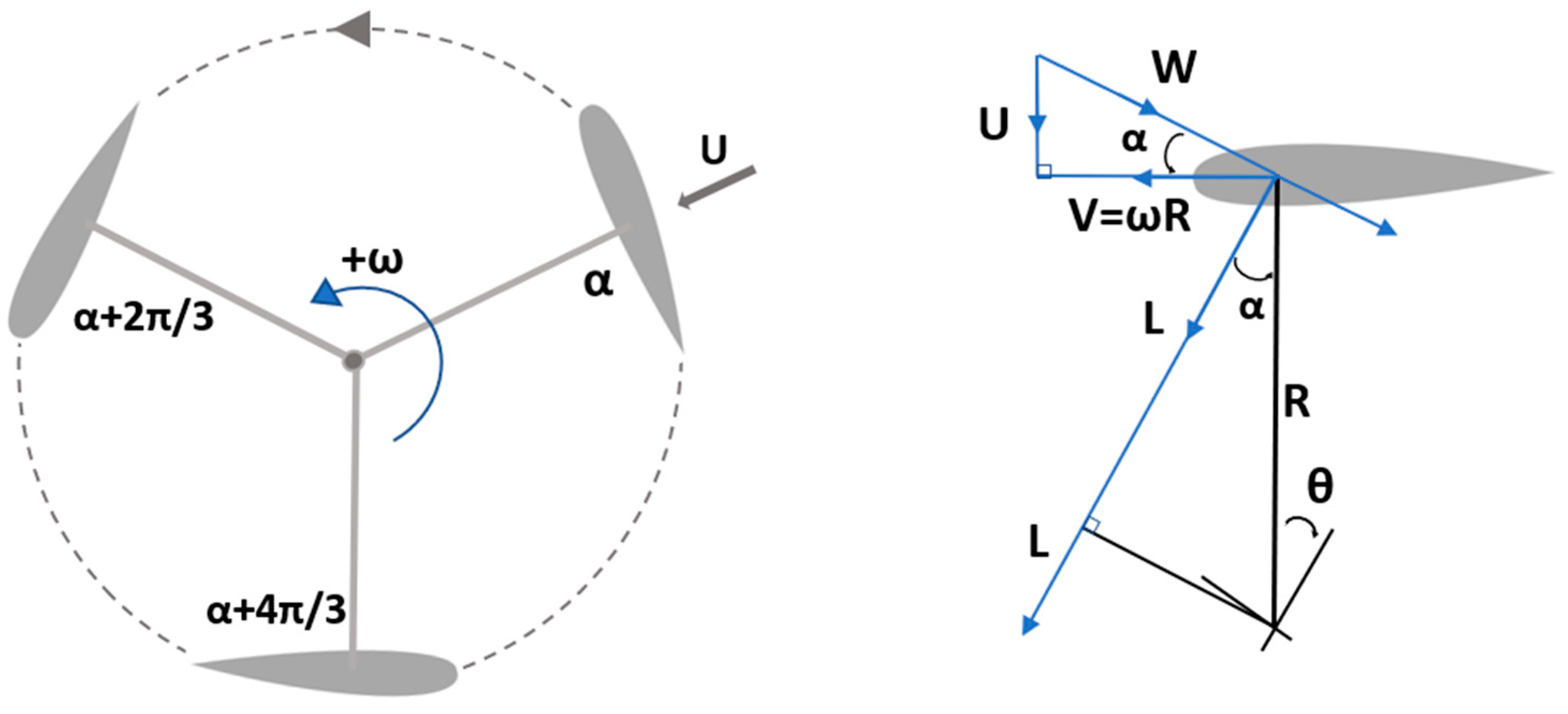
2. Turbine Configuration

A foil, commonly known as the fluid dynamics profile, is a cross-sectional shape designed to generate lift when subjected to fluid flow, whether in air or liquid. This profile is primarily used in devices like propellers and turbine blades [24]. An illustration of this profile can be seen in Figure 2.

The Darrieus hydrokinetics turbine is a turbine with a rotating axis in the vertical direction. This type of turbine has a greater power generation capacity than other types of hydrokinetics turbines in the same area [26]. The easy and inexpensive design and manufacturing of this type of turbine is its main advantage.

In 2023, Asadbeigi et al. conducted a numerical study on a specific type of turbine. Their research focused on various factors, including the number of blades, the profile of the blade foil, and the sphericity of the blades. Their findings indicated that the optimal number of blades for a H-Darrieus turbine is three. Moreover, the blade foil profile that yielded the highest power coefficient was identified as NACA0021 [27]. Consequently, this study employed a H-Darrieus configuration with three blades and used the NACA0021 foil profile. An illustration of the blade configuration can be found in Figure 3.

The Darrieus turbine operates by generating lift and drag forces on a hydrofoil blade within a water flow. The combined tangential force resulting from the lift and drag causes the turbine to rotate. The angle of attack (α) is the angle between the blade’s pitch position and the flow of ocean currents, which move in a singular direction [28]. This can occur because the turbine continues to rotate, causing an angle between the blade and the current flow [29]. An illustration depicting the angle of attack and the generation of lift and drag forces is provided Figure 4. As illustrated in Figure 4, the angle of attack, in combination with the pitch angle, influences the direction of the loading condition set in the analysis. Therefore, structural blade response will also be investigated in this study by imposing forced displacement in two loading directions.

3. Finite Element Method

The finite element method (FEM) is a numerical technique that involves modeling a structure and dividing it into smaller elements, known as a mesh [30]. After meshing, interactions are made on the elements at certain points (nodes). Subsequent calculations are performed at each node using predetermined mathematical formulas. An example of meshing can be seen in Figure 5.

The FEM involves three principal stages: setup, calculation, and result analysis. During setup, the process includes modeling the geometry, defining materials, creating a mesh, and setting boundary conditions [31]. In the calculation stage, numerical calculations are executed at each node defined during setup. After completing these calculations, the results must be analyzed to draw conclusions and interpret the data effectively [32].

Non-linear analysis is an analysis that uses iteration, and large deflections can be used. Iteration is used so that the results of the calculations performed have converged. Basic formula for statics analysis in finite element methods can be seen in Equation (1).

$$\left\{F\right\}=\left[K\right]\left\{u\right\}$$

(1)

The convergence formula applied in the finite element method is shown in Equation (2).

$$F^N\left(u^M\right)=0$$

(2)

In this context, $F^N$ represents the force component, $u^M$ denotes the nodal displacement component, and $K$ stands for the stiffness matrix. The equation is a convergence equation, where when the applied force is added it does not cause deflection, indicating that the calculation has converged [33]. The calculations performed in a finite element method use the Newton–Rahpson method [34]. This method uses linear approximation and achieves convergence faster than other methods. For the 1-dimensional case, it is necessary to know the solution of the equation $g\left(x\right)=0$, where $g:D(D\subset \mathbb{R})\to \mathbb{R}$, also assuming that the function g has first and second derivatives defined in the domain. Then, the Newton–Raphson equation can be written on the function of $g\left(x\right)$ in Equation (3) [35]. In finite element methods, the $g\left(x\right)$ can be substituted with $\left\{F\right\}$.

$$x_{n+1}=x_n-{\displaystyle \frac{g\left(x_n\right)}{g^{\prime }\left(x_n\right)}}$$

(3)

The critical point of a structure is determined by determining the von Mises stress, which combines various stress components on a stress plane. A structure will begin to yield when the von Mises stress exceeds the material’s yield stress (${\sigma }_v>{\sigma }_Y$). The von Mises stress formula is presented in Equation (4) [36].

$${\sigma }_v=\sqrt{{\displaystyle \frac{{{(\sigma }_{xx}-{\sigma }_{yy})}^2+{{(\sigma }_{yy}-{\sigma }_{zz})}^2+{{(\sigma }_{zz}-{\sigma }_{xx})}^2+6{{(\sigma }_{xy}}^2+{{\sigma }_{yz}}^2+{{\sigma }_{zx}}^2)}{2}}}$$

(4)

where ${\sigma }_v$ is the von Mises stress, ${\sigma }_{xx}$ is the x stress component, ${\sigma }_{yy}$ is the y stress component, and ${\sigma }_{zz}$ is the z stress component.

4. Methodology

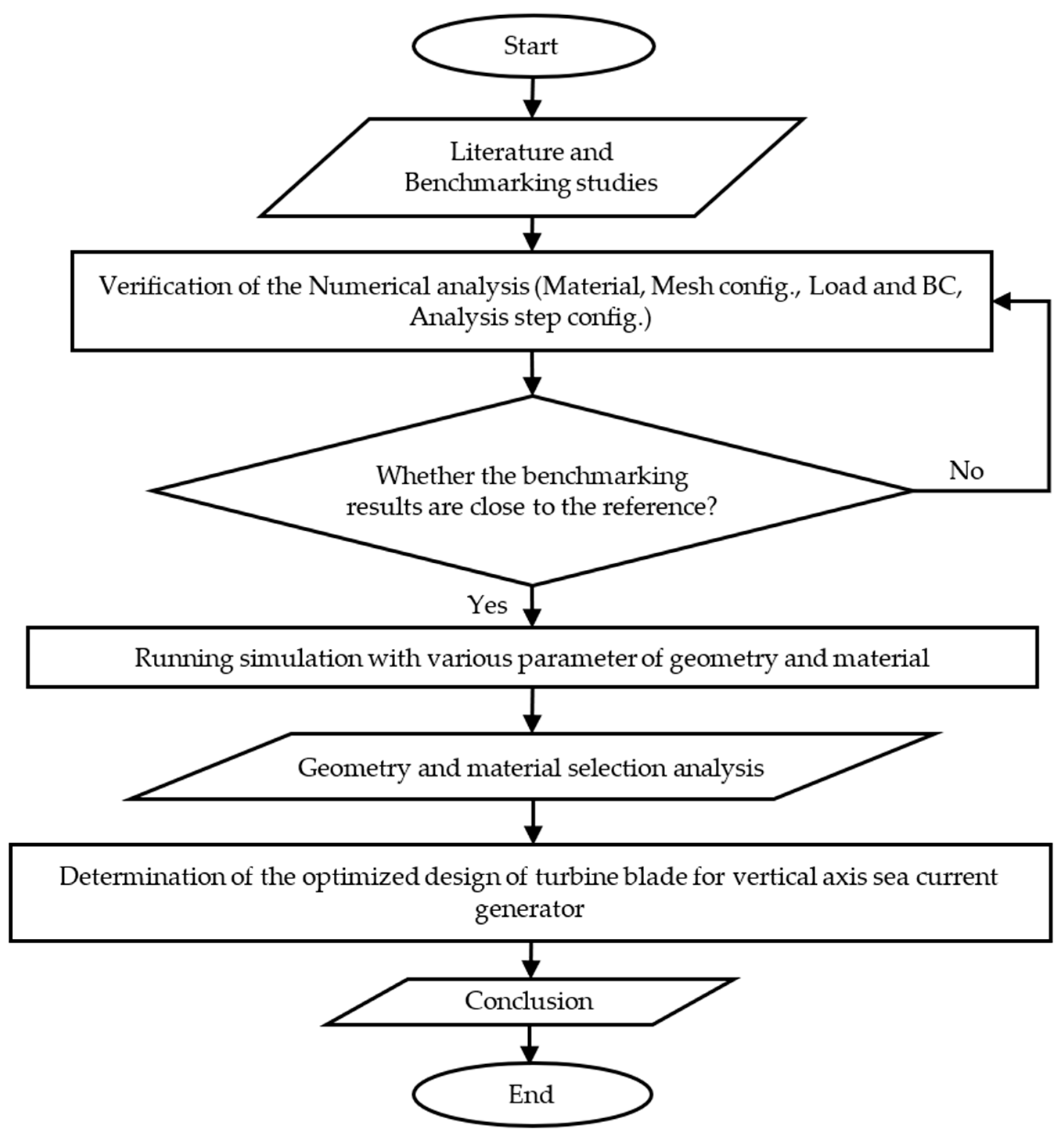
4.1. Flowchart

Because the method used in this research is a finite element method approach using ABAQUS CAE, there are several stages in conducting this research. The first is a literature study focused on the structure of turbine blades that have a vertical axis. After that, the studies conducted in previous research are replicated to validate the use of numerical methods. The results of the replication are compared with the reference; if it is close, then the research can continue. After that, various variations that have been determined previously are simulated and these results are analyzed. After completing the analysis, conclusions can be drawn. The flowchart of this research can be seen in Figure 6.

To assess the safety of a designed structure, such as an ocean current turbine blade, two approaches can be considered depending on the purpose: the ultimate limit state and the operational state. This manuscript focuses on the ultimate limit state capacity, aiming to investigate how structural parameters (material, supporting arm distance, framing system, and force direction) influence the ultimate strength of the blade through simulations using FEM. The operational state, using fluid–structure interaction (FSI) analysis, will be conducted in the near future to assess the safety factor.

4.2. Numerical Validation

Numerical validation was conducted by replicating the research on a vertical axis turbine conducted by Hameed and Afaq in 2013 [37]. The force control method was employed to obtain the ultimate capacity of the reaction force that can be handled by the structural system. The direction of the force is set to be perpendicular to the blade centerline to obtain the ultimate load response to the blade by imposing an idealized distributed load to model the drag force. This study focused on observing the load and deflection of the blade across several blade wall thicknesses.

The geometry that is used in the benchmarking study is a NACA 0015 blade with a total length of 2.58 m. Supports were placed at 0.56 m from each end. The material used in this study was aluminum with E = 70 GPa and v = 0.03 [38]. The boundary condition used in this validation study was an encase on each support so that all motion components were 0, and the loading given was a distributed load. The boundary condition and loading scheme are shown in Figure 7. Each wall thickness had a different loading magnitude.

Table 1. Loading value of each wall thickness.

Wall Thickness (mm)	Total Force (kN)
Solid	26.02
5	11.83
4	9.76
3	7.59

shows the value of the loading for each wall thickness.

In this benchmarking study, ABAQUS CAE 2023 software was employed using the General Statics step. The maximum displacement for each blade thickness was compared to assess the accuracy of the numerical settings used in this study. The outcomes of the benchmarking can be seen in

Table 2. Numerical validation results.

Wall Thickness (mm)	Deformation (mm)		Difference (%)
	Hameed and Afaq [37]	Current Study
Solid	7.39	7.90	6.9
5	4.51	4.76	5.5
4	4.27	3.99	6.5
3	4.07	3.93	3.4

and Figure 8.

The data in Table 2 reveal the discrepancies between this study and the research conducted by Hameed and Afaq, with an average difference of about 5.7%. The largest deviation was found in the solid blade, while the smallest difference occurred in blades with a wall thickness of 3 mm. This difference arises because of the different types of loading used. In this study, body force loading was used, while in the study conducted by Hameed and Afaq, a line load loading was used.

4.3. Numerical Modeling

The basic geometry used in this study is a turbine blade with a NACA 0021 airfoil profile [39]. The total length used in this study is 3600 mm, with varying distances between the supports. The geometry utilized in this study is depicted in Figure 9.

In the simulation of ocean currents, the load is modeled as a distributed load using a body force loading type. Each support is a fixed type support, thus $U_{x1}=U_{x2}=U_{y1}=U_{y2}=U_{z1}=U_{z2}={UR}_{x1}={UR}_{x2}={UR}_{y1}={UR}_{y2}={UR}_{z1}={UR}_{z2}$. The boundary condition and loading scheme are illustrated in Figure 10.

4.4. Mesh Convergence Study

A mesh convergence study is essential to determine a mesh size that balances accuracy with numerical efficiency [40]. This study was conducted by simulating the benchmarking model described in Section 4.1, featuring a distance between supports of 2000 mm and varying mesh sizes. The results of the mesh convergence study are displayed in Figure 11.

A straight line is drawn on the graph depicting the results of the mesh convergence study (Figure 11) to identify the convergence. In Figure 10, it is evident that a mesh size of 10 mm, corresponding to approximately 22,000 elements, is suitable. This is indicated by the observation that further reductions in mesh size do not significantly impact the results of the numerical calculations.

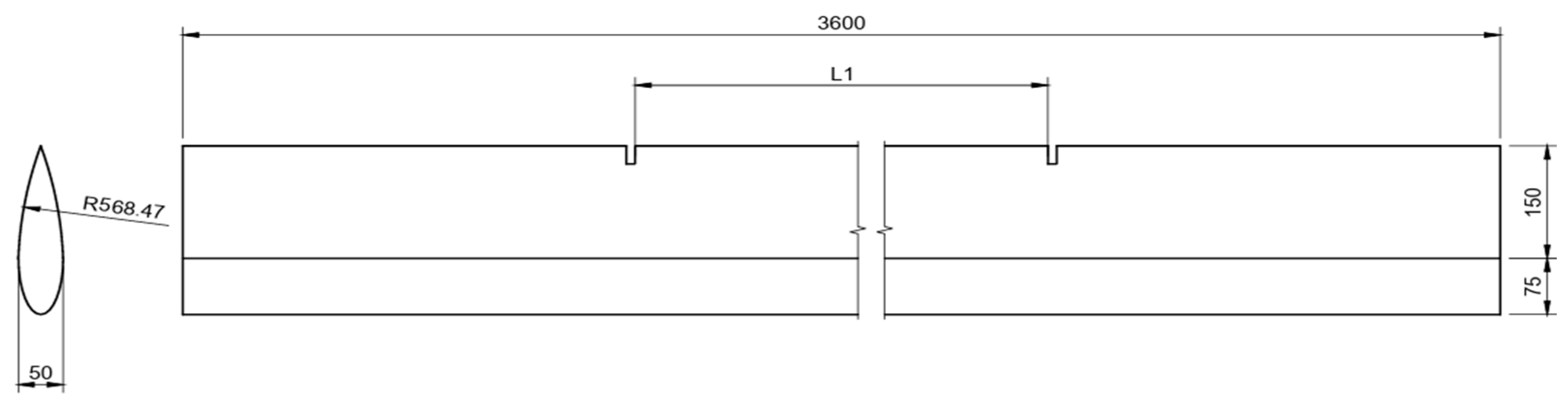
4.5. Space between Support Variation

Several variations in the distance between the supports were explored, with the supports positioned symmetrically to ensure an equal distance from each blade tip. In these variations, aluminum was used with a solid frame. Details of the space between supports are presented in

Table 3. Space between support variation.

Code	L1 (mm)	Distance from End (mm)
A-1	3600	0
A-2	3000	300
A-3	2800	400
A-4	2700	450
A-5	2500	550
A-6	2300	650
A-7	2200	700
A-8	2000	800
A-9	1600	1000
A-10	1000	1300
A-11	0	1800

.

4.6. Pitch Angle Variation

The pitch angle refers to the angle of the turbine blade relative to its axis, optimized to enhance hydrodynamics and achieve a high power coefficient (Cp) [41]. However, differences in pitch angle can affect the load on the turbine blade. Therefore, this study also examined how pitch angle influences the structural strength of the turbine blade. Because ABAQUS CAE cannot provide an angled force, the forces are analyzed in both the normal and tangential directions on the blade surface during simulations. Details of the pitch angle variations are listed in

Table 4. Pitch angle variation.

Code	Pitch Angle
B-1	−20°
B-2	−10°
B-3	−5°
B-4	0°
B-5	+5°
B-6	+10°
B-7	+20°

. In these variations, solid aluminum is used for the blade, with support configurations as in the case of A-8 and A-5.

4.7. Frame Variation

This study explored four frame model configurations. The first model features a bar frame, as depicted in Figure 12a. The second model is inspired by Wang et al.‘s research, which utilized a longitudinal web frame, shown in Figure 12b [42]. The third and fourth configurations involve a solid blade and a hollow blade without any stiffeners, respectively. The code for the frame shape variations can be seen in

Table 5. Frame shape variations.

Code	Frame Shape
C-1	Frame
C-2	Web
C-3	Solid Blade
C-4	Hollow Blade

.

4.8. Materials Variation

The material candidates were chosen for their suitability in marine environments, which are typically corrosive, while also possessing the necessary strength to withstand the applied loads. In this study, the materials evaluated included stainless steel, aluminum alloy 6061, and two types of fiber-reinforced plastic (FRP): carbon fiber-reinforced plastic (CFRP) [43] and glass fiber-reinforced plastic (GFRP). The variations and properties of these materials are detailed in

Table 6. Material variations.

Code	Material	Density (kg/m3)	Young’s Modulus (GPa)	Yield Strength (MPa)	Ultimate Strength (MPa)
D-1	Stainless Steel [44]	8000	193	539	766
D-2	Al 6061 [45]	2700	68.9	276	310
D-3	CFRP [46]	1800	130	1756	-
D-4	GFRP [47]	2500	45.6	1280	-

.

5. Result and Discussion

The analysis and discussion of the results focus on the maximum load, maximum displacement, and maximum stress for each configuration, using normalized values. The maximum load is normalized by the total weight of the blade, the maximum displacement by the blade’s total length (3600 mm), and the maximum stress by the yield strength of the material used. Additionally, there is a discussion of stress and displacement contours.

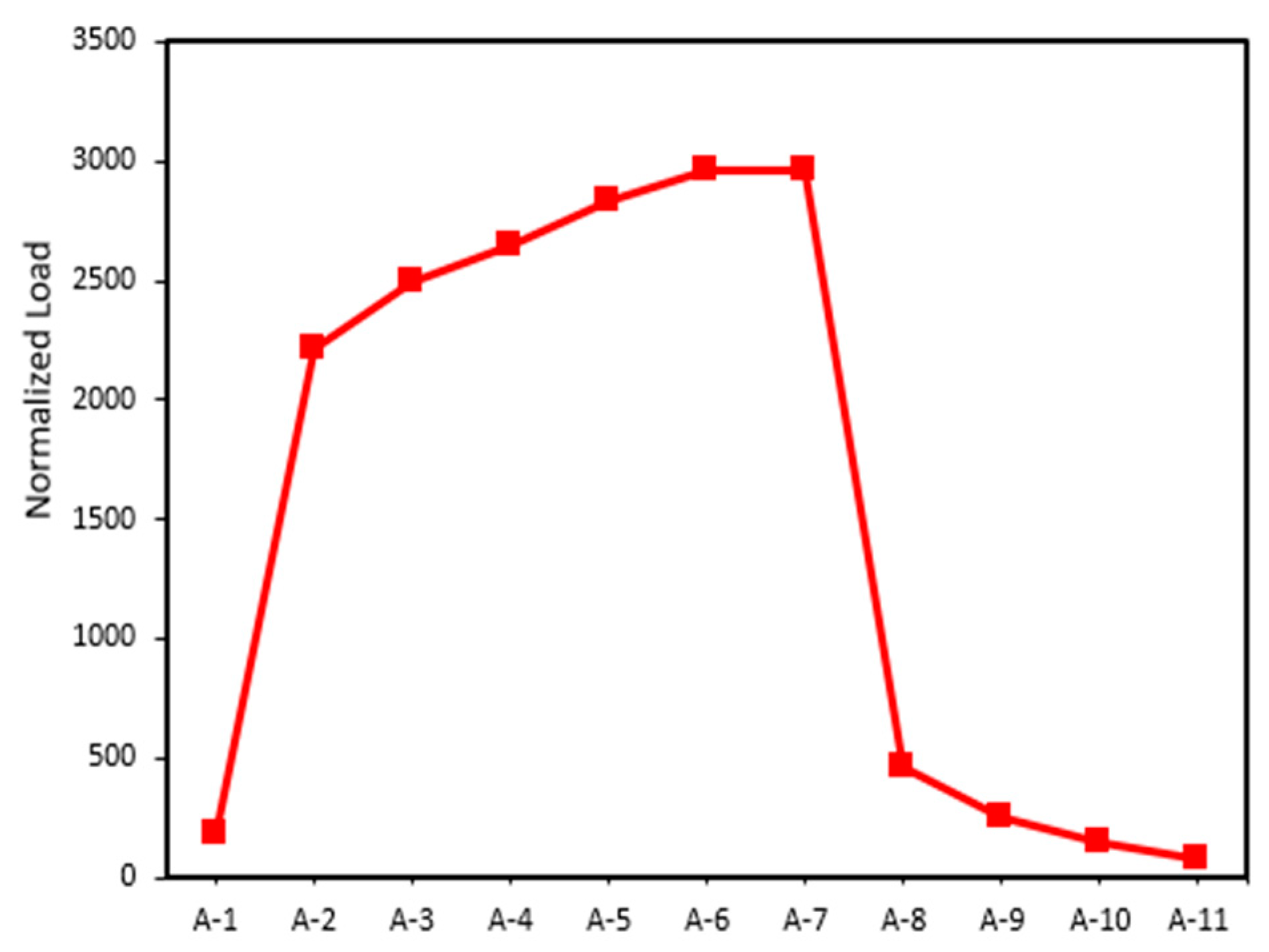
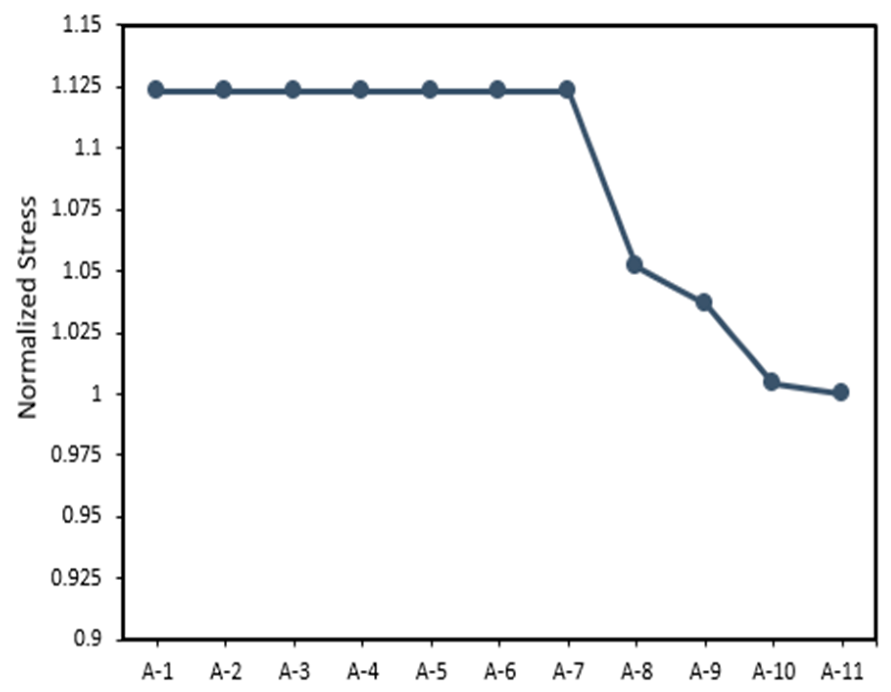
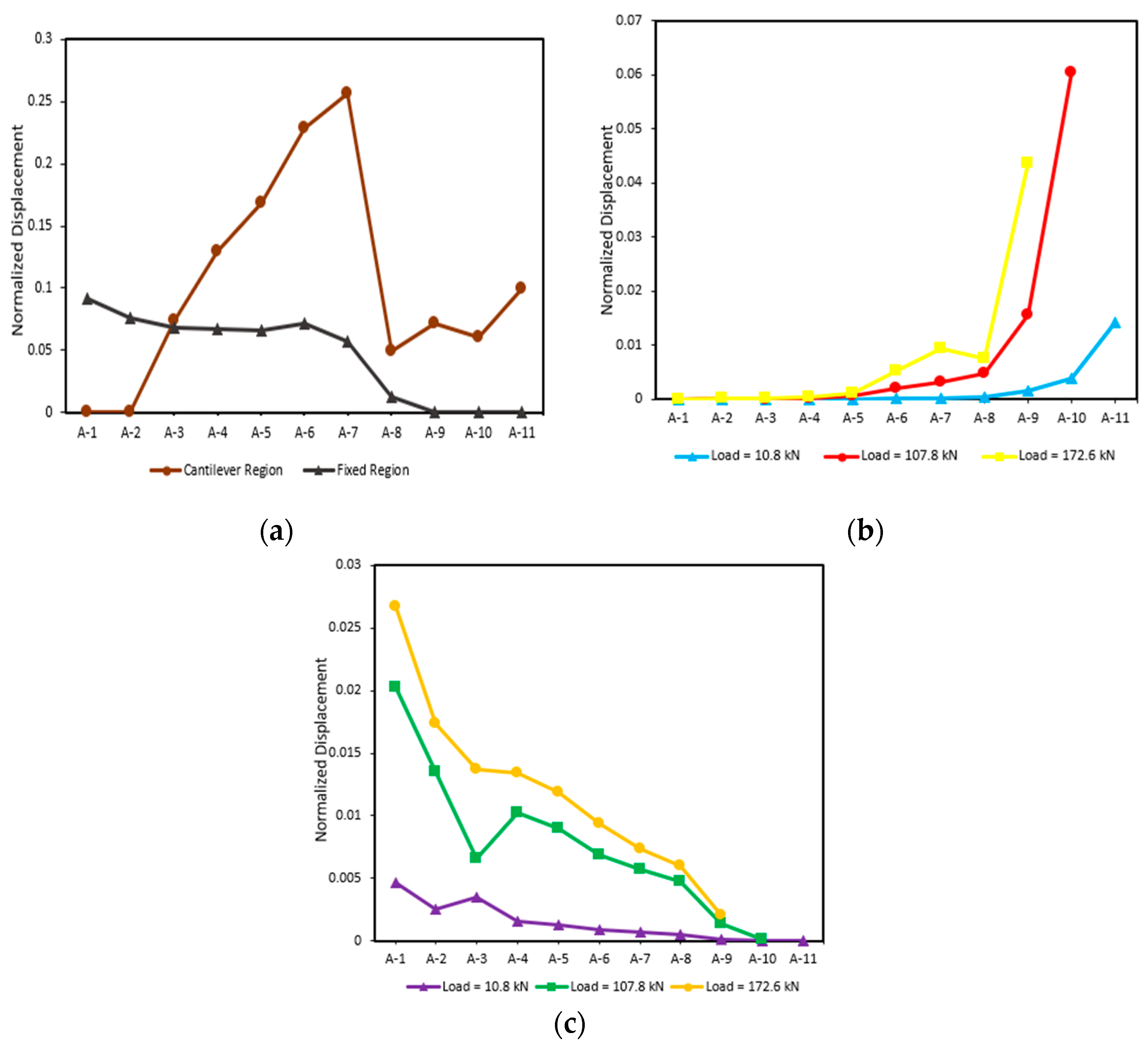
5.1. Space between Support

The results of the maximum load graph for each variation in the space between supports are displayed in Figure 13. These results are normalized by the total weight of the blade. An explanation of the variation code used can be seen in Table 3. Given that a solid aluminum blade is used, the actual load value has been normalized to 729 N.

In Figure 13, it is evident that configurations A-2 to A-7 display high maximum load values, while A-8 shows a substantial drop from A-7, a change further explored in the stress contours shown in Figure 14. After A-8, the maximum load will continue to decrease as it approaches the center of the blade. This decrease is attributed to the increase in moment load in the cantilever region when the support moves closer to the center of the blade. Whereas before A-7, the maximum load will decrease as the distance between the supports increases, which is also due to the increased moment in the fixed region as the support moves away from the center of the blade. The drop in maximum load that occurs between A-7 and A-8 is because at A-1 to A-7, the stress distribution is more evenly distributed along the blade. Whereas in A8 to A-11, the maximum stress occurs only where the supports are placed triggering local failures. Therefore, the optimal placement for the support, based on maximum load considerations, is at positions A-6 and A-7.

The maximum stress graph is normalized by the yield strength of aluminum because aluminum is the material used in this variation. Therefore, the maximum stress is normalized to 276 MPa. The maximum stress graphs and stress contours for several variations are displayed in Figure 14 and Figure 15.

In Figure 14, it can be observed that the maximum stress value remains constant when the support is positioned from A-1 to A-7. However, after passing A-7, the maximum stress value drops and follows a decreasing trend. This occurs because from A-1 to A-7, the stress distribution can fulfill the entire fixed region (as shown in Figure 15a,b). In contrast, from A-8 to A-11, the stress distribution is concentrated only where the support is placed. Consequently, A-1 to A-7 can withstand more load compared to A-8 to A-11 because the stress is more evenly distributed. The progression of stress for each variation is almost identical, where the highest stress initially appears at the support location and then spreads throughout the turbine blade.

Figure 16 depicts the maximum displacement and displacement at various loads in both the cantilever region and fixed regions. The displacement graphs are normalized by the total length of the turbine blade, which is 3600 mm. Additionally, Figure 16 provides a contour representation of the maximum displacement for several variations.

In Figure 16b, it can be seen that in the cantilever region, the closer the distance between the supports, the higher the displacement will be. Conversely, Figure 17c shows that the further the support distance from the center of the blade, the higher the displacement in the fixed region. This is because, in the cantilever region, the load increases when the support is closer to the center of the blade, leading to increased displacement. Conversely, the further the support is from the center of the blade, the greater the load in the cantilever region, as also depicted in the displacement contours shown in Figure 17.

However, in Figure 16a, it can be seen that the maximum displacement in the cantilever region from A-4 to A-7 is higher when compared to A-8 to A-11. This is because A-4 to A-7 can withstand a higher load, resulting in a greater maximum displacement, as shown in Figure 13. Since displacement is directly proportional to load (Equation (1)), the higher the load that can be received, the greater the displacement.

When considering the maximum load, maximum stress, maximum displacement, and the stress and displacement contours, it is evident that support is most effective when used in geometry A-7. This is because geometry A-7 exhibits the highest values for maximum load, stress, and displacement compared to other geometries where the support might be placed.

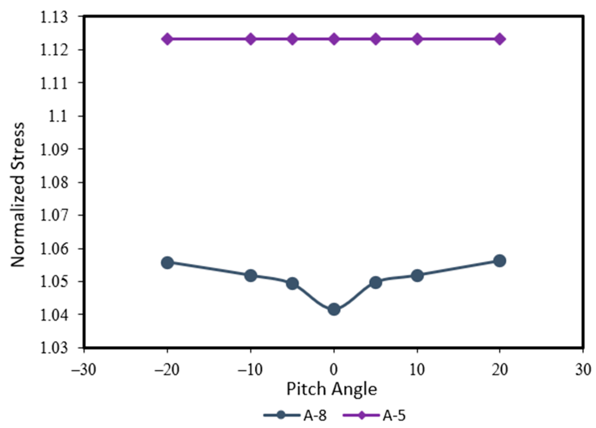
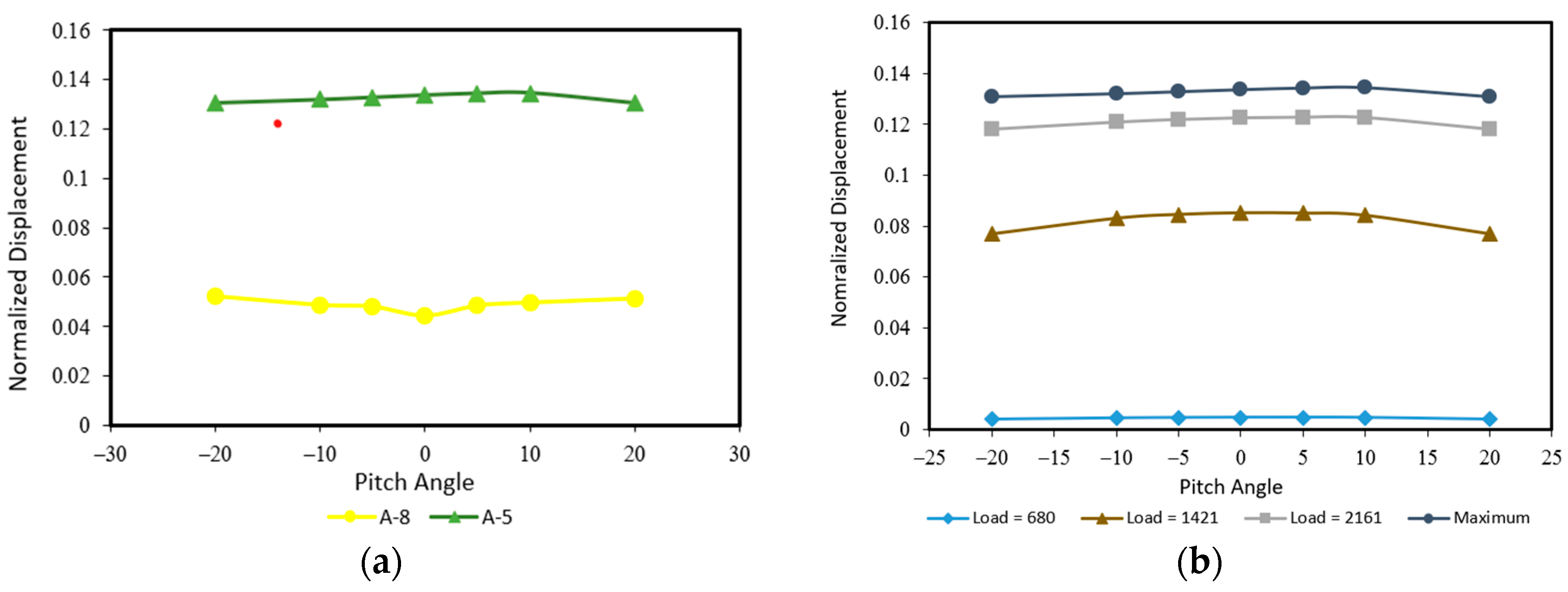
5.2. Pitch Angle

The results from the maximum load graph, based on the variation of pitch angle, are presented in Figure 18. Figure 18a shows the maximum load for each load component, while Figure 18b displays the total maximum load. The results are normalized by the total weight of the blade. Since a solid aluminum blade is utilized, the actual load value is normalized to 729 N. An explanation of the variation code used can be seen in Table 3.

In Figure 18b, it can be observed that the total maximum load is unaffected by the pitch angle. This observation is supported by Figure 18a, where the maximum load on the X-component is significantly smaller compared to that on the Z-component. However, as the pitch angle increases in both negative and positive directions, the maximum load in the X-component rises, leading to a decrease in the maximum load on the Z-component. The placement of the support also influences the effect of pitch angle. This is demonstrated in Figure 18a, where the maximum load slope gradient on the X-component is lower when the support is positioned at A-8 compared to A-5. This is due to the higher maximum load on support A-5 compared to A-8, as discussed in Section 5.1.

Figure 19 displays the maximum stress graph for each pitch angle, while Figure 20 illustrates the stress contours for several pitch angles with the support positioned at A-8. In Figure 20, the maximum stress is normalized to 276 MPa, reflecting the properties of the solid aluminum material used in the blade.

The resulting maximum stress indicates that when the support is positioned at A-5, it yields a higher value than when placed at A-8, as shown in the graph in Figure 19. This is consistent with the discussion in Section 4.1, where it is noted that A-5 has a more even stress distribution compared to A-8. The stress contours displayed in Figure 20 show minimal variation between different pitch angles, with the maximum stress localized at the support only. This occurs because the load in the Z direction is still significantly greater than that in the X direction, resulting in similar stress contours across variations.

As with the previous displacement graph, the displacement value is normalized by the length of the entire blade, which is 3600 mm. Since the support is positioned at A-5 and A-8, the maximum displacement occurs in the cantilever region, and thus, the displacement shown is the maximum displacement of the cantilever region. Figure 21 presents the displacement graph, and Figure 22 shows the displacement contours at A-8.

As discussed in Section 4.1, positioning the support at A-5 results in higher displacement compared to when it is placed at A-8. This occurs because the support at A-5 bears a higher maximum load. This is further illustrated in Figure 21a, where the support at A-5 exhibits a higher maximum displacement than the support at A-8.

Meanwhile, the magnitude of the pitch angle does not significantly affect the maximum displacement produced. This can be seen in Figure 21b and Figure 22. This is because the maximum load, as shown in Figure 18, does not vary greatly between different pitch angles, so the maximum displacement that appears also does not have a big effect either.

Considering factors previously discussed, such as maximum load, displacement, and stress, it is evident that the magnitude of the pitch angle does not significantly affect the structural integrity of the blade. Therefore, regardless of the hydrodynamics produced by each pitch angle, any pitch angle is suitable for use.

5.3. Frame Geometry

In the analysis of frame geometry variations, each load is normalized by its weight. As each geometry possesses a distinct volume, the normalization differs accordingly. This process enables the comparison of strength-to-weight ratios across different geometries.

Table 7. Normalized value for each geometry.

Code	Normalized by (N)
C-1 (frame)	237.6
C-2 (web)	150.2
C-3 (solid)	129.6
C-4 (hollow)	729.0

displays the normalized loads for each geometry. An explanation of the variation code used can be seen in Table 5. The illustration of the frame and web design used can be seen in Figure 12. Figure 23a shows the maximum loads before normalization, whereas Figure 23b presents the normalized values.

Figure 23a shows that, in terms of maximum load, C-4 possesses the greatest strength, followed by C-1, C-2, and finally, C-3. The superior strength of C-4 can be attributed to its solid blade design, which features a larger cross-sectional area. This larger area allows for improved stress distribution across the cross-section, enabling it to support heavier loads. Conversely, the hollow blades have a smaller cross-sectional area, making them more prone to failure under high loads.

Figure 23b reveals that when the maximum load is normalized by the weight of each frame geometry variation, C-2 displays the highest normalized load, followed by C-3, C-1, and C-4. This indicates that the maximum load-to-weight ratio for web design is highly efficient, resulting in a substantial normalized load value.

The maximum stress, normalized to the yield strength of aluminum, remains consistent with the parameters discussed previously, as aluminum is still the material in use. Consequently, the maximum stress is normalized to 276 MPa. Figure 24 presents the graph of maximum stress for the frame geometries, while Figure 25 displays the stress contours for several frame geometries.

In Figure 24, it can be observed that as the blade becomes more solid, the maximum stress also increases. This is due to the fact that a more solid blade’s cross-sectional area can distribute the load more effectively. Figure 25a–c demonstrate a better stress distribution compared to Figure 22c because the geometries C-1, C-2, and C-3 have a wider area of maximum stress compared to geometry C-4, as indicated by the larger, red-colored area on the contour.

Since this geometry variation maintains the same total blade length, the displacement value is normalized to 3600 mm. Figure 26 presents a graph of displacement under various loads, along with the maximum displacement value for each geometry. Meanwhile, Figure 25 shows the displacement contour for each frame geometry used.

Figure 26 shows that at the same load, blade geometries with many voids exhibit larger displacements compared to more solid blade geometries. This occurs because a more solid blade has higher stiffness, resulting in less displacement under the same load, as indicated in Equation 7. However, the maximum displacement of the more solid blade is higher, as seen in Figure 26. This is attributed to the higher maximum load that the solid blade can withstand, as shown in Figure 24, leading to greater maximum displacement.

In Figure 27, it is evident that geometries C-1, C-2, and C-3 exhibit similar displacement contours, indicating that the blade can bend, even though geometries C-1 and C-2 are not solid blades. This is because geometries C-1 and C-2 have reinforcements running along the blade, preventing the edges from collapsing under load. In contrast, geometry C-4 shows flaking at the end of the blade.

Based on the previous discussion, it can be concluded that the most suitable frame geometry for the turbine blade frame of an ocean current power generator is the C-2 geometry. Despite having a small maximum displacement and a relatively high maximum load, this geometry exhibits an excellent load-to-weight ratio compared to other geometries. 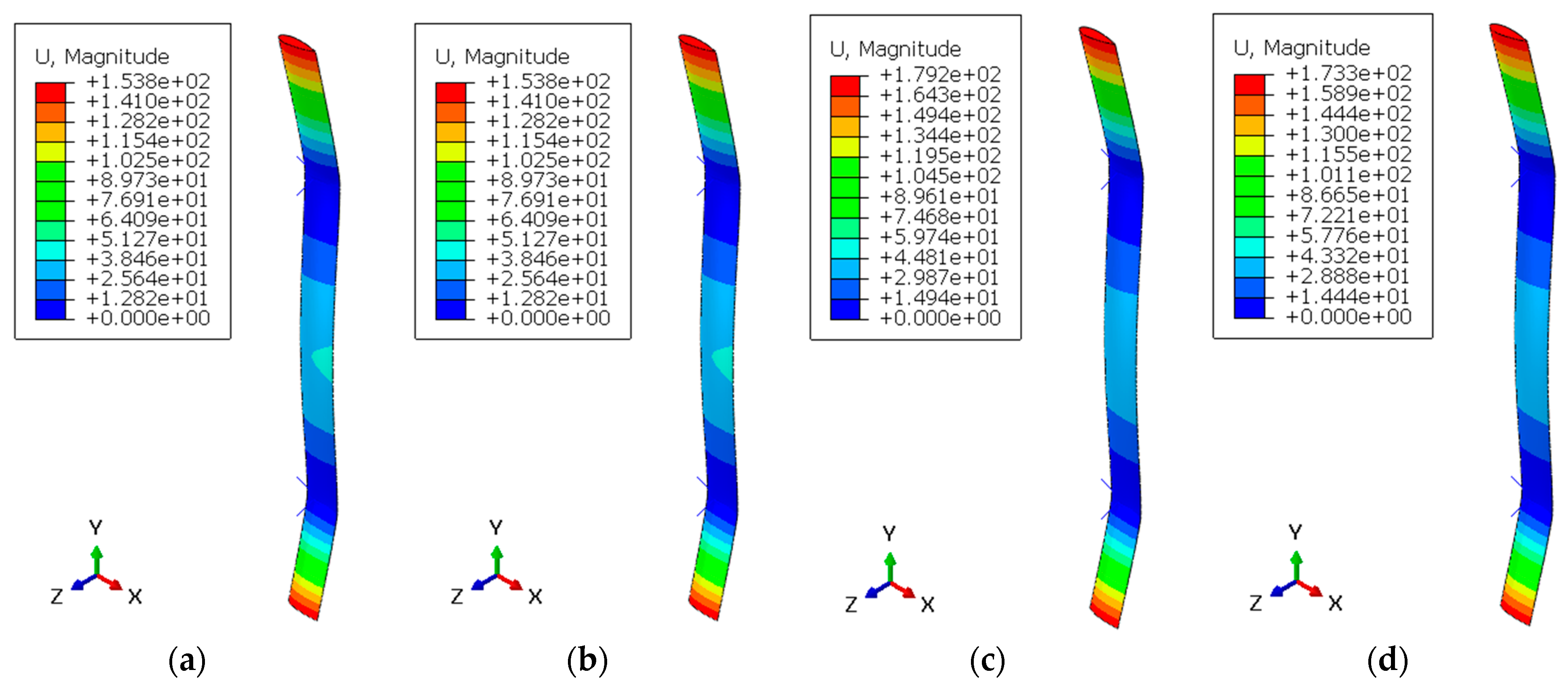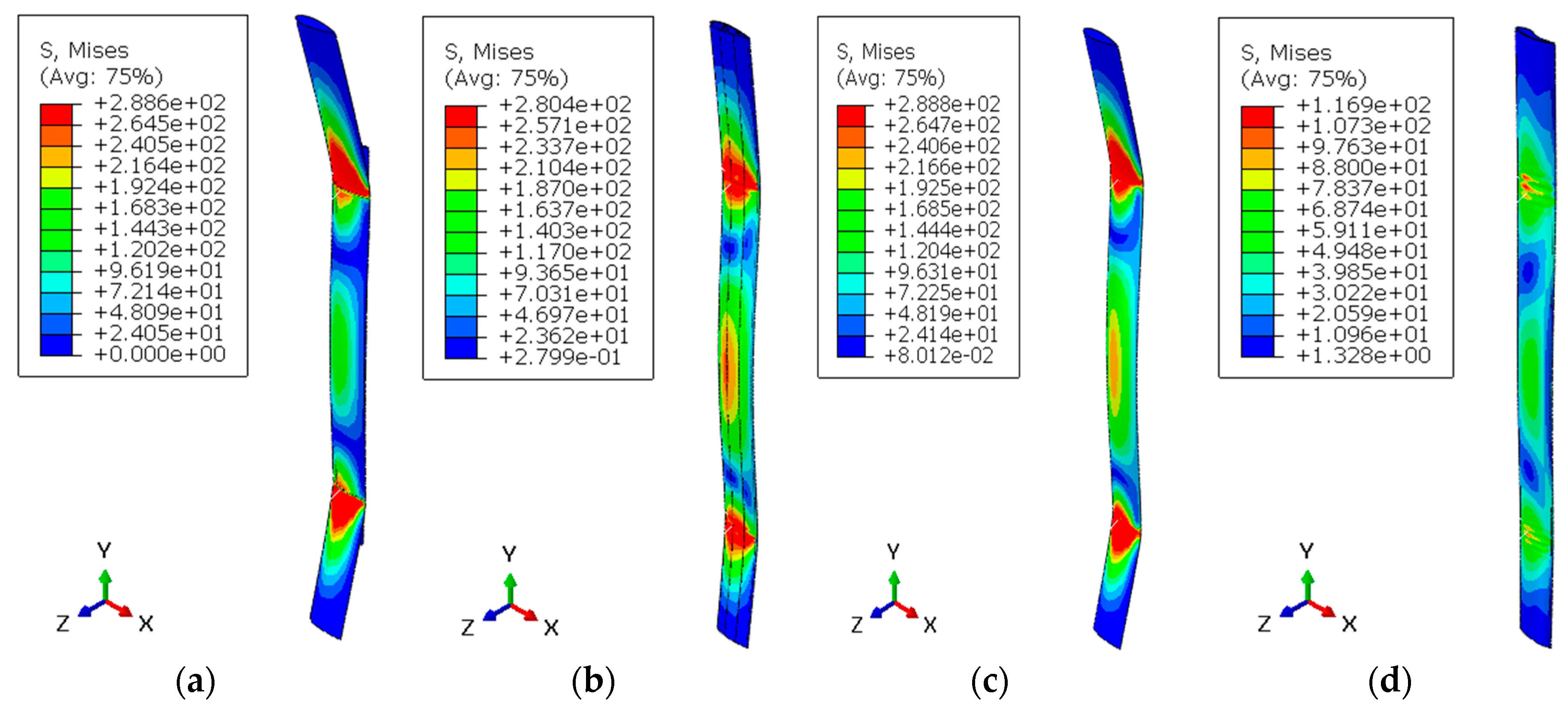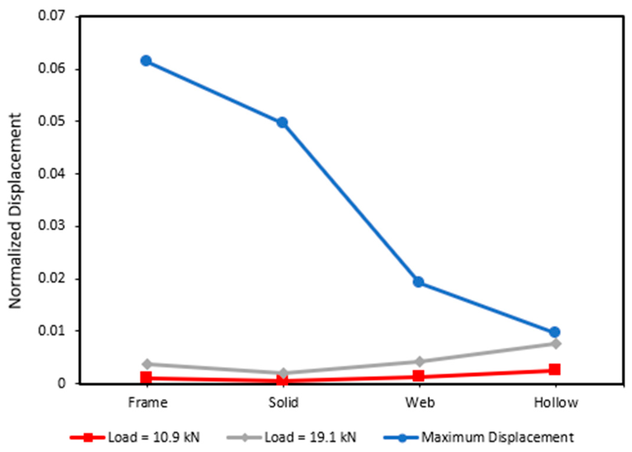Additionally, the maximum stress experienced by this geometry is comparable to that of the more rigid blade geometry.

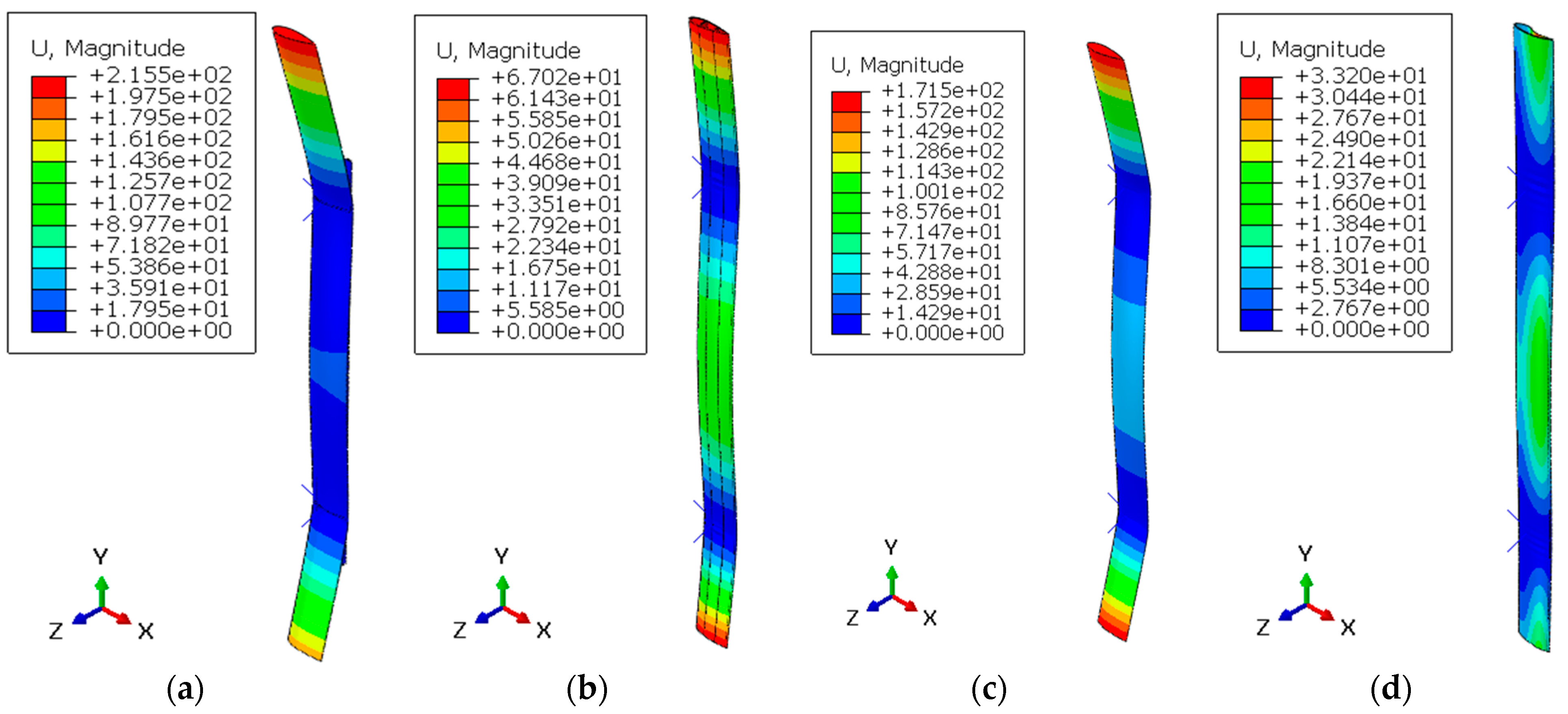
5.4. Material

Since these variations use different materials and include both solid and hollow blades, the maximum load is normalized to different values. However, normalization is still performed based on the weight of each variation. The normalized values for each variation are presented in

Table 8. Normalized value for each material variation.

Code	Normalized by (N)
	Hollow Blade	Solid Blade
D-1 (Stainless Steel)	384.0	2160
D-2 (Aluminum)	129.6	729
D-3 (CFRP)	86.4	486
D-4 (GFRP)	120.0	675

. An explanation of the variation code used can be seen in Table 6. Additionally, there are two graphs associated with this variation: Figure 28a shows the true maximum load graph for each variation, while Figure 28b displays the normalized maximum load graph.

In Figure 28a, it is evident that material D-1 has the highest maximum load, followed by D-3, and then D-4, with D-2 having the smallest maximum load. The difference in maximum load for each material is attributed to the varying values of yield strength and ultimate strength of each material. This phenomenon is observed in both types of blades used.

However, due to the high density of the D-1 material compared to the other materials, its maximum load-to-weight ratio is relatively low. This is illustrated in Figure 28b, where the composite material exhibits a higher maximum load-to-weight ratio than the metallic material. This occurs because the composite material is lighter than the metallic material.

Since the materials used in this variation are different, the normalized stress value in the maximum stress graph for each variation also differs. The yield strength of each material is shown in Table 6. Figure 29 presents the maximum stress graph normalized by the yield strength of each variation, while Figure 30 displays the stress contours of the material variations used.

Figure 29 shows that the metallic material has a maximum stress that exceeds its yield strength. This is because metallic materials have a plastic region, allowing the stress to exceed the yield strength of the material. However, when not normalized, the composite material exhibits a higher failure stress compared to the metallic material. This is illustrated in Figure 30, where the D-3 and D-4 materials reach 1756 MPa and 1280 MPa, respectively. The higher failure stress is due to the higher ultimate strength of the composite material compared to the metallic material, as shown in Table 6.

Since the total blade length remains unchanged in this variation, the displacement graph is normalized to 3600 mm. Figure 31 presents a graph of maximum displacement and displacement at various loads, while Figure 32 shows the displacement contour for each variation.

In Figure 31, it is evident that the displacement generated by each material variation under the same load is different. This difference is due to the varying values of Young’s Modulus in each material. A higher Young’s Modulus indicates a stiffer material; thus, in Figure 31, material D-3 has the smallest displacement under the same load. However, the maximum load that a material can withstand also affects the maximum displacement produced. Consequently, at the point of maximum displacement, material D-1 exhibits the largest maximum displacement.

From the earlier discussion, it can be concluded that the best material for turbine blades in ocean current power generator applications is the D-3 material. Despite having a small maximum displacement, this material exhibits an excellent maximum load-to-weight ratio and has a high failure stress.

6. Conclusions

From the simulations that have been carried out, the following can be concluded:

• The optimal distance between supports for the turbine blade in an ocean current power generator is 2200 mm. This distance provides the most optimal load distribution, resulting in an even distribution of stress. The even stress distribution allows this support distance to achieve a high maximum load and, consequently, a high maximum displacement.
• A pitch angle between −20° and 20° does not significantly affect the structural strength of a turbine blade. This is because the load on the axial component of the blade is much smaller than the load on the normal component. Therefore, as long as the aerodynamics of the blade are not considered, the pitch angle can be freely adjusted within this range.
• The frame geometry used in turbine blades affects rigidity, weight, and blade surface area. This variation causes the maximum load, stress, displacement, and maximum load-to-weight ratio to differ for each geometry. The more solid a blade frame is, the higher the maximum load, stress, and displacement due to better stress distribution. However, a more solid frame results in a smaller maximum load-to-weight ratio. Therefore, a blade-shaped frame is chosen because it offers the best maximum load-to-weight ratio among the various frame shapes.
• Each material has different mechanical properties. The higher ultimate strength of a material increases the maximum stress it can withstand. A higher Young’s Modulus increases the blade stiffness, thereby reducing the displacement. However, a higher material density increases the blade weight, reducing the maximum load-to-weight ratio. Therefore, CFRP material is selected because it offers a high maximum load-to-weight ratio and can withstand high maximum stress.

Recommendations suggested for further research are to pay attention to the impact of total weight on the hydrodynamic forces to ensure that the selected material and frame are efficient in generating hydrodynamic force that may affect power output. In addition, this parametric study is limited to the numerical analysis assessing the influence of structural parameters on the ultimate capacity as a preliminary design, which can be used as a guide to improve the structural capacity for the desired safety factor. For future studies, the fluid–solid interaction (FSI) problem will be considered to portray the operational loading capacity and obtain the safety factor after being compared with the ultimate one.

References

- Farmer, G.T.; Cook, J. The World Ocean BT—Climate Change Science: A Modern Synthesis: Volume 1—The Physical Climate; Farmer, G.T., Cook, J., Eds.; Springer: Dordrecht, The Netherlands, 2013; pp. 247–259. [Google Scholar] [CrossRef]
- Adie, P.W.; Adiputra, R.; Prabowo, A.R.; Erwandi, E.; Muttaqie, T.; Muhayat, N.; Huda, N. Assessment of the OTEC cold water pipe design under bending loading: A benchmarking and parametric study using finite element approach. J. Mech. Behav. Mater. 2023, 32, 20220298. [Google Scholar] [CrossRef]
- Chen, H.; Zhang, X.; Xu, Y. Modeling, simulation, and experiment of switched reluctance ocean current generator system. Adv. Mech. Eng. 2013, 2013, 5. [Google Scholar] [CrossRef]
- Madi, M.; Mukhtasor; Rahmawati, S.; Satrio, D.; Tuswan, T.; Ismail, A. Experimental Study on the Effect of Single Flow Disturber on the Performance of the Straight-Bladed Hydrokinetic Turbine at Low Current Speed. Pomorstvo 2024, 38, 43–54. [Google Scholar] [CrossRef]
- Madi, M.; Mukhtasor, M.; Satrio, D.; Tuswan, T.; Ismail, A.; Rafi, R.; Yunesti, P.; Buana, S.W.; Jarwinda, J. Experimental Study on the Effect of Foil Guide Vane on the Performance of a Straight-Blade Vertical Axis Ocean Current Turbine. Nase More 2024, 71, 1–11. [Google Scholar] [CrossRef]
- Chiang, H.W.D.; Lin, C.Y.; Hsu, C.N. Design and performance study of an ocean current turbine generator. Int. J. Turbo Jet Engines 2013, 30, 293–302. [Google Scholar] [CrossRef]
- Fizari, A.J.; Wijaya, F.D.; Cahyadi, A.I.; Adiyasa, I.W. Design and Simulation Permanent Magnet Synchronous Generator 1.5 kW for Ocean Current Turbine. In Proceedings of the CENCON 2019—2019 IEEE Conference on Energy Conversion (CENCON), Yogyakarta, Indonesia, 16–17 October 2019. [Google Scholar] [CrossRef]
- Tian, W.; Ni, X.; Mao, Z.; Zhang, T. Influence of surface waves on the hydrodynamic performance of a horizontal axis ocean current turbine. Renew. Energy 2020, 158, 37–48. [Google Scholar] [CrossRef]
- Mubarok, M.A.; Arini, N.R.; Satrio, D. Optimization of Horizontal Axis Tidal Turbines Farming Configuration Using Particle Swarm Optimization (PSO) Algorithm. In Proceedings of the 2023 International Electronics Symposium (IES), Denpasar, Indonesia, 8–10 August 2023. [Google Scholar] [CrossRef]
- Ng, K.W.; Lam, W.H.; Ng, K.C. 2002–2012: 10 Years of Research Progress in Horizontal-Axis Marine Current Turbines. Energies 2013, 6, 1497–1526. [Google Scholar] [CrossRef]
- Sasmita, A.F.; Arini, N.R.; Satrio, D. Numerical Analysis of Vertical Axis Tidal Turbine: A Comparison of Darrieus and Gorlov Type. In Proceedings of the 2023 International Electronics Symposium (IES), Denpasar, Indonesia, 8–10 August 2023. [Google Scholar] [CrossRef]
- Akimoto, H.; Tanaka, K.; Uzawa, K. A conceptual study of floating axis water current turbine for low-cost energy capturing from river, tide and ocean currents. Renew. Energy 2013, 57, 283–288. [Google Scholar] [CrossRef]
- Erwandi, E.; Kasharjanto, A.; Satrio, D.; Rahuna, D.; Suyanto, E.M.; Mintarso, C.S.J.; Irawanto, Z.; Ramadhani, M.A. Numerical Analysis of Resistance and Motions on Trimaran Floating Platform for Tidal Current Power Plant. Int. Rev. Model. Simul. 2024, 17, 6–16. [Google Scholar] [CrossRef]
- Zhou, Z.; Benbouzid, M.; Charpentier, J.F.; Scuiller, F.; Tang, T. Developments in large marine current turbine technologies—A review. Renew. Sustain. Energy Rev. 2017, 71, 852–858. [Google Scholar] [CrossRef]
- Xie, J.; Chen, J. Vertical-axis ocean current turbine design research based on separate design concept. Ocean Eng. 2019, 188, 106258. [Google Scholar] [CrossRef]
- Zeiner-Gundersen, D.H. A novel flexible foil vertical axis turbine for river, ocean, and tidal applications. Appl. Energy 2015, 151, 60–66. [Google Scholar] [CrossRef]
- Nguyen, M.T.; Balduzzi, F.; Goude, A. Effect of pitch angle on power and hydrodynamics of a vertical axis turbine. Ocean Eng. 2021, 238, 109335. [Google Scholar] [CrossRef]
- Hasankhani, A.; VanZwieten, J.; Tang, Y.; Dunlap, B.; De Luera, A.; Sultan, C.; Xiros, N. Modeling and numerical simulation of a buoyancy controlled ocean current turbine. Int. Mar. Energy J. 2021, 4, 47–58. [Google Scholar] [CrossRef]
- Chen, J.H.; Wang, X.C.; Li, H.; Jiang, C.H.; Bao, L.J. Design of the blade under low flow velocity for horizontal axis tidal current turbine. J. Mar. Sci. Eng. 2020, 8, 989. [Google Scholar] [CrossRef]
- Wang, H.-M.; Qu, X.-K.; Chen, L.; Tu, L.-Q.; Wu, Q.-R. Numerical study on energy-converging efficiency of the ducts of vertical axis tidal current turbine in restricted water. Ocean Eng. 2020, 210, 107320. [Google Scholar] [CrossRef]
- Satrio, D.; Suntoyo; Widyawan, H.B.; Ramadhani, M.A.; Muharja, M. Effects of the distance ratio of circular flow disturbance on vertical-axis turbine performance: An experimental and numerical study. Sustain. Energy Technol. Assess. 2024, 63, 103635. [Google Scholar] [CrossRef]
- Rahuna, D.; Erwandi; Satrio, D.; Utama, I.K.A.P. Opportunities for Utilizing Vortex Generators on Vertical Axis Ocean Current Turbines: A Review. BIO Web Conf. 2024, 89, 10003. [Google Scholar] [CrossRef]
- Hatoro, R.; Utama, I.K.A.P.; Erwandi, E.; Sulistyono, A. An Experimental Investigation of passive Variable-pitch Vertical Axis Ocean Current Turbine. J. Eng. Technol. Sci. 2011, 43, 27–40. [Google Scholar] [CrossRef]
- Liu, T. Evolutionary understanding of airfoil lift. Adv. Aerodyn. 2021, 3, 37. [Google Scholar] [CrossRef]
- Bora, M.; Sharma, A.V.; Kumari, P.; Sahoo, N. Investigation of bamboo-based vertical axis wind turbine blade under static loading. Ocean. Eng. 2023, 285, 115317. [Google Scholar] [CrossRef]
- Patel, V.; Rathod, V.; Patel, C. Optimal utilization of hydrokinetic energy resources through performance improvement of the darrieus turbine using concave and flat blocking plates. Ocean Eng. 2023, 283, 115099. [Google Scholar] [CrossRef]
- Asadbeigi, M.; Ghafoorian, F.; Mehrpooya, M.; Chegini, S.; Jarrahian, A. A 3D Study of the Darrieus Wind Turbine with Auxiliary Blades and Economic Analysis Based on an Optimal Design from a Parametric Investigation. Sustainability 2023, 15, 4684. [Google Scholar] [CrossRef]
- Patel, V.; Eldho, T.I.; Prabhu, S.V. Performance enhancement of a Darrieus hydrokinetic turbine with the blocking of a specific flow region for optimum use of hydropower. Renew. Energy 2019, 135, 1144–1156. [Google Scholar] [CrossRef]
- Li, Z.; Xu, H.; Feng, J.; Chen, H.; Kan, K.; Li, T.; Shen, L. Fluctuation characteristics induced by energetic coherent structures in air-core vortex: The most complex vortex in the tidal power station intake system. Energy 2024, 288, 129778. [Google Scholar] [CrossRef]
- Ainsworth, M.; Parker, C. Unlocking the secrets of locking: Finite element analysis in planar linear elasticity. Comput. Methods Appl. Mech. Eng. 2022, 395, 115034. [Google Scholar] [CrossRef]
- Cascio, I.; Milazzo, M.L.; Benedetti, A. Virtual element method for computational homogenization of composite and heterogeneous materials. Compos. Struct. 2020, 232, 111523. [Google Scholar] [CrossRef]
- Anderson, R.; Andrej, J.; Barker, A.; Bramwell, J.; Camier, J.-S.; Cerveny, J.; Dobrev, V.; Dudouit, Y.; Fisher, A.; Kolev, T.; et al. MFEM: A modular finite element methods library. Comput. Math. Appl. 2021, 81, 42–74. [Google Scholar] [CrossRef]
- Genao, F.Y.; Kim, J.; Żur, K.K. Nonlinear finite element analysis of temperature-dependent functionally graded porous micro-plates under thermal and mechanical loads. Compos. Struct. 2021, 256, 112931. [Google Scholar] [CrossRef]
- Hartmann, S. A remark on the application of the Newton-Raphson method in non-linear finite element analysis. Comput. Mech. 2005, 36, 100–116. [Google Scholar] [CrossRef]
- Pho, K.H. Improvements of the Newton–Raphson method. J. Comput. Appl. Math. 2022, 408, 114106. [Google Scholar] [CrossRef]
- Zhang, A.; Mohr, D. Using neural networks to represent von Mises plasticity with isotropic hardening. Int. J. Plast. 2020, 132, 102732. [Google Scholar] [CrossRef]
- Hameed, M.S.; Afaq, S.K. Design and analysis of a straight bladed vertical axis wind turbine blade using analytical and numerical techniques. Ocean Eng. 2013, 57, 248–255. [Google Scholar] [CrossRef]
- Ponnusamy, P.; Rashid, R.A.R.; Masood, S.H.; Ruan, D.; Palanisamy, S. Mechanical properties of slm-printed aluminium alloys: A review. Materials 2020, 13, 4301. [Google Scholar] [CrossRef]
- Holst, D.; Church, B.; Wegner, F.; Pechlivanoglou, G.; Nayeri, C.N.; Paschereit, C.O. Experimental Analysis of a NACA 0021 Airfoil under Dynamic Angle of Attack Variation and Low Reynolds Numbers. J. Eng. Gas Turbine Power 2019, 141, 031020. [Google Scholar] [CrossRef]
- Adie, P.W.; Prabowo, A.R.; Muttaqie, T.; Adiputra, R.; Muhayat, N.; Carvalho, H.; Huda, N. Non-linear assessment of cold water pipe (CWP) on the ocean thermal energy conversion (OTEC) installation under bending load. Procedia Struct. Integr. 2023, 47, 142–149. [Google Scholar] [CrossRef]
- Ardaneh, F.; Abdolahifar, A.; Karimian, S.M.H. Numerical analysis of the pitch angle effect on the performance improvement and flow characteristics of the 3-PB Darrieus vertical axis wind turbine. Energy 2022, 239, 122339. [Google Scholar] [CrossRef]
- Wang, L.; Kolios, A.; Nishino, T.; Delafin, P.L.; Bird, T. Structural optimisation of vertical-axis wind turbine composite blades based on finite element analysis and genetic algorithm. Compos. Struct. 2016, 153, 123–138. [Google Scholar] [CrossRef]
- Satrio, D.; Musabikha, S.; Junianto, S.; Prifiharni, S.; Kusumastuti, R.; Nikitasari, A.; Priyotomo, G. The Advantages and Challenges of Carbon Fiber Reinforced Polymers for Tidal Current Turbine Systems—An Overview. In IOP Conference Series: Earth and Environmental Science; IOP Publishing: Surabaya, Indonesia, 2024; p. 1298. [Google Scholar] [CrossRef]
- Kumar, A.; Sharma, R.; Kumar, S.; Verma, P. A review on machining performance of AISI 304 steel. Mater. Today Proc. 2022, 56, 2945–2951. [Google Scholar] [CrossRef]
- Muttaqie, T.; Park, S.H.; Sohn, J.M.; Cho, S.-R.; Nho, I.S.; Han, S.; Lee, P.-S.; Cho, Y.S. Experimental investigations on the implosion characteristics of thin cylindrical aluminium-alloy tubes. Int. J. Solids Struct. 2020, 200–201, 64–82. [Google Scholar] [CrossRef]
- Abbood, I.S.; Odaa, S.A.; Hasan, K.F.; Jasim, M.A. Properties evaluation of fiber reinforced polymers and their constituent materials used in structures—A review. Mater. Today Proc. 2021, 43, 1003–1008. [Google Scholar] [CrossRef]
- Zhou, B.; Zhang, M.; Wang, L.; Ma, G. Experimental study on mechanical property and microstructure of cement mortar reinforced with elaborately recycled GFRP fiber. Cem. Concr. Compos. 2021, 117, 103908. [Google Scholar] [CrossRef]