
Investigating Flow around Submerged I, L and T Head Groynes in Gravel Bed

 ,
, 
Abstract
1. Introduction
2. Materials and Methods
2.1. Experimental Setup
2.2. Data Collection and Analysis
2.3. Cost–Benefit Analysis
3. Results
3.1. Scour Development Pattern
3.2. Flow Pattern around the Groynes
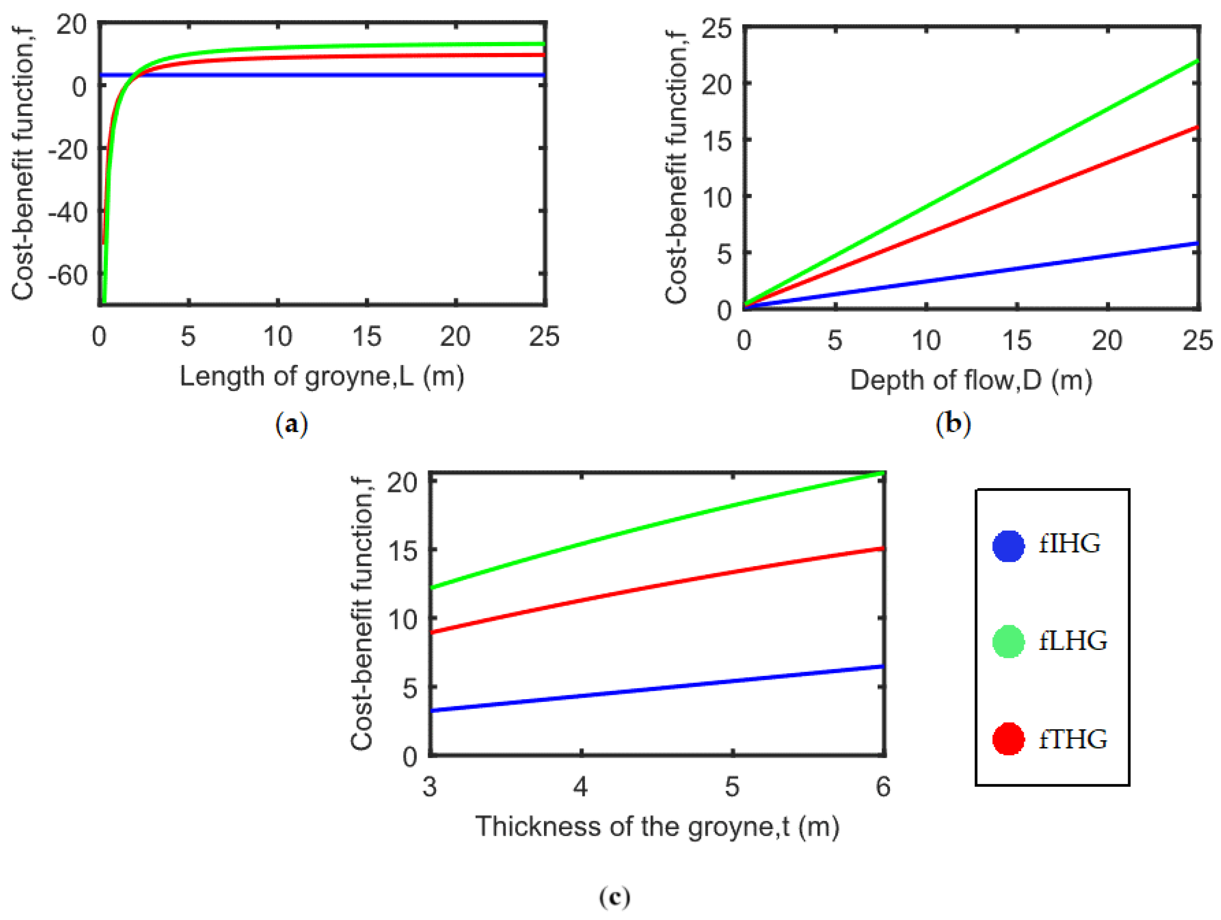
3.3. Cost–Benefit Analysis (CBA)
- i.
- Variable L with fixed D and t:
- ii.
- Variable D with fixed L and t:
- iii.
- Variable t with fixed L and D:
4. Conclusions
- i.
- Among the three groynes, LHG and THG show the most significant scour depths, with close values of 0.295 D and 0.29 D, respectively. IHG had a maximum scour depth of 0.21 D. The maximum scour depth for IHG is achieved near the tip of the groyne and can be attributed to the flow separation that occurs at that critical point. In the case of LHG, maximum scouring is achieved near the junction of both the faces of the groyne. However, for THG, the maximum scour depth occurs upstream of the groyne. This is due to the downflow upstream of the groyne when the flow hits the perpendicular face of the groyne and the HSV system that is the outcome of the downflow. This finding emphasizes the critical role of design and shape of the groyne on the flow characteristics and scour patterns.
- ii.
- The reduction in the normalized streamwise velocity and negative values is evident for the sections near groyne attached wall upstream of the groyne. This is attributed to the formation of HSV system. The peak of the normalized streamwise velocity is due to flow separation at the junction or tip.
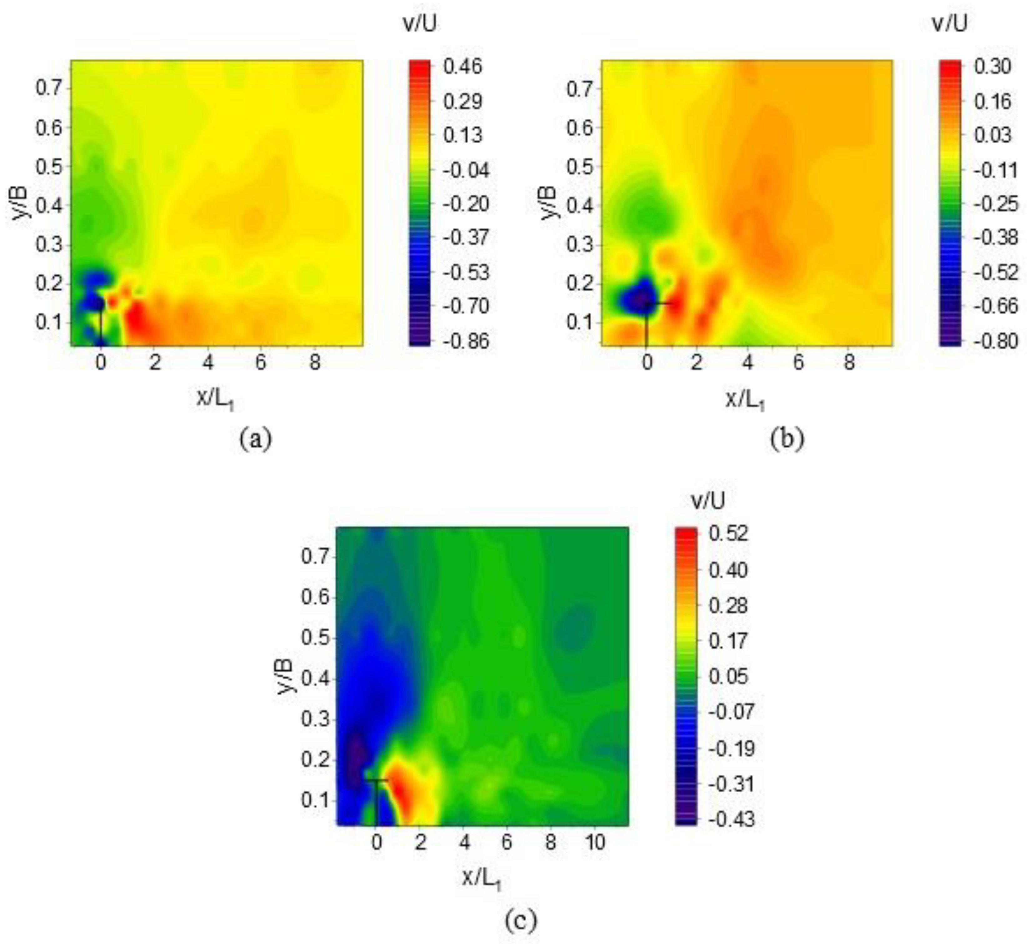
- iii.
- Shear layer formation, marked by an abrupt change in velocity direction, is observed along the line of flow divergence. The peak transverse velocity is observed near the groyne attached wall at the junction and within a small region downstream of the junction. This characteristic can be attributed to the occurrence of flow separation at the tip or junction of the groyne.
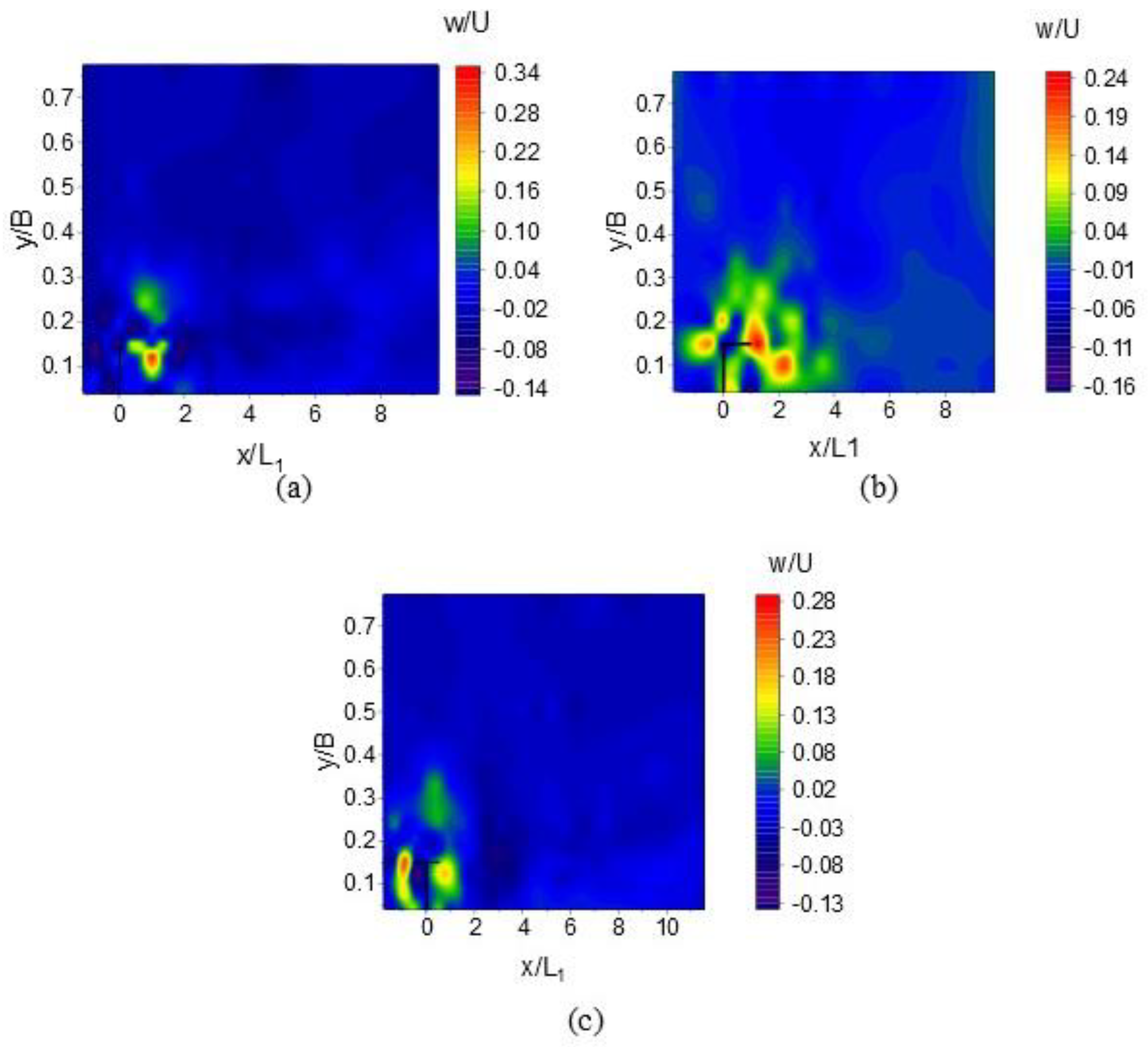
- iv.
- A strong upward flow is observed downstream of the groyne for all the groynes. Additionally, a strong upward flow is observed upstream of the groyne for THG and LHG which is absent for IHG. The increase in w/U upstream signifies downward flow upstream of the groyne, which is subsequently transferred downstream through the HSV.
Author Contributions
Funding
Institutional Review Board Statement
Informed Consent Statement
Data Availability Statement
Acknowledgments
Conflicts of Interest
Appendix A. Cost–Benefit Analysis for I Head Groynes (IHG), L Head Groynes (LHG), and T Head Groynes (THG)
- Flow depth, D;
- River width, B;
- Transverse length, L;
- Free board, FB;
- Thickness of groyne, t.
Appendix B. Cost Estimation for LHG
Appendix B.1. Cost Estimation
Appendix B.1.1. Cost of Concreting
Appendix B.1.2. Cost for Reinforcement
Appendix B.1.3. Excavation Cost
Appendix B.2. Total Cost for Construction of LHG
References
- Ouillon, S.; Dartus, D. Three-dimensional computation of flow around groyne. J. Hydraul. Eng. 2011, 18, 97–105. [Google Scholar] [CrossRef]
- Burele, S.A.; Gupta, I.D.; Singh, M.; Sharma, N.; Ahmad, Z. Experimental study on performance of spurs. ISH J. Hydraul. Eng. 2012, 18, 152–161. [Google Scholar] [CrossRef]
- Nayak, A.; Sharma, N.; Mazurek, K.A. Design Development and Field Application of RCC Jack Jetty and Trail Dykes for River Training. River Syst. Anal. Manag. 2017, 279–308. [Google Scholar]
- Blancett, J.; Asce, M.; Jarchow, P.; Asce, M. Kansas river bank stabilization and post-project conditions. In World Environmental and Water Resources Congress 2009: Great Rivers; ASCE: Reston, VA, USA, 2009; pp. 3400–3410. Available online: https://ascelibrary.org/doi/abs/10.1061/41036(342)343 (accessed on 1 May 2024).
- Yang, Q.-Y.; Wang, X.-Y.; Lu, W.-Z.; Wang, X.-K. Experimental Study on Characteristics of Separation Zone in Confluence Zones in Rivers. J. Hydrol. Eng. ASCE 2009, 14, 166–171. [Google Scholar]
- Zhang, H.; Nakagawa, H. Scour around Spur Dyke: Recent Advances and Future Researches. Annu. Disas. PREV. Res. Inst. Kyoto Univ. 2014, 51, 633–652. [Google Scholar]
- Zaghloul, N.A. Local scour around spur-dikes. J. Hydrol. 1983, 60, 123–140. [Google Scholar] [CrossRef]
- Kadota, A.; Suzuki, K. Local Scour and Development of Sand Wave around T-type and L-type Groynes. In Scour and Erosion; ASCE: Reston, VA, USA, 2010. [Google Scholar]
- Barbhuiya, A.K.; Dey, S. Vortex Flow Field in a Scour Hole around Abutments. Int. J. 2004, 18, 310–325. [Google Scholar]
- Kothyari, U.C.; Raju, K.G.R. Scour around spur dikes and bridge abutments. J. Hydraul. Res. 2010, 39, 367–374. [Google Scholar] [CrossRef]
- Dey, S.; Barbhuiya, A.K. Time Variation of Scour at Abutments. J. Hydraul. Eng. 2005, 131, 11–23. [Google Scholar] [CrossRef]
- Dey, S.; Barbhuiya, A.K. Velocity and turbulence in a scour hole at a vertical-wall abutment. Flow Meas. Instrum. 2006, 17, 13–21. [Google Scholar] [CrossRef]
- Kang, J.; Yeo, H.; Kim, C. Assessment of Habitats According to Groyne Types (Using Pale Chub). Engineering 2013, 5, 22–28. [Google Scholar] [CrossRef]
- Mall, M.; Priyanka; Hari Prasad, K.S.; Ojha, C.S.P. Development of a Framework for Cost—Benefit Analysis of I-Head and T-Head Groynes Based on Scour and Turbulent Flow Characteristics. Sustainibility 2023, 15, 15000. [Google Scholar] [CrossRef]
- Duan, J.G.; He, L.; Fu, X.; Wang, Q. Mean flow and turbulence around experimental spur dike. Adv. Water Resour. 2009, 32, 1717–1725. [Google Scholar] [CrossRef]
- Kumar, A.; Ojha, C.S.P. Near-bed turbulence around an unsubmerged L-head groyne. ISH J. Hydraul. Eng. 2019, 1–8. [Google Scholar] [CrossRef]
- Kadota, A.; Suzuki, K. Flow Visualization of Mean and Coherent Flow Structures around T-type and L-type Groynes. River Flow 2010, 2010, 203–210. [Google Scholar]
- Dehghani, A.A.; Azamathulla, H.; Najafi, S.A.H.; Ayyoubzadeh, S.A. Local scouring around L-head groynes. J. Hydrol. 2013, 504, 125–131. [Google Scholar] [CrossRef]
- Mortazavi Farsani, S. Numerical Simulation of the effect of simple and T-shaped dikes on turbulent flow field and sediment scour/deposition around diversion intakes. J. Mech. Contin. Math. Sci. 2019, 14, 197–215. [Google Scholar] [CrossRef]
- Vaghefi, M.; Ghodsian, M.; Ali, S.; Salehi, A. Experimental Study on Scour around a T-Shaped Spur Dike in a Channel Bend. J. Hydraul. Eng. 2012, 138, 471–474. [Google Scholar] [CrossRef]
- Raikar, R.V.; Dey, S. Clear-water scour at bridge piers in fine and medium gravel beds. Can. J. Civ. Eng. 2005, 32, 775–781. [Google Scholar] [CrossRef]
- Pandey, M.; Sharma, P.K.; Ahmad, Z.; Karna, N. Maximum scour depth around bridge pier in gravel bed streams. Nat. Hazards 2018, 91, 819–836. [Google Scholar] [CrossRef]
- Kuhnle, R.A.; Jia, Y.; Alonso, C. V Measured and Simulated Flow near a Submerged Spur Dike. J. Hydraul. Eng. 2008, 134, 916–924. [Google Scholar] [CrossRef]
- Yossef, M.F.M.; de Vriend, H.J. Flow Details near River Groynes: Experimental Investigation. J. Hydraul. Eng. 2011, 137, 504–516. [Google Scholar] [CrossRef]
- Mehraein, M.; Ghodsian, M. Experimental study on relation between scour and complex 3D ow field. Sci. Iran. 2017, 24, 2696–2711. [Google Scholar]
- Pokrajac, D.; Campbell, L.J.; Nikora, V.; Manes, C.; McEwan, I. Quadrant analysis of persistent spatial velocity perturbations over square-bar roughness. Exp. Fluids 2007, 42, 413–423. [Google Scholar] [CrossRef]
- Kirkgoz, M.S.; Ardiçlioğlu, M. Velocity profiles of developing and developed open channel flow. J. Hydraul. Eng. 1997, 123, 1099–1105. [Google Scholar] [CrossRef]
- Melville, B.W. Pier and Abutment Scour: Integrated Approach. J. Hydraul. Eng. 1997, 123, 125–136. [Google Scholar] [CrossRef]
- Goring, D.G.; Nikora, V.I. Despiking Acoustic Doppler Velocimeter Data. J. Hydraul. Eng. 2002, 128, 117–126. [Google Scholar] [CrossRef]
- Kwan, R.T.; Melville, B.W. Local scour and flow measurements at bridge abutments. J. Hydraul. Res. 1994, 32, 661–673. [Google Scholar] [CrossRef]
- Jeon, J.; Lee, J.Y.; Kang, S. Experimental Investigation of Three-Dimensional Flow Structure and Turbulent Flow Mechanisms Around a Nonsubmerged Spur Dike with a Low Length-to-Depth Ratio. Water Resour. Res. 2018, 54, 3530–3556. [Google Scholar] [CrossRef]


| Shape | D (m) | Fr | L1 (m) | L2 (m) | C.R. |
|---|---|---|---|---|---|
| IHG | 0.136 | 0.61 | 0.1125 | - | 15% |
| LHG | 0.136 | 0.61 | 0.1125 | 0.1125 | 15% |
| THG | 0.136 | 0.61 | 0.1125 | 0.1125 | 15% |
| x/L1 | (m/s) | Std. Dev. (m/s) | Skewness | Kurtosis | Std. Error (m/s) |
|---|---|---|---|---|---|
| 12.50 | 0.729797 | 0.081635 | 0.05941 | 2.708591 | 0.000868 |
| 8.00 | 0.751042 | 0.082159 | 0.15902 | 2.794846 | 0.000863 |
| 4.00 | 0.726126 | 0.081202 | 0.007192 | 2.876749 | 0.000875 |
| 0.00 | 0.791727 | 0.083517 | 0.21658 | 3.095242 | 0.000887 |
| 4.00 | 0.738749 | 0.083441 | 0.18728 | 2.881535 | 0.000856 |
| 8.00 | 0.837464 | 0.081221 | 0.17489 | 2.771532 | 0.001299 |
| 11.25 | 0.862593 | 0.080529 | 0.25855 | 3.312264 | 0.000826 |
| 15.00 | 0.879171 | 0.077864 | 0.21254 | 2.748936 | 0.000901 |
| 20.00 | 0.866055 | 0.084618 | 0.28543 | 2.758457 | 0.000878 |
| 25.00 | 0.83369 | 0.082747 | 0.1951 | 2.837325 | 0.001033 |
| 30.00 | 0.734824 | 0.096966 | 0.24464 | 2.791556 | 0.001046 |
| 35.00 | 0.642727 | 0.098407 | 0.02617 | 2.646666 | 0.000887 |
| 41.00 | 0.83348 | 0.085447 | 0.26433 | 2.773093 | 0.000909 |
| 47.00 | 0.739169 | 0.092991 | 0.0956 | 2.712638 | 0.000987 |
| 53.00 | 0.733704 | 0.093498 | 0.012802 | 2.782523 | 0.000993 |
| 59.00 | 0.810494 | 0.097884 | 0.27136 | 2.715227 | 0.001044 |
| 65.00 | 0.711532 | 0.097301 | 0.19889 | 2.651946 | 0.001806 |
| 75.00 | 0.651122 | 0.122696 | 0.16853 | 2.639037 | 0.00161 |
| 85.00 | 0.705159 | 0.100333 | 0.20404 | 2.752259 | 0.000863 |
| 95.00 | 0.67583 | 0.100405 | 0.24629 | 2.750138 | 0.001311 |
| 110.00 | 0.67236 | 0.099111 | 0.16994 | 2.690638 | 0.001311 |
Disclaimer/Publisher’s Note: The statements, opinions and data contained in all publications are solely those of the individual author(s) and contributor(s) and not of MDPI and/or the editor(s). MDPI and/or the editor(s) disclaim responsibility for any injury to people or property resulting from any ideas, methods, instructions or products referred to in the content. |
© 2024 by the authors. Licensee MDPI, Basel, Switzerland. This article is an open access article distributed under the terms and conditions of the Creative Commons Attribution (CC BY) license (https://creativecommons.org/licenses/by/4.0/).
Share and Cite
Priyanka; Mall, M.K.; Sharma, S.; Ojha, C.S.P.; Prasad, K.S.H. Investigating Flow around Submerged I, L and T Head Groynes in Gravel Bed. Sustainability 2024, 16, 7905. https://doi.org/10.3390/su16187905
Priyanka, Mall MK, Sharma S, Ojha CSP, Prasad KSH. Investigating Flow around Submerged I, L and T Head Groynes in Gravel Bed. Sustainability. 2024; 16(18):7905. https://doi.org/10.3390/su16187905
Chicago/Turabian StylePriyanka, Manish Kumar Mall, Shikhar Sharma, Chandra Shekhar Prasad Ojha, and K. S. Hari Prasad. 2024. "Investigating Flow around Submerged I, L and T Head Groynes in Gravel Bed" Sustainability 16, no. 18: 7905. https://doi.org/10.3390/su16187905
APA StylePriyanka, Mall, M. K., Sharma, S., Ojha, C. S. P., & Prasad, K. S. H. (2024). Investigating Flow around Submerged I, L and T Head Groynes in Gravel Bed. Sustainability, 16(18), 7905. https://doi.org/10.3390/su16187905