Abstract
This article presents an analysis of monthly precipitation totals based on data from the Global Precipitation Climatology Centre and monthly mean temperatures from the National Oceanic and Atmospheric Administration for 377 catchments located worldwide. The data sequences, spanning 110 years from 1901 to 2010, are analysed. These long-term precipitation and temperature sequences are used to assess the variability in climate characteristics, referred to here as polarisation. This article discusses the measures of polarisation used in the natural sciences. This study adopts two measures to evaluate the phenomenon of polarisation. The first measure is defined based on a stationary time series, calculated as the ratio of the amplitude of values to the standard deviation. The second measure is proposed as the difference in trends of these values. Based on the analysis of monthly precipitation data in the studied catchments, polarisation components are confirmed in 25% of the cases, while in the remaining 75%, they are not. For temperature data, polarisation is confirmed in 12.2% of the cases and not in the remaining 88.8%. The trend analysis employs Mann–Kendall tests at a 5% significance level. The Pettitt test is used to determine the point of trend change for precipitation and temperature data. This article underscores the complex relationship between climate polarisation and sustainable development, reaffirming that sustainable development cannot be pursued in isolation from the challenges posed by climate change. It emphasises the importance of integrating environmental, social, and economic strategies to adapt to extreme climatic events and mitigate their effects. This research is supported by detailed graphical analyses, with the results presented in tabular form.
1. Introduction
Analyses of historical observations of climate variables clearly indicate the anthropogenic causes of climate change [1,2,3]. Numerous studies at various spatial and temporal scales have thoroughly explored the impact of projected changes in the climate system on hydrology and water resources [3,4,5,6]. After air temperature, fresh water is proving to be the second most reactive environmental variable to climate change [7,8,9,10]. Despite the numerous existing studies and analyses of the temporal and spatial characteristics of precipitation and temperature, the timeliness of these studies is becoming increasingly appreciated [11,12,13,14,15,16,17,18], especially in the context of documenting the impact of human activities on regional climate factors [19,20,21]. Increasing computational capabilities and comprehensive analyses based on long measurement series [8,22,23] are attracting attention, especially in the context of the search for the justification of theses on the polarisation of extreme climatic events [24,25,26,27,28,29,30].
The increased interest in climatic factors such as precipitation and temperature [13,31,32] is also due to the consequences of floods and periods of hydrological drought [33]. Studies on the variability in precipitation and temperature over different periods [5,9,14,34,35,36] have made it possible to analyse statistical trends and assess the signal of these changes [32,37,38,39]. The results of these analyses provide information about the moments of trend change and the form of them. In the context of the importance of the variability in climatic factors, it is important to apply statistical techniques [4,40] that allow for the detection of changes and trends [2,38], in, among other sources, data relating to monthly precipitation totals and monthly average temperatures.
Climate change predicted by the IPCC (Intergovernmental Panel on Climate Change) occurs as a result of increases in greenhouse gas emissions, which are mainly caused by the industrialisation of the world, the burning of fossil fuels and changes in land use [3,10,41,42]. According to the Intergovernmental Panel on Climate Change [43], both natural forces and human activities contribute to changes in climate patterns, including increases in land and ocean surface temperatures, changes in spatial and temporal precipitation patterns, increases in the frequency of extreme events, rising sea levels, and increased El Niño [3,4,31,34]. It is clearly emphasised that human influence significantly outweighs the action of natural forces. The warming of the Earth is evident in data that show a 0.85 °C increase in global temperature from 1901 to 2012 [44]. To see changes in precipitation and temperature trends, anomalous values and statistical models are used to measure the timing of the trend change and its magnitude. The change in trends of various climate variables can be quantified using global atmospheric circulation models (GCMs) or, for example, using statistical models that identify the moment of change in the trend and its magnitude [8].
The polarisation of climatic elements is a phenomenon in which certain climatic elements or features tend to separate into two extreme or opposite categories [45,46]. This means that over time, certain climatic features become more clearly concentrated in the two opposite extremes, which can lead to increased variability and diversity in atmospheric conditions. Polarisation can manifest itself as a clear separation between extremes of temperature, precipitation, or other climatic parameters, with implications for long-term patterns and trends in the climate of an area. The property of bimodality emphasises the concentration of features in two opposite extremes [8,47,48,49]. The polarisation of precipitation events can be defined as a process in which the frequency and intensity of extreme precipitation events, such as rainstorms, hail, storms, or floods, increases. Simultaneously, the normal precipitation condition is becoming less frequent. In the case of temperature phenomena, polarisation can be defined as a process in which the frequency and intensity of extreme temperatures, such as heat waves or extreme cold, increases. Again, the normal state of temperatures is becoming increasingly rare. Both of these phenomena are part of a broader process of climate change that affects atmospheric circulation and processes, leading to increased weather variability and a greater risk of extreme weather. Polarisation can be interpreted as a change in the nature of the occurrence of extreme events, where extreme events, specifically extreme temperatures and precipitation, are becoming more frequent, while normal conditions are becoming less frequent.
It is important to note the strong connection between the variability in climatic phenomena, described here as polarisation, and sustainable development [50,51]. Changes in the frequency and intensity of extreme weather events, such as droughts, floods, or heatwaves, have a direct impact on the ability of societies and economies [52,53,54] to achieve sustainable development goals [55,56]. These phenomena not only test the resilience of infrastructure and socioeconomic systems but can also exacerbate existing inequalities, destabilise local and global markets, and accelerate environmental degradation [57,58].
In this study, the phenomenon of polarisation is analysed using selected river basins, identified as areas particularly vulnerable to extreme climatic events, both in terms of temperature and precipitation. Numerous studies indicate a significant impact of climate variability on river flow values, which are sensitive to changes in both precipitation and temperature. Researchers [35] have demonstrated the polarisation of climatic phenomena, identifying increasing trends primarily in the magnitude of floods in German river basins, attributing these changes to climate change. Additionally, seasonal analyses revealed that these changes were more pronounced in winter than in summer. Abrupt changes in both mean values and variance can be attributed to climatic factors (e.g., changes in climate regimes) as well as anthropogenic effects (e.g., construction of dams, changes in land use, vegetation cover, and shifts in measurement locations) [59,60]. The interpretation of statistical analyses must be conducted in the context of observed physical [3,7,61], social, and economic phenomena [3,14,19,62]. Therefore, predicting temporal trends in precipitation and temperature is crucial in social and urban planning [63].
The world’s rivers play a key role in linking the atmosphere, hydrosphere, and biosphere by transporting 40% of precipitation runoff and 95% of sediment to the oceans [64,65]. The shaping of river flow depends on many factors, such as precipitation, temperature, evaporation, soil conditions, landforms, and land use changes [66]. With the available long-term precipitation and temperature data, it is important to conduct long-term analyses of this data in order to understand the polarisation of climate phenomena and its potential consequences [67]. In addition, such analyses provide valuable information that can be used to develop decision-making tools for the purposes of effectively managing extreme events, such as droughts and floods, and to mitigate ecological damage in regions particularly vulnerable to these hazards [67].
When assessing climate polarisation, a process in which certain climatic features become concentrated in two opposing categories, there are strong links between precipitation and temperature [34,67,68]. An increase in global temperatures can lead to an increase in the amount of water vapour in the atmosphere. More water vapour in the atmosphere increases the potential for cloud formation and precipitation, especially in areas with higher temperatures where there is access to more thermal energy As a result, more water vapour may in turn increase precipitation, meaning that areas with higher temperatures may experience more precipitation. Conversely, lower temperatures can result in reduced precipitation. In extreme cases, such as prolonged droughts or floods, fluctuations in temperature and precipitation can have catastrophic consequences, including the failure of crops and damage to property [60,69].
Long-term data series make it possible to identify temperature and precipitation trends and help to determine whether a region is experiencing changes in polarity. Furthermore, the analysis of precipitation–temperature interactions provides a better link between important atmospheric phenomena, such as El Niño and La Niña cycles [70,71], which affect global climate patterns. An example of this is the fact that rising temperatures can affect the occurrence of intense precipitation, while reduced precipitation can contribute to extreme heat waves [60]. It is important to consider the amount of precipitation and temperature along with other climate phenomena as their interaction can affect the overall effect of climate polarisation [72]. The magnitudes and relationships between precipitation and temperature are crucial for assessing the polarisation of climate phenomena and its consequences for the environment, economy, and society. This knowledge is essential for implementing preventive measures to mitigate the negative effects of climate change.
The main focus of this study is the analysis of long-term precipitation and temperature data sequences with the aim of introducing the concept of climate extremes polarisation, using river basins as a case study. Section 1 provides a literature review and presents the background on extreme climate variability, which serves as the foundation for analysing polarisation phenomena. Section 2 explores the interactions between polarisation and sustainable development. Section 3 outlines the temporal and spatial scope of the data utilised in the analysis. Section 4 examines the phenomenon of polarisation in extreme climatic events, specifically in terms of precipitation and temperature, and discusses its significant consequences for ecosystems, economies, and infrastructure. Section 5 details the methodologies employed in constructing the polarisation measure and proposes the introduction of a static measure based on stationary time series as well as a dynamic measure based on trends. Section 6 and Section 7 present established statistical techniques for trend analysis and trend change point detection. Section 8 discusses and assesses the results of the analyses. Finally, Section 9 presents the conclusions.
2. Interactions between Polarisation and Sustainable Development
The polarisation of climatic phenomena, such as extreme precipitation and temperatures, presents additional challenges to the implementation of sustainable development [53,73], which strives for the harmonious coexistence of the economy, society, and the environment. Sustainable development is particularly vulnerable to disruptions resulting from global climate change, which can lead to the degradation of natural resources crucial for maintaining ecological balance. Such changes can also destabilise economies and cause social issues, such as migration driven by environmental changes [69].
In the context of natural resource conservation, the intensification of phenomena like droughts or floods can lead to the degradation of ecosystems and the depletion of water resources, threatening the ability of future generations to meet their needs. Variable climatic conditions also increase risks for agriculture, especially in urban areas where urban farming plays an increasingly important role in sustainable resource management [36,74]. Uneven distribution of rainfall and fluctuating temperatures can reduce agricultural productivity, impacting food security and economic stability in cities [75].
From the perspective of social justice, climate change can exacerbate existing inequalities, particularly among the poorest communities, which have limited capacity for adaptation [76]. Therefore, sustainable development must incorporate adaptive strategies that ensure equity and justice in resource access and protect the most vulnerable social groups. The long-term perspective of sustainable development requires integrating economic activities with ecological principles, taking into account dynamic climate changes [55]. Industry, transportation, and energy sectors must adapt their strategies, introducing innovations that minimise greenhouse gas emissions and support the development of a circular economy [52,54]. It is also necessary to strengthen policies and strategies at the global level that support sustainable development in the face of global climate challenges. Although the polarisation of climatic phenomena brings many challenges, it can also contribute to positive effects in the context of sustainable development [73].
Potential negative impacts:
- Degradation of natural resources: extreme phenomena such as droughts and floods can accelerate the degradation of natural resources, threatening ecological balance and future generations [77];
- Social inequality: the poorest communities, with limited capacity to adapt to climate change, are the most vulnerable to its negative effects, potentially deepening social inequalities [78];
- Impact on agriculture: variable and extreme climatic conditions can reduce agricultural productivity, affecting food security and economic stability, especially in urban areas [79,80];
- Challenges to infrastructure and industry: extreme weather events can disrupt the functioning of infrastructure and industry, leading to economic destabilisation [50];
- Risk to economic stability: economic losses caused by extreme events can lead to economic recessions, hindering the implementation of sustainable development strategies [50,79];
- Increased pressure on resources: growing pressure on limited natural resources can lead to conflicts over their availability, destabilising communities and economies [36,76].
Potential positive impacts:
- Acceleration of innovation and adaptation: extreme climatic conditions can stimulate the development of innovative technologies and adaptive strategies that minimise the negative impacts of climate change [51,60,81];
- Increased environmental awareness: climate polarisation can lead to greater social awareness of climate change, fostering more sustainable actions [82];
- Support for pro-environmental policies: support for sustainable development policies, such as reducing greenhouse gas emissions, protecting natural resources, and promoting the circular economy, is increasing [55,83];
- Increased efficiency and resilience of systems: communities and industries may strive for greater efficiency in resource use, reducing waste and supporting sustainable management [55];
- Growth of local and resilient Systems: local initiatives, such as urban agriculture, are gaining importance, increasing self-sufficiency and supporting sustainable development [53,84];
- Promotion of sustainable energy: climate change may accelerate the transition to renewable energy sources, which are more resilient to climate disruptions [51,54];
- Strengthening global cooperation: shared climate challenges may lead to closer international cooperation in support of sustainable development [85].
Sustainable development can play a key role in mitigating the effects of climate polarisation. However, it may also face challenges related to costs, delays in responses, and potential conflicts of interest. To effectively minimise negative impacts, an integrated approach is essential, combining sustainable development goals with adaptation to dynamically changing climatic conditions.
3. Preparation of Data for Analysis
This paper examines global trends in monthly precipitation totals and monthly mean temperatures from the area of 377 river basins distributed over all continents. Assuming 509.9 × 10⁶ square kilometres of land area on the earth, the analysis covers 12.76% of the total land area of the globe [86]. Table 1 shows the areas covered by the analysis. The regions in the text are identified by code , where (Table 1, Figure 1).

Table 1.
Areas covered by the analysis [86].
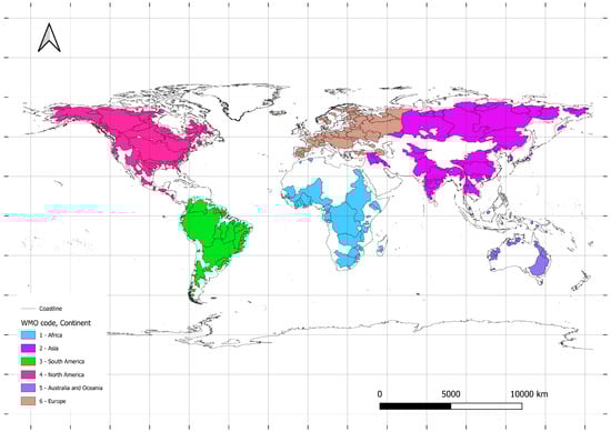
Figure 1.
Analysed catchments—WMO code and continent are marked.
Rainfall data from the GPCC and temperature data from NOAA for each month from 1901 to 2010, calculated based on grid data with a spatial resolution of 0.5° × 0.5° in latitude and longitude, were converted to catchment areas. This process generated a sequence of monthly data, which were then analysed in this study. Spatial data preparation involved the use of GIS interpolation techniques. The monthly precipitation/average temperature was calculated as a weighted average of the corresponding characteristic (precipitation/temperature) assigned to the grid cells covering the catchment area, with the weight proportional to the area of the grid cell [86]. The interpolation program was written in MATLAB (version R2021a) (The MathWorks, Inc.: Natick, MA, USA) by the author.
The area of one of the smallest catchments in this study, Skjern A (Europe, Denmark) is, according to calculations, 1090 km2. An area of 0.5° × 0.5° at the latitude of Denmark covers an area of 3100 km2. The location of this catchment area, for calculations of precipitation or temperature, requires the consideration of five neighbouring areas of 0.5° × 0.5°. With even such a small catchment area, precipitation and temperature characteristics are averaged. The calculated values of the sequences were subjected to a simple statistical analysis, determining the basic statistics: the minimum and maximum value, the mean, and the standard deviation of the sample. The data were analysed in monthly as well as calendar year cross-sections. Analyses of temperature data covered the years 1901 to 2010.
4. The Polarisation of Precipitation and Temperature Phenomena
The assessment of temporal variability and extreme events in air temperature and precipitation typically involves analysing a set of indicators that define these conditions. The concept of an extreme event assumes the existence of a normal state [39]. In this context, polarisation can be understood as a shift in the occurrence of extremes, with extreme temperatures and precipitation becoming more frequent, while the normal state becomes less common [87]. This polarisation can result from various factors, including human activity and climate change, which influence precipitation cycles, the intensity of extreme events, and temperature patterns. Consequently, polarisation represents the evolution of climatic features, leading to an increase in the frequency of extreme events and a destabilisation of the typical climate state. This shift can have significant consequences for ecosystems, the economy, and human quality of life.
The analysis of precipitation and temperature polarisation is crucial due to their central role in global energy and water cycles, as well as their impact on climate change. These variables are particularly important for managing freshwater resources and mitigating the risks of floods and droughts. Increasing evidence suggests that human activities are accelerating climate change, leading to shorter periods of intense precipitation and longer dry spells marked by high temperatures and low precipitation [87]. The growing evidence of polarisation in extreme events, such as floods and droughts, underscores the uneven and intense impact of human activity on the climate.
This article examines long-term sequences of precipitation and temperature to evaluate the polarisation of climate phenomena. In climate science, “polarisation” describes the process by which certain areas of the planet experience more extreme temperature and/or precipitation conditions. This can lead to significant local environmental changes, including shifts in the distribution of plant and animal species, alterations in weather patterns, and changes in sea levels [88]. Long-term sequences of precipitation and temperature are critical for studying climate polarisation, providing detailed records that help identify trends and patterns. By analysing these sequences, researchers can pinpoint areas where the climate is becoming increasingly polarised and monitor changes over time. The use of these sequences offers a high degree of accuracy and precision, thanks to advanced measurement techniques and rigorous quality control measures [27,89,90].
The impact of polarisation extends across various aspects of life on Earth, affecting ecosystems, the economy, and infrastructure, as well as altering the size and location of water resources. In ecosystems, extreme temperature and precipitation changes influence biodiversity and ecosystem functioning, potentially leading to shifts in the distribution of plant and animal species, with negative consequences for entire ecosystems [88]. In agriculture, polarisation can reduce available water resources, impacting crop yields and food production [17,36,91,92]. For infrastructure, polarisation can lead to damage or destruction of roads, bridges, buildings, and water management systems. Given the complex and dynamic nature of the climate, polarisation is variable and difficult to predict, making it challenging to foresee its specific consequences in any given region [93,94].
The interaction between polarisation and other climate phenomena can trigger events such as hurricanes, tornadoes, or droughts, where one phenomenon may amplify or weaken another, complicating the understanding of climate change. Anthropogenic factors, particularly greenhouse gas emissions, play a significant role in driving the polarisation of climate factors [17,67,92].
The summary of causes and effects of polarisation presented below shows the complex nature of this phenomenon, where the clear separation of the two extreme categories leads to a variety of consequences, producing effects that dominate on many levels.
Causes of polarisation of precipitation phenomena:
- Changes in atmospheric circulation: fluctuations in atmospheric circulation, such as changes in belt and monsoon patterns, can concentrate precipitation in certain regions, while other areas experience precipitation deficits [95];
- El Niño and La Niña phenomena: these can lead to abrupt changes in ocean surface temperature, which affects rainfall patterns; areas that are normally wet can experience drought during El Niño, and dry areas can become flooded during La Niña [46];
- Topographical changes: high mountain ranges can affect the movement of air masses and cloud formation, leading to more rainfall on one side of the mountain and droughts on the other [46];
- Urbanisation and land use changes: urban growth and land use changes can alter the microclimate and affect the distribution of precipitation in an area [46].
Causes of polarised temperature phenomena:
- Melting of glaciers and reduction in ice cover: these can affect surface albedo, which can lead to faster warming in polar areas and cooling in oceanic areas [49,96];
- Changes in atmospheric circulation: may bring higher temperatures to tropical areas, while areas under the influence of lows may experience cooling [95];
- Changes in greenhouse gases: increases in greenhouse gas concentrations can lead to an overall warming of the climate, but some areas may experience faster temperature increases than others [72];
- Impact of urban areas: cities create so-called “heat islands” where concrete and asphalt absorb and retain heat, which can lead to significant heating of urban areas [97].
Effects of polarised precipitation events:
- Increased weather variability: polarisation of precipitation can lead to abrupt and unpredictable changes in weather patterns, which can make planning for agricultural and infrastructure activities difficult [36];
- Risk of natural disasters: extremes of rainfall can increase the risk of natural disasters, such as floods in areas of increased rainfall or droughts in areas of decreased rainfall [60];
- Impact on water availability: precipitation polarisation can lead to reduced water availability in drought-affected areas and increased risk of soil erosion during periods of intense rainfall [98];
- Impact on ecosystems: extreme precipitation conditions can affect ecosystem structures and services, with potential implications for biodiversity and ecosystem products [84].
Effects of polarised temperature phenomena:
- Human health risks: temperature extremes, both heat and cold, can pose a risk to human health, leading to heat- or cold-related diseases [60];
- Effects on agriculture and food production: extreme temperatures can affect plant growth processes, leading to reduced yields and loss of quality in agricultural products [80];
- Changes in species distribution: extreme temperatures can affect the distribution areas of different animal and plant species, which can disrupt the balance of ecosystems [99];
- Changes in water levels: glacial melting and ocean warming associated with temperature polarisation can lead to rising sea and ocean levels [100].
Interaction effects of precipitation and temperature polarisation:
- Increased risk of natural disasters: the combination of extreme rainfall and temperatures can amplify the risk of floods, landslides, and other natural disasters [76];
- Impact on agri-food production: extreme precipitation and temperatures can negatively affect food production, which can lead to food security problems [60];
- Changes in the landscape: the interaction of extreme rainfall and temperatures can lead to changes in the landscape, such as soil erosion and degradation of natural areas [60].
5. The Concept of Polarisation Measure
The concept of measuring climate polarisation is based on measuring the degree of diversity and variability in climate elements in a given area. This measure is used to determine the level of polarisation of climate elements in the region of interest. Polarisation refers to the extremes of parameters such as temperature, precipitation, humidity, etc., occurring in a specific area. A high level of polarisation indicates significant differences between maximum and minimum values, which can lead to an increased risk of extreme weather events. The measure of polarisation can be determined from various climatic parameters, such as temperature, precipitation, humidity, and atmospheric pressure. This can be calculated on different spatial and temporal scales, for example, for the entire country over the course of a year, for a specific region over the course of a month, or for individual weather stations over the course of a day. Depending on the purpose of the study and the availability of data, the measure of polarisation can be determined for different combinations of parameters. It is worth noting that a high level of polarisation does not necessarily mean unfavourable climatic conditions. For example, some regions have significant temperature differences between summer and winter, which can have a positive impact on seasonal tourism. However, in other cases, high polarisation can lead to serious problems, such as droughts, floods, or storms. Therefore, a measure of polarisation can be useful in identifying areas that require special attention when planning climate change adaptation activities.
Different approaches are possible for constructing measures of polarisation in climate phenomena, depending on the type and scale of the data under analysis. One of the basic methods is to use probabilistic techniques based on classical theories of one- or multi-dimensional random variables with distributions built using Copula functions [63,101,102]. Other, simpler methods are based on statistical characteristics [4,10,40,47]. A simple concept is to construct indicators measuring the degree of extremity that a phenomenon can take, for example, by measuring the dispersion relative to the long-term average. An example of such an indicator is the coefficient of variation. Another way to create a polarisation indicator is to define it as the degree of extremity compared to the mean value relative to the variability measured by the dispersion measure [12,103,104]. Such indicators can be based on classical measures, such as variance, standard deviation, mean deviation, and the coefficient of variation, or on positional measures, such as range, quartile deviation, and the coefficient of variation [47].
Further methods of building indicators are based on the idea of unevenness [85,105], which can also be a measure of polarisation. One such indicator is kurtosis [106], which is influenced by the intensity of extreme values, so it measures what is happening in the “tails” of the distribution. Other types of indicators are measures that have their genesis in economics and econometrics. One such example is the Gini index, also called the Gini coefficient [78,104,107,108,109], built using the Lorentz curve, which describes the degree of concentration of a one-dimensional distribution of a random variable with non-negative values [108]. The Gini index ranges from a minimum value of zero, when all values are equal, to a theoretical maximum of one in an infinite population in which every element except one has a magnitude of zero. In the context of climate change, the Gini index can be used to measure inequality in exposure to the effects of climate change, such as droughts, floods, or sea level rises [72]. Higher values of the Gini index indicate greater inequality in the occurrence of these phenomena. Several other examples of measures can be cited, including the following:
- The concentration ratio [110] determines the degree of concentration of values at one end of the distribution and is similar to the Gini coefficient. However, it should be noted that the Gini coefficient may be less useful in analysing asymmetric distributions, which means that other indicators such as the concentration ratio or Lorenz curve should be considered in such cases.
- The GMD (Gini mean difference) index [111] is an inequality measure used in statistical and econometric analysis to measure polarisation or inequality in a sample distribution. Unlike the Gini coefficient, which measures unevenness, the GMD index enables the analysis of unevenness in the distribution of any variable, such as income, age, weight, height, precipitation, or temperature. The GMD index ranges from zero to one, where zero indicates complete evenness in the distribution and one indicates the concentration of all values in one class. The higher the GMD index value, the greater the unevenness in the variable distribution.
- The Theil index [78,112] is a measure of inequality in the distribution of quantitative variables, based on the idea of information entropy, taking into account differences between groups of values in the distribution, similar to the Gini coefficient, but with a greater emphasis on extreme values.
- The Lorenz indicator [105,108] is an inequality indicator in a distribution, which is based on the Lorenz curve. It is often used to measure income inequality but can also be used to measure inequality in other quantitative variables, including climate change studies. Higher values of the Lorenz curve indicate greater inequality in the occurrence of climate change effects such as droughts, floods, or sea level rises, meaning that some regions or social groups are more vulnerable to the effects of climate change than others.
- The Atkinson index [104] is a measure of inequality in the distribution of quantitative variables, which is based on the idea of absolute deviations. It takes into account the differences between groups of values in the distribution; it is similar to the Gini index, but focuses more on average values than extreme values.
- Range relates to values calculated as max–min usually referring to the difference between the maximum and minimum values of a given variable in a specific period of time. In the case of assessing the polarisation of precipitation and temperature, max–min can be used as a measure of the amplitude of these variables in a given period.
In this study, two measures are adopted to evaluate the phenomenon of polarisation, the first is built based on a stationary time series, the second is based on calculated trends. The first measure is defined as follows:
where for precipitation:
, [mm]—the maximum value of monthly precipitation totals over the 110-year period;
, [mm]—the minimum value of monthly precipitation totals over the 110-year period;
, [mm]—the standard deviation of monthly precipitation over the 110-year period;
for temperature:
, [°C]—the maximum value of monthly average temperature over the 110-year period;
, [°C]—the minimum value of monthly average temperature over the 110-year period;
, [°C]—the standard deviation of monthly average temperature over the 110-year period;
, []—a measure for assessing the phenomenon of polarisation, based on a stationary time series.
The second measure is defined as follows:
where for precipitation:
, [mm/year]—this is the trend of the amplitude of changes over a 110-year period, calculated based on annual extreme values;
, [mm/year]—this is the trend of the standard deviation over a 110-year period, calculated based on annual extreme values;
for temperature:
, [°C/year]—this is the trend of the amplitude of changes over a 110-year period, calculated based on annual extreme values;
, [°C/year]—this is the trend of the annual standard deviation over a 110-year period.
The above measure can be interpreted as the ratio of the trend in variability in the amplitude to the trend in variability in the standard deviation. The trend in variability in the amplitude refers to the direction and speed of changes in the maximum and minimum values of a given variable over time, while the trend in variability in the standard deviation refers to the direction and speed of changes in the variability in the values of a given variable around their mean over time.
The amplitude of change values can be useful in identifying extreme climate conditions, such as periods of drought or heat waves, as well as periods of intense precipitation or extremely low temperatures. However, max–min as a single measure may be limited in its usefulness because it does not take into account other factors such as the length and intensity of the period, as well as other variables that affect weather conditions. Due to the fact that it ignores all data except for two extreme values, it does not provide information about the diversity of individual feature values in the population. Therefore, along with max–min values, other measures such as mean values, standard deviations, or cumulative indices are typically used to obtain a more comprehensive and diverse view of climate variability. For example, max–min values can be calculated for individual months, seasons or years, and then compared with mean values, standard deviations, or other measures to better describe climate variability over time and space.
The adopted measure, which is the ratio of the max–min values to the standard deviation , can be used as a measure to evaluate the polarisation of precipitation and temperature. The values refer to the amplitude of changes in a given variable over a period of time, while the standard deviation σ refers to the degree of variability in these values around their mean. By applying this measure, we can see how large the amplitude of changes is in relation to the variability around the mean. Values of this measure greater than 1 suggest that the amplitude of changes is greater than the variability around the mean. If the variability is relatively low compared to the amplitude, it may indicate the occurrence of periods of extreme climatic conditions, such as periods of drought or heatwaves, as well as periods of intense rainfall or extremely low temperature. However, the use of a single measure may be limited because it does not take into account other factors affecting climate variability. Therefore, it is worth using it together with other measures that show the character of climate variability. Note that the values of this measure for precipitation and temperature will always take a non-negative value.
The second form of adopted measures could be dynamic indicators showing the variability in the indicator over a longer period of time. The simplest indicators are based on the idea of a trend coefficient. Trend is a long-term feature referring to the general direction of changes over time in the value of a variable. Trend can indicate an increase, decrease, or stabilisation of the variable over time. In time series analysis, the trend coefficient is one of the basic elements that help to forecast future values of the variable. The trend can be analysed for different time scales, from short-term cycles to long-term trends [2]. Trend analysis is applied in many fields, such as economics, finance, meteorology, earth sciences, medicine, sociology, and marketing. In scientific research, trend analysis is often used to study changes in long-term time series, such as climate change, demographic changes, or evolution of species.
The values of this measure according to the direction of change and the relationship of the components of the measure are interpreted in Table 2. The compatible signs of the components and were assumed. This assumption is based on the experience obtained in this analysis. In the calculations carried out for all catchments in both precipitation and temperature data at a significance level of 5%, if exists, then also exists and vice versa. Both components are highly correlated and have the same signs.
Table 2.
Trends in the components of measure P2 and their relationships and relevance to climate change.
6. Detecting a Change Point in the Trend
Various methods can be applied to determine change points in a time series [8,113,114,115,116]. In this analysis, the non-parametric Pettitt change point test (PCPT) [117] was used to detect the occurrence of changes. The Pettitt test (PCPT) is a non-parametric test for detecting sudden changes in a time sequence. It is used to detect the turning point where a sudden change, known as a “jump”, occurs in the time series. The Pettitt test (PCPT) involves comparing the sum of ranks of two subsets of data, which are divided by a threshold value, to determine whether there is a statistically significant change in the time sequence.
This test can be applied to analyse data with any distribution, and the test result is not dependent on the data having a normal distribution. The result of the Pettitt test (PCPT) is a test statistic value, which is compared with the critical value for the level of significance to determine whether the null hypothesis of no sudden changes in the time sequence can be rejected. The rank is given after sorting and is dependent on the variable that gives the order of the records in the set.
The PCPT has been widely used to detect changes in observed climatic and hydrological time series [8,16,98,118]. The Pettitt test is also applicable to investigate an unknown change point by considering a sequence of random variables , which have a change point at . As a result has a common distribution , but have a different distribution , where . The null hypothesis, : no change (but ), is tested against the alternative hypothesis, : change (lub ), using the non-parametric statistic , where the following applies:
for the downward shift and or the upward shift [116]. The confidence level associated with lub is approximately determined as follows:
when is smaller than the specified confidence level (for example, in this study, 0.95 was adopted), the null hypothesis is rejected. The approximate probability of significance for the change point is defined as follows:
It is obvious that in the case of a significant change point, the series is segmented at the change point into two sub-time series.
The main aim of this study is to investigate the existence of change points in the time series of monthly sum precipitation and monthly average temperature characteristics. For time series showing a significant change point, the trend test is applied to partial series, and if the change point is not significant, the trend test is applied to the entire time series [8].
The Pettitt change point test (PCPT) is highly valuable in the context of sustainable development, as it enables the identification of tipping points where significant shifts in precipitation or temperature have occurred. A sudden decrease or increase in precipitation may indicate the need to adjust water resource management systems to adapt to new climatic conditions. The results of this test can highlight the urgency for swift responses to evolving climate patterns. Detecting a change point can signal the immediate need for adaptive measures to minimise potential negative impacts of climate change, such as floods, droughts, or shifts in water availability.
7. Trend Test
To examine the trend in a given time series, the Mann–Kendall test (MKT) can be applied. Originally, this test was used by Mann [119], and later, Kendall derived the distribution of the test statistic in 1975 [116]. This test is independent of the type of distribution, and we do not need to adopt any specific form of the data distribution function [120]. This test was widely recommended by the World Meteorological Organization for public applications and has been used in many scientific studies to assess trends in water resource data [2,8,116]. Therefore, the MKT has been recognised as an excellent tool for trend detection by other scholars in similar applications. It should also be noted that the MKT considers only the relative values of all elements in the series . for analysis. The test statistic for the MKT is given by the following:
where are the consecutive values of the data and n is the number of elements in the data. Under the null hypothesis of no trend, and assuming that the data are independent and identically distributed with a zero mean and a variance denoted by , which is calculated as (—the repeated values in the analysed sequence):
To test a hypothesis, the standard normal distribution is used, denoted as the test statistic , which is defined as follows for the trend test:
In the two-sided test for trend, the null hypothesis is represented as follows: : there is no trend in the dataset, which will be rejected if the calculated statistic is greater than the critical value of this statistic obtained from the standard normal distribution table corresponding to the previously established level of significance. A positive value of indicates an increasing trend, and a negative value indicates a decreasing trend.
The magnitude of the trend is estimated using a non-parametric slope estimator based on the median proposed by Sen [121] and extended by Hirsch [122]. The slope estimator is given as follows:
where , and is treated as the median of all possible pairs of combinations for the entire dataset.
The Mann–Kendall Test (MKT) allows for the identification of long-term trends in precipitation and temperature, which is crucial for understanding whether persistent climate changes are occurring that could impact sustainable development. The results of the MKT can inform decisions related to climate and environmental policies. If the test reveals significant changes in the climate, it may necessitate the implementation of appropriate measures, such as adjustments to water resource management regulations, to ensure ecological and socioeconomic stability.
8. Results and Discussion
In the present study, the following properties of long-term sequences of monthly precipitation totals and monthly mean temperatures were investigated for 377 catchments across six WMO regions. The scope of the research and calculations included the following:
- Determining the values of long-term monthly series over a 110-year period;
- Calculating statistics related to the average values for each calendar month, including the minimum, maximum, mean, and standard deviation;
- Determining trend values using the Mann–Kendall test (MKT) to evaluate trends;
- Examining whether the long-term series exhibited change points using the Pettitt test (PCPT);
- Investigating whether the sub-series (after the identified change point up to 2010) showed a significant trend and how this trend differed from the long-term series in cases where change points were identified.
Of all the catchments analysed in terms of monthly precipitation totals, only one—the Lagarfljót River catchment in Iceland (Europe)—satisfied all four tests (MKT for RANGE, MKT for STD, PCPT for trend change, and MKT for new trend) simultaneously. This means that, at the 5% significance level, the P2 measure trend was identified for this catchment, the year of the trend change was determined, and a new trend was additionally recognised. The RANGE trend not only changed in value but also in direction, shifting from negative to positive, with a change from (−0.136) to (0.310) in 1953. Similarly, the STD trend changed from (−0.533) to (0.889) in the same year.
In the case of the Lagarfljót catchment, both the values and directions of the RANGE and STD trends shifted. The change in the RANGE trend from negative to positive in 1953 indicates an increase in the maximum monthly precipitation values in the study area. Additionally, the change in the STD trend reflects a shift in the variability of this phenomenon. The primary driver behind these changes appears to be the economic and demographic development in the region. In 1947, the town of Egilsstaðir was founded along the banks of the Lagarfljót River, becoming the largest town in eastern Iceland and its main service, transport, and administrative centre. By the 1950s, Iceland experienced a significant increase in the use of oil for heating, contributing to increased CO2 emissions, rising temperatures, and potentially influencing changes in precipitation patterns [123].
However, this remains a hypothesis, as it is challenging to directly link local emissions to specific climate changes without more advanced analyses, such as climate modelling. Even though global emissions were lower at that time, asserting that local CO2 emissions alone caused synoptic climate changes in the region would require further evidence. Only detailed simulations and analyses could confirm whether local emission changes had a measurable impact on precipitation patterns, particularly within a global context.
Based on the analysis of monthly precipitation data from the 377 catchments, it was found that for 93 catchments (25% of the total), the trends in polarisation coefficients (RANGE and STD) for monthly precipitation totals were statistically significant at the 5% level. In contrast, no significant trends were identified in the remaining 75% of the catchments.
Analysis of the P1 polarisation coefficient values (Figure 2, Table 3) across the ten largest catchments, with areas ranging from 1,705,383 to 4,640,300 km², reveals notable variations in precipitation patterns. The coefficient of variation within these catchments ranges from 0.29 to 1.0, indicating a significant disparity in the consistency of monthly precipitation totals. Meanwhile, the P1 measure, spans from 4.25 in the Yenisei catchment (Russian Fed., Asia) to 5.54 in the Mississippi River catchment (United States, North America). Across all analysed catchments, the P1 measure exhibits an even broader range, from 3.81 in the Ganges catchment (India, Asia) to 12.78 in the Copper River catchment (United States, North America). These findings highlight substantial differences in precipitation variability and extremes between different regions. Higher P1 values suggest that some catchments, particularly the Copper River, experience more pronounced fluctuations in monthly precipitation, which could indicate greater susceptibility to extreme weather events such as floods or droughts. Conversely, lower P1 values, like those observed in the Ganges, may indicate more stable precipitation patterns, although this does not necessarily imply a lower risk of extreme events. The wide range of P1 values across these large catchments underscores the importance of regional climate characteristics and their impact on hydrological extremes.

Figure 2.
Polarisation measure for monthly precipitation totals of the period 1901 to 2010.
Table 3.
P1 measure values for precipitation in the ten largest catchments.
The values (Figure 3, Table 4) of the P2 polarisation component trends are shown at the 5% significance level. The following values were obtained from the next ten largest catchments ranging from 244,000 to 2,900,000 km2: the P2 measure takes values from −0.895 (Brahmaputra, Bangladesh, Asia) to 0.444 (Uruguay, Uruguay, South America). The range of values of this measure for all analysed catchments meeting the 5% significance criterion takes values from −0.966 (Purari, Papua New Guinea, Australia and Oceania) to 0.945 (Han-Gang (Han River), Korea, Rep., Asia).
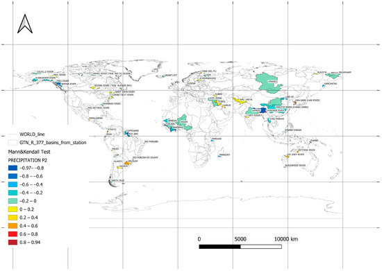
Figure 3.
Watersheds in which significant polarisation trends were identified for monthly precipitation sums during the period from 1901 to 2010 at a significance level of 5%.
Table 4.
Trend values of P2 polarisation components for precipitation at 5% significance level in the ten largest catchments.
Figure 4 shows the spatial location of the analysed catchments, where significant trend change-points in the polarisation coefficients of monthly precipitation were recognised at the 5% significance level (Table 4). For the catchments of the rivers of Africa, the years of changes in rainfall trends mainly occur in the late nineteen-sixties to the nineteen-seventies. Changes in trends can be linked to processes of decolonisation, independence, and economic development in the area. The apogee of this process occurred between 1960 and 1968, and 1960 is referred to as the “Year of African Independence” [124]. For the catchments of the rivers of Asia, the years of changes in rainfall trends mainly occur in the range of the nineteen-fifties to the nineteen-sixties in the area of Russia, the nineteen-forties to the nineteen-sixties in the area of China, and from the nineteen-thirties to the nineteen-seventies in the area of India. The 1950s in Russia saw intensive economic development, industrialisation, and intensive agricultural development [125]. The year 1949 was the beginning of land reform and nationalisation of the main economic sectors in China. The 1970s was the Cultural Revolution, where economic development collapsed [126]. For the catchment areas of South American rivers, years of changes in precipitation trends mainly occur in the period from the nineteen-forties to the nineteen-seventies. The 1960s and 1970s were a watershed period in the economic development of Latin American countries [127]. In the area of North America, this period is from the nineteen-forties to the nineteen-sixties on the west coast and through the nineteen-sixties for the east coast. This is a period of industrial and demographic boom [126]. For the catchments of the rivers of the Australia–Oceania area, trend changes have been shown in the years from the nineteen-fifties to the nineteen-seventies. This is a period of intense industrial development and demographic growth, as well as the decolonisation of Oceania and its economic development [126].
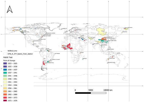
Figure 4.
Watersheds in which change-points in the trend of factors related to precipitation polarisation for monthly precipitation sums during the period from 1901 to 2010 were identified at a significance level of 5%.
The reasons for the change in precipitation trends in the analysed catchments may be related to a variety of climatic, geographical, and anthropogenic factors. Potential causes of changes in rainfall trends by region are outlined below:
- Africa: changes in atmospheric circulation, including fluctuations in the rainfall belt and belt patterns, El Niño and La Niña phenomena, deforestation, overgrazing of animals and changes in land use, and land degradation [31,46];
- Asia: diversity of topography can affect air mass movements and precipitation formation; changes in atmospheric circulation such as monsoons; increasing urbanisation and infrastructure development can create the so-called “heat island effect”, which affects the microclimate; air pollution including particulate matter, which affects condensation and cloud formation [31,128];
- South America: atmospheric circulation fluctuations, including those associated with El Niño and La Niña; topography of the region, including the Andes; deforestation; conversion of land for agriculture and urbanisation [46];
- North America: changes in atmospheric circulation such as the North Atlantic Oscillation, deforestation, urbanisation and land use change, and greenhouse gas emissions [31,44];
- Australia and Oceania: El Niño–La Niña cycle, changes in ocean circulation, variation in ocean surface temperature and atmospheric pressure between western and eastern areas of the Indian Ocean, deforestation, change in water use and air pollution, intensive agriculture, and overexploitation of water resources [31,46].
Based on the analysis of the data of monthly average temperatures in the analysed catchments, it should be noted that for 46/377 catchments, i.e., in 12.2% of the analysed catchments, the trends of polarisation coefficients in the range of temperatures were proven at the significance level of 5%, and in the remaining 88.8, they were not confirmed.
The analysis of the temperature polarisation index (Figure 5, Table 5) across ninety-three catchments reveals significant variability in the P1 index, ranging from a high of 10.43 for the Sepik River catchment (Australia and Oceania, Papua New Guinea) to a low of 3.26 for the Indigirka River catchment (Asia, Russian Fed.). These results indicate that the Sepik River catchment experiences the most pronounced temperature fluctuations among the studied regions, which could suggest a greater vulnerability to extreme temperature events. On the other hand, the lower P1 value for the Indigirka River catchment suggests more stable temperature conditions, although this does not necessarily correlate with a lower risk of temperature extremes. The observed variation in the P1 index among the catchments underscores the diverse nature of temperature polarisation across different geographic regions. For instance, the Sepik River, with the highest P1 value, may be more susceptible to dramatic temperature swings, which could have significant implications for local ecosystems and human activities. In contrast, catchments like the Indigirka River, with lower P1 values, may experience more consistent temperature patterns, though they are not immune to extreme events. The data also show some interesting patterns among the larger catchments, such as the Amazonas in Brazil and the Congo in Africa, which exhibit relatively high P1 values, suggesting notable temperature variability. Meanwhile, catchments like the Mississippi River in the United States and the Yangtze River in China show lower P1 values, indicating less temperature variability.
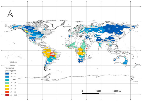
Figure 5.
Polarisation measure P1 for monthly temperature totals of the period 1901 to 2010.
Table 5.
P1 measure values for temperature in the ten largest catchments.
The values (Figure 6, Table 6) of the P2 polarisation component trends are shown at the 5% significance level. The following values were obtained from the next ten largest catchments ranging from 120,764 to 1,730,000 km2: the P2 measure takes values from −0.018 (Amur, Russian Fed., Asia) to 0.005 (Sao Francisco, Brazil, South America). The range of values of this measure for all analysed catchments meeting the 5% significance criterion takes values from −0.018 (Amur, Russian Fed., Asia) to 0.022 (Arnaud, Canada, North America).
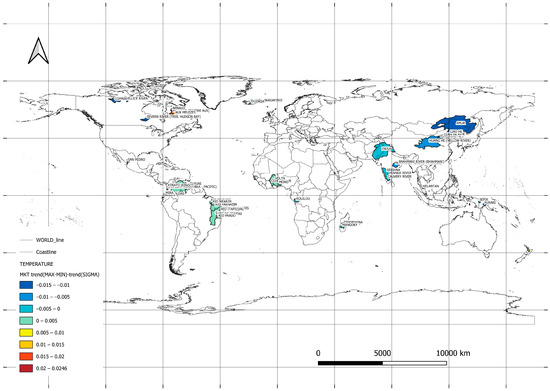
Figure 6.
Watersheds in which significant polarisation trends were identified for monthly mean temperatures during the period from 1901 to 2010 at a significance level of 5%.
Table 6.
Trend values of P2 polarisation components for the next ten largest catchments at 5% significance level for temperature.
Figure 7 shows the spatial location of the analysed catchments, where significant trend change-points in the polarisation coefficients of monthly mean temperatures were recognised at the 5% significance level (Table 6). For the catchments of African rivers, the years of changes in precipitation trends mainly occur in the nineteen-sixties to nineteen-eighties.

Figure 7.
Watersheds in which change points in the trend of factors related to temperature polarisation for monthly mean temperatures during the period from 1901 to 2010 were identified at a significance level of 5%.
For the catchments of Asian rivers, the years of changes in precipitation trends mainly occur in the nineteen-forties to the nineteen-sixties. For the catchments of South American rivers, years of changes in rainfall trends mainly occur in the nineteen-thirties to the nineteen-sixties.
For the catchment area of North America, this period for the west coast is in the years following the start of the nineteen-eighties. For the catchments of the rivers of the Australia–Oceania area, trend changes have been identified in the nineteen-fifties.
Changes in temperature trends in continental catchments are the result of a complex interaction of both natural climatic and anthropogenic factors. The causes of changing trends are outlined below:
- Africa: changes in atmospheric circulation: fluctuations in the belts and monsoons; changes in the oceanic system: phenomena such as El Niño and La Niña. Greenhouse gas emissions; land use change: urbanisation, deforestation, and agriculture [8,31,46,76];
- Asia: monsoon changes: changes in intensity and timing of monsoons; topography: hills, mountains, and valleys; air pollution: dust and gas emissions can affect cloud formation and solar absorption; urbanisation: creation of heat island effect in urbanised areas [31,46,49];
- South America: changes in ocean circulation: fluctuations in ocean surface temperature; changes in land use: excessive deforestation and conversion of land to agriculture [8,31,46];
- North America: changes in atmospheric circulation: influence of circulations such as AO and NAO; greenhouse gas emissions: increase in greenhouse gas concentrations; land use change: urbanisation and deforestation [8,31,46]; and
- Australia and Oceania: changes in ocean cycles: El Niño and La Niña fluctuations; GHG emissions: increase in GHG concentrations; changes in water management: over-intensive use of water resources [8,31,46,76].
The polarisation index taking into account both precipitation and temperature phenomena is shown in Figure 8 and Table 7. On the horizontal axis is the polarisation index of monthly precipitation totals, while on the vertical axis is the polarisation index of monthly average temperatures. The points depicting the polarisation phenomenon farthest from the center of the system indicate a high intensity of polarisation.
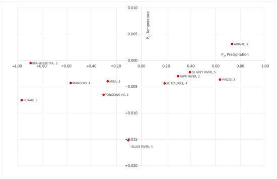
Figure 8.
A picture of polarisation phenomena in the area of precipitation and temperature, taking into account WMO regions.
Table 7.
Trend values of P2 polarisation components at 5% significance level for precipitation and temperature.
The concordance of the sign of the trend (RANGE) and trend (STD) for monthly precipitation and temperature is due to the fact that, in most cases, the variability in precipitation is correlated with changes in their maximum and minimum values. Similarly, in the area of temperature, the concordance of the sign of the trend (RANGE) and the trend (STD) for monthly temperatures is due to the fact that, in most cases, the variability in temperatures is correlated with changes in their maximum and minimum values. The characteristics of the river basins where polarisation was found in both the precipitation and temperature areas also included locations relating to Köppen–Geiger (K-G) classification areas [129,130].
The catchment area of the Mangoky River (Africa) is located on the island of Madagascar in the regions Bsh (arid, summer dry, hot arid) and Aw (equatorial, winter dry). It is characterised by negative values of both trends of precipitation polarisation factors and negative values of both trends of temperature polarisation factors. This indicates a decrease in the anomalies of precipitation and temperature factors. The decrease in the anomalies of precipitation factors while there is a decrease in temperature anomalies indicates a certain compatible relationship between the two factors in the catchment. This means that as precipitation anomalies decrease and stabilise, there may be a tendency toward lower temperatures or less extreme temperature changes.
The Yongding He River catchment is located in Asia in the Bsk (arid, dry summer) and Dwb (snow, dry winter and warm summer) regions. It is characterised by negative values of both trends of precipitation polarisation factors and negative values of both trends of temperature polarisation factors. This indicates a decrease in the anomalies of precipitation and temperature factors.
The catchment area of the Brahmaputra River is located in Asia in the regions: ET (polar, polar tundra) and Cwa (warm temperature, dry winter, hot summer). It is characterised by negative values of both trends of precipitation polarisation factors and negative values of both trends of temperature polarisation factors. This indicates a decrease in the anomalies of precipitation and temperature factors.
The Tapti River catchment is located in Asia in the Aw (equatorial, monsoonal) and As (equatorial, summer dry) regions. It is characterised by positive values of both trends of precipitation polarisation factors and negative values of both trends of temperature polarisation factors. This indicates an increase in precipitation factor anomalies with a decrease in temperature anomalies.
The Atrato River catchment is located in South America in the Af (equatorial, fully humid) region. It is characterised by positive values of both trends of precipitation polarisation factors and positive values of both trends of temperature polarisation factors. This indicates an increase in precipitation factor anomalies and temperature anomalies. If the region has positive values of both trends of precipitation polarisation factors and positive values of both trends of temperature polarisation factors, this indicates an increase in precipitation factor anomalies and temperature anomalies. Positive values of the precipitation polarisation factor trends suggest an increase in precipitation and greater variability in precipitation in the region. This could mean that precipitation becomes more abundant or more frequent and intense rainfall occurs. Positive trend values of temperature polarisation factors indicate an increase in temperature and greater temperature variability in the region.
The Mira River catchment is located in South America in the ET (polar, polar tundra) and Cfb (warm temperature, fully humid, warm summer) region. It is characterised by negative values of both trends of precipitation polarisation factors and negative values of both trends of temperature polarisation factors. This indicates a decrease in the anomalies of precipitation and temperature factors.
The Vinces River (South America) catchment is located at the boundary of the areas As (equatorial, dry summer), Am (equatorial, monsoonal), and Cfc (warm temperature, fully humid and cool summer). It is characterised by positive values of both trends of precipitation polarisation factors and negative values of both trends of temperature polarisation factors. This indicates an increase in precipitation factor anomalies with a decrease in temperature anomalies. This means that the amount of precipitation may be increasing or there may be more variability in precipitation in the area. In contrast, temperatures are less variable or stable, with decreasing temperature anomalies. An increase in precipitation factor anomalies while temperature anomalies are decreasing indicates a certain inverse relationship between the two factors in the catchment. This means that with higher precipitation, there may be a tendency towards lower temperatures or less extreme temperature changes.
The Ellice River catchment is located in North America, on the border of regions ET (polar, polar tundra) and Dfc (snow, fully humid, cool summer). It is characterised by negative values of both trends of precipitation polarisation factors and negative values of both trends of temperature polarisation factors. This indicates a decrease in the anomalies of precipitation and temperature factors.
The catchment area of the St. Maurice River is located in North America, on the border of the Dfb (snow, fully humid, cool summer) and Dfc (snow, fully humid, warm summer) regions. It is characterised by positive values of both precipitation polarisation factor trends and decreasing values of temperature polarisation factor trends. This indicates an increase in precipitation factor anomalies with a decrease in temperature anomalies.
The Purari River catchment is located in Australia and Oceania, in the Af (equatorial, fully humid) region. It is characterised by negative values of both trends of precipitation polarisation factors and negative values of both trends of temperature polarisation factors. This indicates a decrease in the anomalies of precipitation and temperature factors.
The De Grey River catchment is located in Australia and Oceania, in the Bwh (arid, winter dry, hot arid) region. It is characterised by positive values of both trends of precipitation polarisation factors and negative values of both trends of temperature polarisation factors. This indicates an increase in precipitation factor anomalies with a decrease in temperature anomalies.
Calming of precipitation and temperature anomalies (negative trends in both precipitation and temperature factors) are expected in the Brahmaputra and Yongding He catchments. For the Purari (Australia and Oceania) and Mangoky–Africa catchments, calculations indicate a calming of anomalies in both the temperature and precipitation variability area. Temperature and precipitation anomalies are to be expected in the Atrato River–South America catchments.
The analysis of K-G areas and catchments where trends in polarisation coefficients in both the area of monthly precipitation and monthly average temperatures have been recognised at the 5% significance level does not show associations of these catchment areas with the zones proposed by Köppen–Geiger [129,130].
In the calculations performed to determine the polarisation index, in addition to cases of trends with compatible signs (i.e., both positive and negative polarisation coefficients), there were also cases in which catchments showed opposite signs of polarisation coefficient trends in both precipitation and temperature sequence analysis. However, adopting a 5% significance level for the MKT resulted in the rejection of these cases. The concordance of the sign of the trend (max–min) and trend (STD) for precipitation is due to the fact that in most cases, the variability in precipitation is correlated with changes in its maximum and minimum values. In other words, when there are periods of increased precipitation, we usually also observe higher maximum and minimum values of precipitation, and thus an increase in variability relative to the average value. Similarly, when there are periods of increased drought, there are usually lower maximum and minimum precipitation values, and variability relative to the average is also lower. Note, however, that there are also periods in which maximum and minimum precipitation values may increase or decrease, but variability relative to the average remains constant or changes in the opposite direction.
9. Conclusions
This paper presents an analysis of monthly precipitation totals, based on the GPCC database, and monthly mean temperatures (NOAA data) for 377 catchments distributed worldwide, representing 12.76% of the Earth’s total surface area. The study covers a 110-year period from 1901 to 2010, using grid data with a spatial resolution of 0.5° × 0.5° latitude and longitude. Data were analysed in monthly intervals across the calendar year. In total, this study examined 377 catchments × 110 years × 12 months = 497,640 precipitation data series, and the same number of temperature data series, resulting in approximately one million long-term series that characterise climatic phenomena in terms of precipitation and temperature variability. Statistical characteristics for each calendar month were calculated, including minimum, maximum, and standard deviation values. Polarisation indices were computed based on the coefficients of amplitude and standard deviation, as well as the trends of these characteristics. Non-parametric Mann–Kendall Test (MKT) and Pettitt change-point test (PCPT) were used for trend analysis.
The analysis of monthly precipitation data across the catchments revealed that trends in the polarisation components (RANGE and STD) of monthly precipitation totals were confirmed at a 5% significance level in 25% of the catchments, while no significant trends were observed in the remaining 75%. Similarly, for the average monthly temperature data, trends in the polarisation coefficients were confirmed at a 5% significance level in 12.2% of the catchments, with no significant trends detected in the remaining 88.8%.
The analysis of temperature and precipitation polarisation is crucial due to its significant impact on various aspects of the natural and human environment. Based on long-term precipitation and temperature data, this paper demonstrates that polarisation processes are present and can lead to substantial changes in local environments. These changes may affect the distribution of plant and animal species, weather patterns, agriculture, the economy, and more. Moreover, precipitation and temperature variability play critical roles in global energy and water cycles, with potential consequences such as floods, droughts, and other natural disasters. Understanding the nature and timescales of these changes is essential for reducing the risk of extreme climate events such as droughts, heatwaves, heavy precipitation, flooding, or extreme cold.
A proper assessment of extreme event polarisation is vital for developing strategies to mitigate and minimise the impact of anthropogenic factors. Integrating adaptive and mitigative actions can help achieve long-term goals of balancing economic, social, and ecological needs. This paper presents methods for assessing the polarisation of precipitation and temperature variability, which can support the development of such strategies. Climate change trends suggest that polarisation is becoming more pronounced, with associated extremes intensifying and becoming more unevenly distributed. Analysing temperature and precipitation polarisation is critical for evaluating climate change and its environmental impacts, as well as for creating effective risk management strategies that minimise human impact on the environment, in line with the principles of sustainable development.
Funding
This research received no external funding.
Institutional Review Board Statement
This study did not require ethical approval.
Informed Consent Statement
Not applicable.
Data Availability Statement
The data presented in this study are available on request from the corresponding author. The data are not publicly available due to the size of the data structures.
Conflicts of Interest
The author declares no conflicts of interest.
References
- Romanowicz, R.J.; Bogdanowicz, E.; Debele, S.E.; Doroszkiewicz, J.; Hisdal, H.; Lawrence, D.; Meresa, H.K.; Napiórkowski, J.J.; Osuch, M.; Strupczewski, W.G.; et al. Climate Change Impact on Hydrological Extremes: Preliminary Results from the Polish-Norwegian Project. Acta Geophys. 2016, 64, 477–509. [Google Scholar] [CrossRef]
- Palaniswami, S.; Muthiah, K. Change Point Detection and Trend Analysis of Rainfall and Temperature Series over the Vellar River Basin. Polish J. Environ. Stud. 2018, 27, 1673–1682. [Google Scholar] [CrossRef] [PubMed]
- Groves, D.G.; Yates, D.; Tebaldi, C. Developing and Applying Uncertain Global Climate Change Projections for Regional Water Management Planning. Water Resour. Res. 2008, 44, 1–16. [Google Scholar] [CrossRef]
- Katz, R. Statistics of Extremes in Climatology and Hydrology. Adv. Water Resour. 2002, 25, 1287–1304. [Google Scholar] [CrossRef]
- Herschy, R.W. The World’s Maximum Observed Floods. Flow Meas. Instrum. 2002, 13, 231–235. [Google Scholar] [CrossRef]
- Blöschl, G.; Bierkens, M.F.P.; Chambel, A.; Cudennec, C.; Destouni, G.; Fiori, A.; Kirchner, J.W.; McDonnell, J.J.; Savenije, H.H.G.; Sivapalan, M.; et al. Twenty-Three Unsolved Problems in Hydrology (UPH)—A Community Perspective. Hydrol. Sci. J. 2019, 64, 1141–1158. [Google Scholar] [CrossRef]
- Lewis, S.C.; King, A.D. Evolution of Mean, Variance and Extremes in 21st Century Temperatures. Weather Clim. Extrem. 2017, 15, 1–10. [Google Scholar] [CrossRef]
- Jaiswal, R.K.; Lohani, A.K.; Tiwari, H.L. Statistical Analysis for Change Detection and Trend Assessment in Climatological Parameters. Environ. Process. 2015, 2, 729–749. [Google Scholar] [CrossRef]
- Heim, R.R. An Overview of Weather and Climate Extremes—Products and Trends. Weather Clim. Extrem. 2015, 10, 1–9. [Google Scholar] [CrossRef]
- Sillmann, J.; Thorarinsdottir, T.; Keenlyside, N.; Schaller, N.; Alexander, L.V.; Hegerl, G.; Seneviratne, S.I.; Vautard, R.; Zhang, X.; Zwiers, F.W. Understanding, Modeling and Predicting Weather and Climate Extremes: Challenges and Opportunities. Weather Clim. Extrem. 2017, 18, 65–74. [Google Scholar] [CrossRef]
- Młyński, D.; Cebulska, M.; Wałȩga, A. Trends, Variability, and Seasonality of Maximum Annual Daily Precipitation in the Upper Vistula Basin, Poland. Atmosphere 2018, 9, 313. [Google Scholar] [CrossRef]
- Młyński, D.; Wałȩga, A.; Petroselli, A.; Tauro, F.; Cebulska, M. Estimating Maximum Daily Precipitation in the Upper Vistula Basin, Poland. Atmosphere 2019, 10, 43. [Google Scholar] [CrossRef]
- Twardosz, R.C.M. Temporal Variability of Maximum Monthly Precipitation Totals in the Polish Western Carpathian Mts during the Period 1951–2005. Pr. Geogr. 2012, 128, 123–134. [Google Scholar] [CrossRef]
- Ziernicka-Wojtaszek, A.; Kopcińska, J. Variation in Atmospheric Precipitation in Poland in the Years 2001–2018. Atmosphere 2020, 11, 794. [Google Scholar] [CrossRef]
- Venegas-Cordero, N.; Kundzewicz, Z.W.; Jamro, S.; Piniewski, M. Detection of Trends in Observed River Floods in Poland. J. Hydrol. Reg. Stud. 2022, 41, 101098. [Google Scholar] [CrossRef]
- Kundzewicz, Z.W.; Radziejewski, M. Methodologies for Trend Detection. IAHS-AISH Publ. 2006, 308, 538–549. [Google Scholar]
- Kundzewicz, Z.W.; Robson, A. Detecting Trend and Other Changes in Hydrological Data. World Clim. Program.-Water 2000, 1013, 158. [Google Scholar]
- Berezowski, T.; Szczeniak, M.; Kardel, I.; Michalowski, R.; Okruszko, T.; Mezghani, A.; Piniewski, M. CPLFD-GDPT5: High-Resolution Gridded Daily Precipitation and Temperature Data Set for Two Largest Polish River Basins. Earth Syst. Sci. Data 2016, 8, 127–139. [Google Scholar] [CrossRef]
- Twaróg, B. Characteristics of Multi-Annual Variation of Precipitation in Areas Particularly Exposed to Extreme Phenomena. Part 1. the Upper Vistula River Basin. E3S Web Conf. 2018, 49, 00121. [Google Scholar] [CrossRef]
- Yu, Y.; He, F.; Vavrus, S.J.; Johnson, A.; Wu, H.; Zhang, W.; Yin, Q.; Ge, J.; Deng, C.; Petraglia, M.D.; et al. Climatic Factors and Human Population Changes in Eurasia between the Last Glacial Maximum and the Early Holocene. Glob. Planet. Change 2023, 221, 104054. [Google Scholar] [CrossRef]
- Chen, T.; Zou, L.; Xia, J.; Liu, H.; Wang, F. Decomposing the Impacts of Climate Change and Human Activities on Runoff Changes in the Yangtze River Basin: Insights from Regional Differences and Spatial Correlations of Multiple Factors. J. Hydrol. 2022, 615, 128649. [Google Scholar] [CrossRef]
- Szolgayova, E.; Parajka, J.; Blöschl, G.; Bucher, C. Long Term Variability of the Danube River Flow and Its Relation to Precipitation and Air Temperature. J. Hydrol. 2014, 519, 871–880. [Google Scholar] [CrossRef]
- Pechlivanidis, I.G.; Olsson, J.; Bosshard, T.; Sharma, D.; Sharma, K.C. Multi-Basin Modelling of Future Hydrological Fluxes in the Indian Subcontinent. Water 2016, 8, 177. [Google Scholar] [CrossRef]
- Mudelsee, M.; Börngen, M.; Tetzlaff, G.; Grünewald, U. Extreme Floods in Central Europe over the Past 500 Years: Role of Cyclone Pathway ‘Zugstrasse Vb’. J. Geophys. Res. D Atmos. 2004, 109, D23101. [Google Scholar] [CrossRef]
- Vavrus, S.J.; Notaro, M.; Lorenz, D.J. Interpreting Climate Model Projections of Extreme Weather Events. Weather Clim. Extrem. 2015, 10, 10–28. [Google Scholar] [CrossRef]
- Angélil, O.; Perkins-Kirkpatrick, S.; Alexander, L.V.; Stone, D.; Donat, M.G.; Wehner, M.; Shiogama, H.; Ciavarella, A.; Christidis, N. Comparing Regional Precipitation and Temperature Extremes in Climate Model and Reanalysis Products. Weather Clim. Extrem. 2016, 13, 35–43. [Google Scholar] [CrossRef]
- Michaelides, S.; Levizzani, V.; Anagnostou, E.; Bauer, P.; Kasparis, T.; Lane, J.E. Precipitation: Measurement, Remote Sensing, Climatology and Modeling. Atmos. Res. 2009, 94, 512–533. [Google Scholar] [CrossRef]
- Das, N.; Bhattacharjee, R.; Choubey, A.; Ohri, A.; Dwivedi, S.B.; Gaur, S. Time Series Analysis of Automated Surface Water Extraction and Thermal Pattern Variation over the Betwa River, India. Adv. Sp. Res. 2021, 68, 1761–1788. [Google Scholar] [CrossRef]
- Reinking, R.F. An Approach to Remote Sensing and Numerical Modeling of Orographic Clouds and Precipitation for Climatic Water Resources Assessment. Atmos. Res. 1995, 35, 349–367. [Google Scholar] [CrossRef]
- López-Bermeo, C.; Montoya, R.D.; Caro-Lopera, F.J.; Díaz-García, J.A. Validation of the Accuracy of the CHIRPS Precipitation Dataset at Representing Climate Variability in a Tropical Mountainous Region of South America. Phys. Chem. Earth Parts A/B/C 2022, 127, 103184. [Google Scholar] [CrossRef]
- Becker, A.; Finger, P.; Meyer-Christoffer, A.; Rudolf, B.; Schamm, K.; Schneider, U.; Ziese, M. A Description of the Global Land-Surface Precipitation Data Products of the Global Precipitation Climatology Centre with Sample Applications Including Centennial (Trend) Analysis from 1901-Present. Earth Syst. Sci. Data 2013, 5, 71–99. [Google Scholar] [CrossRef]
- Gómez, J.D.; Etchevers, J.D.; Monterroso, A.I.; Gay, C.; Campo, J.; Martínez, M. Spatial Estimation of Mean Temperature and Precipitation in Areas of Scarce Meteorological Information. Atmosfera 2008, 21, 35–56. [Google Scholar]
- Easterling, D.R.; Kunkel, K.E.; Wehner, M.F.; Sun, L. Detection and Attribution of Climate Extremes in the Observed Record. Weather Clim. Extrem. 2016, 11, 17–27. [Google Scholar] [CrossRef]
- Guimares Nobre, G.; Jongman, B.; Aerts, J.; Ward, P.J. The Role of Climate Variability in Extreme Floods in Europe. Environ. Res. Lett. 2017, 12, 084012. [Google Scholar] [CrossRef]
- Petrow, T.; Merz, B. Trends in Flood Magnitude, Frequency and Seasonality in Germany in the Period 1951–2002. J. Hydrol. 2009, 371, 129–141. [Google Scholar] [CrossRef]
- Singh, P.; Gupta, A.; Singh, M. Hydrological Inferences from Watershed Analysis for Water Resource Management Using Remote Sensing and GIS Techniques. Egypt. J. Remote Sens. Sp. Sci. 2014, 17, 111–121. [Google Scholar] [CrossRef]
- Zhang, X.; Vincent, L.A.; Hogg, W.D.; Niitsoo, A. Temperature and Precipitation Trends in Canada during the 20th Century. Atmos.-Ocean 2000, 38, 395–429. [Google Scholar] [CrossRef]
- Karmeshu, N. Trend Detection in Annual Temperature & Precipitation Using the Mann Kendall Test—A Case Study to Assess Climate Change on Select States in the Northeastern United States. Mausam 2015, 66, 1–6. [Google Scholar]
- Dankers, R.; Hiederer, R. Extreme Temperatures and Precipitation in Europe: Analysis of a High-Resolution Climate Change Scenario. JRC Sci. Tech. Rep. 2008, EUR 23291, 82. Available online: https://www.semanticscholar.org/paper/Extreme-Temperatures-and-Precipitation-in-Europe%3A-a-Rutger-Roland/05a831272412d5e53311e230bf171ff5f63f1751 (accessed on 14 April 2023).
- Katz, R.W.; Parlange, M.B. Overdispersion Phenomenon in Stochastic Modeling of Precipitation. J. Clim. 1998, 11, 591–601. [Google Scholar] [CrossRef]
- Roy, S.S.; Balling, R.C. Trends in Extreme Daily Precipitation Indices in India. Int. J. Climatol. 2004, 24, 457–466. [Google Scholar] [CrossRef]
- Colmet-Daage, A.; Sanchez-Gomez, E.; Ricci, S.; Llovel, C.; Estupina, V.B.; Quintana-Seguí, P.; Carmen Llasat, M.; Servat, E. Evaluation of Uncertainties in Mean and Extreme Precipitation under Climate Change for Northwestern Mediterranean Watersheds from High-Resolution Med and Euro-CORDEX Ensembles. Hydrol. Earth Syst. Sci. 2018, 22, 673–687. [Google Scholar] [CrossRef]
- Bernstein, L.; Bosch, P.; Canziani, O.; Chen, Z.; Christ, R.; Davidson, O.; Hare, W.; Huq, S.; Karoly, D.; Kattsov, V.; et al. Climate Change 2007: An Assessment of the Intergovernmental Panel on Climate Change. Change 2007, 446, 12–17. [Google Scholar]
- Pitt, M.A. Increased Temperature and Entropy Production in the Earth’s Atmosphere: Effect on Wind, Precipitation, Chemical Reactions, Freezing and Melting of Ice and Electrical Activity. J. Mod. Phys. 2019, 10, 966–973. [Google Scholar] [CrossRef]
- Knoben, W.J.M.; Woods, R.A.; Freer, J.E. Global Bimodal Precipitation Seasonality: A Systematic Overview. Int. J. Climatol. 2019, 39, 558–567. [Google Scholar] [CrossRef]
- WMO Guide to Climatological Practices 2018 Edition; WMO: Geneva, Switzerland, 2018; ISBN 9789263101006.
- Ross, S.M. Introduction to Probability and Statistics; Elsevier: Amsterdam, The Netherlands, 2014; ISBN 978-0-12-394811-3. [Google Scholar]
- Hao, Z. Application of Entropy Theory in Hydrologic Analysis and Simulation. Ph.D. Thesis, Texas A&M University, College Station, TX, USA, May 2016. [Google Scholar]
- Rica, C. Tropical Meteorology Research Programme (Tmrp) Commission for Atmospheric Sciences (CAS). Int. Organ. 2006, 16, 241–243. [Google Scholar] [CrossRef]
- Kuhlman, T.; Farrington, J. What Is Sustainability? Sustainability 2010, 2, 3436–3448. [Google Scholar] [CrossRef]
- Eizenberg, E.; Jabareen, Y. Social Sustainability: A New Conceptual Framework. Sustainability 2017, 9, 68. [Google Scholar] [CrossRef]
- McCormick, K.; Kautto, N. The Bioeconomy in Europe: An Overview. Sustainability 2013, 5, 2589–2608. [Google Scholar] [CrossRef]
- Velten, S.; Leventon, J.; Jager, N.; Newig, J. What Is Sustainable Agriculture? A Systematic Review. Sustainability 2015, 7, 7833–7865. [Google Scholar] [CrossRef]
- Lewandowski, M. Designing the Business Models for Circular Economy-towards the Conceptual Framework. Sustainability 2016, 8, 43. [Google Scholar] [CrossRef]
- Staffas, L.; Gustavsson, M.; McCormick, K. Strategies and Policies for the Bioeconomy and Bio-Based Economy: An Analysis of Official National Approaches. Sustainability 2013, 5, 2751–2769. [Google Scholar] [CrossRef]
- Müller, J.M.; Kiel, D.; Voigt, K.I. What Drives the Implementation of Industry 4.0? The Role of Opportunities and Challenges in the Context of Sustainability. Sustainability 2018, 10, 247. [Google Scholar] [CrossRef]
- Lahti, T.; Wincent, J.; Parida, V. A Definition and Theoretical Review of the Circular Economy, Value Creation, and Sustainable Business Models: Where Are We Now and Where Should Research Move in the Future? Sustainability 2018, 10, 2799. [Google Scholar] [CrossRef]
- Schaubroeck, T.; Schaubroeck, S.; Heijungs, R.; Zamagni, A.; Brandão, M.; Benetto, E. Attributional & Consequential Life Cycle Assessment: Definitions, Conceptual Characteristics and Modelling Restrictions. Sustainability 2021, 13, 7386. [Google Scholar] [CrossRef]
- Chapman, J. A Nonparametric Approach to Detecting Changes in Variance in Locally Stationary Time Series. Environmetrics 2020, 31, e2576. [Google Scholar] [CrossRef]
- Thornton, P.K.; Ericksen, P.J.; Herrero, M.; Challinor, A.J. Climate Variability and Vulnerability to Climate Change: A Review. Glob. Change Biol. 2014, 20, 3313–3328. [Google Scholar] [CrossRef]
- Swanson, K.L.; Tsonis, A.A. Has the Climate Recently Shifted? Geophys. Res. Lett. 2009, 36, L06711. [Google Scholar] [CrossRef]
- Balhane, S.; Driouech, F.; Chafki, O.; Manzanas, R.; Chehbouni, A.; Moufouma-Okia, W. Changes in Mean and Extreme Temperature and Precipitation Events from Different Weighted Multi-Model Ensembles over the Northern Half of Morocco. Clim. Dyn. 2022, 58, 389–404. [Google Scholar] [CrossRef]
- Mesbahzadeh, T.; Miglietta, M.M.; Mirakbari, M.; Soleimani Sardoo, F.; Abdolhoseini, M. Joint Modeling of Precipitation and Temperature Using Copula Theory for Current and Future Prediction under Climate Change Scenarios in Arid Lands (Case Study, Kerman Province, Iran). Adv. Meteorol. 2019, 2019, 6848049. [Google Scholar] [CrossRef]
- Gerten, D.; Rost, S.; von Bloh, W.; Lucht, W. Causes of Change in 20th Century Global River Discharge. Geophys. Res. Lett. 2008, 35, 1–5. [Google Scholar] [CrossRef]
- Walling, D.E. Human Impact on Land–Ocean Sediment Transfer by the World’s Rivers. Geomorphology 2006, 79, 192–216. [Google Scholar] [CrossRef]
- Hunter, T.S.; Clites, A.H.; Campbell, K.B.; Gronewold, A.D. Development and Application of a North American Great Lakes Hydrometeorological Database—Part I: Precipitation, Evaporation, Runoff, and Air Temperature. J. Great Lakes Res. 2015, 41, 65–77. [Google Scholar] [CrossRef]
- Chai, Y.; Yue, Y.; Zhang, L.; Miao, C.; Borthwick, A.G.L.; Zhu, B.; Li, Y.; Dolman, A.J. Homogenization and Polarization of the Seasonal Water Discharge of Global Rivers in Response to Climatic and Anthropogenic Effects. Sci. Total Environ. 2020, 709, 136062. [Google Scholar] [CrossRef] [PubMed]
- Li, Z.; Shi, Y.; Argiriou, A.A.; Ioannidis, P.; Mamara, A.; Yan, Z. A Comparative Analysis of Changes in Temperature and Precipitation Extremes since 1960 between China and Greece. Atmosphere 2022, 13, 1824. [Google Scholar] [CrossRef]
- Jahn, M. Economics of Extreme Weather Events: Terminology and Regional Impact Models. Weather Clim. Extrem. 2015, 10, 29–39. [Google Scholar] [CrossRef]
- Zhang, X.; Alexander, L.; Hegerl, G.C.; Jones, P.; Tank, A.K.; Peterson, T.C.; Trewin, B.; Zwiers, F.W. Indices for Monitoring Changes in Extremes Based on Daily Temperature and Precipitation Data. Wiley Interdiscip. Rev. Clim. Change 2011, 2, 851–870. [Google Scholar] [CrossRef]
- Allan, R.P.; Soden, B.J. Atmospheric Warming and the Amplification of Precipitation Extremes. Science 2008, 321, 1481–1484. [Google Scholar] [CrossRef]
- Christensen, J.H.; Kanikicharla, K.K.; Aldrian, E.; An, S.I.; Albuquerque Cavalcanti, I.F.; de Castro, M.; Dong, W.; Goswami, P.; Hall, A.; Kanyanga, J.K.; et al. Climate Phenomena and Their Relevance for Future Regional Climate Change. In Climate Change 2013—The Physical Science Basis; Working Group I Contribution to the Fifth Assessment Report of the Intergovernmental Panel on Climate Change; Cambridge University Press: Cambridge, UK, 2013; Volume 9781107057, pp. 1217–1308. [Google Scholar] [CrossRef]
- Cardona, O.D.; Van Aalst, M.K.; Birkmann, J.; Fordham, M.; Mc Gregor, G.; Rosa, P.; Pulwarty, R.S.; Schipper, E.L.F.; Sinh, B.T.; Décamps, H.; et al. Determinants of Risk: Exposure and Vulnerability. In Managing the Risks of Extreme Events and Disasters to Advance Climate Change Adaptation; Special Report of the Intergovernmental Panel on Climate Change; Cambridge University Press: Cambridge, UK, 2012; Volume 9781107025, pp. 65–108. [Google Scholar] [CrossRef]
- Kolokytha, E.; Oishi, S.; Teegavarapu, R.S.V. Sustainable Water Resources Planning and Management under Climate Change; Kolokytha, E., Ed.; Springer Science+Business Media: Singapore, 2016; ISBN 9789811020513. [Google Scholar]
- Powell, J.P.; Reinhard, S. Measuring the Effects of Extreme Weather Events on Yields. Weather Clim. Extrem. 2015, 12, 69–79. [Google Scholar] [CrossRef]
- Lal, P.N.; Mitchell, T.; Aldunce, P.; Auld, H.; Mechler, R.; Miyan, A.; Romano, L.E.; Zakaria, S.; Dlugolecki, A.; Masumoto, T.; et al. National Systems for Managing the Risks from Climate Extremes and Disasters; Cambridge University Press: Cambridge, UK, 2012; Volume 9781107025, ISBN 9781139177245. [Google Scholar]
- Knapp, A.K.; Beier, C.; Briske, D.D.; Classen, A.T.; Yiqi, L.; Reichstein, M.; Smith, M.D.; Smith, S.D.; Bell, J.E.; Fay, P.A.; et al. Consequences of More Extreme Precipitation Regimes for Terrestrial Ecosystems. Bioscience 2008, 58, 811–821. [Google Scholar] [CrossRef]
- Sitthiyot, T.; Holasut, K. A Simple Method for Measuring Inequality. Palgrave Commun. 2020, 6, 112. [Google Scholar] [CrossRef]
- Vermeulen, S.J.; Challinor, A.J.; Thornton, P.K.; Campbell, B.M.; Eriyagama, N.; Vervoort, J.M.; Kinyangi, J.; Jarvis, A.; Läderach, P.; Ramirez-Villegas, J.; et al. Addressing Uncertainty in Adaptation Planning for Agriculture. Proc. Natl. Acad. Sci. USA 2013, 110, 8357–8362. [Google Scholar] [CrossRef] [PubMed]
- Ramirez-Villegas, J.; Lau, C.; Köhler, A.K.; Signer, J.; Jarvis, A.; Arnell, N.W.; Osborne, T.M.; Hooker, J. Climate Analogues: Finding Tomorrow’s Agriculture Today. Work. Pap. No. 12 2011, 12, 40. [Google Scholar]
- Matos, S.; Viardot, E.; Sovacool, B.K.; Geels, F.W.; Xiong, Y. Innovation and Climate Change: A Review and Introduction to the Special Issue. Technovation 2022, 117, 102612. [Google Scholar] [CrossRef]
- Pfleiderer, P.; Schleussner, C.F.; Mengel, M.; Rogelj, J. Global Mean Temperature Indicators Linked to Warming Levels Avoiding Climate Risks. Environ. Res. Lett. 2018, 13, 059501. [Google Scholar] [CrossRef]
- Stephan, G. Intergenerational Fairness and Climate Change Adaptation Policy: An Economic Analysis. Green Low-Carbon Econ. 2023, 1, 105–109. [Google Scholar] [CrossRef]
- Langdon, J.G.R.; Lawler, J.J. Assessing the Impacts of Projected Climate Change on Biodiversity in the Protected Areas of Western North America. Ecosphere 2015, 6, 1–14. [Google Scholar] [CrossRef]
- Nicolli, F.; Gilli, M.; Vona, F. Inequality and Climate Change: Two Problems, One Solution. Fond. Eni Enrico Mattei Inequal. 2023. [Google Scholar] [CrossRef]
- Twaróg, B. Application of Shannon Entropy in Precipitation Conditions and Application of Shannon Entropy in Assessing Changes in Precipitation Conditions and Temperature Based on Long-Term Sequences Using the Bootstrap Method. Atmosphere 2024, 15, 898. [Google Scholar] [CrossRef]
- Hosseinzadehtalaei, P.; Tabari, H.; Willems, P. Climate Change Impact on Short-Duration Extreme Precipitation and Intensity–Duration–Frequency Curves over Europe. J. Hydrol. 2020, 590, 125249. [Google Scholar] [CrossRef]
- Persson, J.; Blennow, K.; Gonçalves, L.; Borys, A.; Dutca, I.; Hynynen, J.; Janeczko, E.; Lyubenova, M.; Martel, S.; Merganic, J.; et al. No Polarization-Expected Values of Climate Change Impacts among European Forest Professionals and Scientists. Sustainability 2020, 12, 2659. [Google Scholar] [CrossRef]
- Rudolf, B.; Beck, C.; Grieser, J.; Schneider, U. Global Precipitation Analysis Products of the GPCC. Internet Publ. 2005, 112, 3819–3837. [Google Scholar]
- Arheimer, B.; Pimentel, R.; Isberg, K.; Crochemore, L.; Andersson, J.C.M.; Hasan, A.; Pineda, L. Global Catchment Modelling Using World-Wide HYPE (WWH), Open Data, and Stepwise Parameter Estimation. Hydrol. Earth Syst. Sci. 2020, 24, 535–559. [Google Scholar] [CrossRef]
- Iverson, L.R.; McKenzie, D. Tree-Species Range Shifts in a Changing Climate: Detecting, Modeling, Assisting. Landsc. Ecol. 2013, 28, 879–889. [Google Scholar] [CrossRef]
- Franklin, J. Mapping Species Distributions: Spatial Inference and Prediction. Oryx 2010, 44, 615. [Google Scholar] [CrossRef]
- Viner, D.; Ekstrom, M.; Hulbert, M.; Warner, N.K.; Wreford, A.; Zommers, Z. Understanding the Dynamic Nature of Risk in Climate Change Assessments—A New Starting Point for Discussion. Atmos. Sci. Lett. 2020, 21, e958. [Google Scholar] [CrossRef]
- Rosenzweig, C.; Parry, M. Potential Impact of Climate Change on World Food Supply. Nature 1992, 367, 133–138. [Google Scholar] [CrossRef]
- Tabari, H.; Willems, P. Lagged Influence of Atlantic and Pacific Climate Patterns on European Extreme Precipitation. Sci. Rep. 2018, 8, 5748. [Google Scholar] [CrossRef]
- Gibbins, G.; Haigh, J.D. Entropy Production Rates of the Climate. J. Atmos. Sci. 2020, 77, 3551–3566. [Google Scholar] [CrossRef]
- Kharin, V.V.; Zwiers, F.W.; Zhang, X.; Wehner, M. Changes in Temperature and Precipitation Extremes in the CMIP5 Ensemble. Clim. Change 2013, 119, 345–357. [Google Scholar] [CrossRef]
- Verstraeten, G.; Poesen, J.; Demarée, G.; Salles, C. Long-Term (105 Years) Variability in Rain Erosivity as Derived from 10-Min Rainfall Depth Data for Ukkel (Brussels, Belgium): Implications for Assessing Soil Erosion Rates. J. Geophys. Res. Atmos. 2006, 111, 1–11. [Google Scholar] [CrossRef]
- Lovell, R.S.L.; Blackburn, T.M.; Dyer, E.E.; Pigot, A.L. Environmental Resistance Predicts the Spread of Alien Species. Nat. Ecol. Evol. 2021, 5, 322–329. [Google Scholar] [CrossRef] [PubMed]
- Stocker, T.F.; Clarke, G.K.C.; Le Treut, H.; Lindzen, R.S.; Meleshko, V.P.; Mugara, R.K.; Palmer, T.N.; Pierrehumbert, R.T.; Sellers, P.J.; Trenberth, K.E.; et al. Physical Climate Processes and Feedbacks. In Climate Change 2001: The Scientific Basis; Contribution of Working Group I to the Third Assessment Report of the Intergovernmental Panel on Climate Change; Cambridge University Press: Cambridge, UK, 2001; Volume 881, pp. 419–457. [Google Scholar]
- Chen, L.; Guo, S. Copulas and Its Application in Hydrology and Water Resources; Springer: Singapore, 2019; ISBN 978-981-13-0573-3. [Google Scholar]
- Hou, W.; Yan, P.; Feng, G.; Zuo, D. A 3D Copula Method for the Impact and Risk Assessment of Drought Disaster and an Example Application. Front. Phys. 2021, 9, 656253. [Google Scholar] [CrossRef]
- Santos-Gómez, J.D.; Fontalvo-García, J.S.; Giraldo Osorio, J.D. Validating the University of Delaware’s Precipitation and Temperature Database for Northern South America. Dyna 2015, 82, 86–95. [Google Scholar] [CrossRef]
- Amiel, Y.; Cowell, F. Thinking about Inequality; Cambridge University Press: Cambridge, UK; New York, NY, USA, 1999; ISBN 9780511492266. [Google Scholar]
- Lorenz, M.O. Methods of Measuring the Concentration of Wealth. Publ. Am. Stat. Assoc. 1905, 9, 209–219. [Google Scholar] [CrossRef]
- Mccright, A.M.; Dunlap, R.E. The Politicization of Climate Change and Polarization in the American Public’s Views of Global Warming, 2001–2010. Sociol. Q. 2011, 52, 155–194. [Google Scholar] [CrossRef]
- Ogwang, T. Calculating a Standard Error for the Gini Coefficient: Some Further Results: Reply. Oxf. Bull. Econ. Stat. 2004, 66, 435–437. [Google Scholar] [CrossRef]
- Damgaard, C.; Weiner, J. Describing Inequality in Plant Size or Fecundity. Ecology 2000, 81, 1139. [Google Scholar] [CrossRef]
- Panek, T. Polaryzacja Ekonomiczna w Polsce. Wiadomości. Stat. 2017, 1, 41–62. [Google Scholar]
- Samson, P.-M. Concentration of Measure Principle and Entropy-Inequalities; Springer: New York, NY, USA, 2017; ISBN 9781493970049. [Google Scholar]
- Yitzhaki, S. Gini’s Mean Difference: A Superior Measure of Variability for Non-Normal Gini’s Mean Difference: A Superior Measure of Variability for Non-Normal Distributions. Metron. Lxi 2016, 2, 285–316. [Google Scholar]
- Conceição, P.; Ferreira, P. Young Person’s Guide to the Theil Index: Suggesting Intuitive Interpretations and Exploring Analytical Applications. World 2000, 1–54. [Google Scholar] [CrossRef]
- Buishand, T.A. Some Methods for Testing the Homogeneity of Rainfall Records. J. Hydrol. 1982, 58, 11–27. [Google Scholar] [CrossRef]
- Chen, J.; Gupta, A.K. Parametric Statistical Change Point Analysis. 2013–2015. Angew. Chemie Int. Ed. 2021, 6, 951–952. [Google Scholar] [CrossRef]
- Radziejewski, M.; Bardossy, A.; Kundzewicz, Z.W. Detection of Change in River Flow Using Phase Randomization. Hydrol. Sci. J. 2000, 45, 547–558. [Google Scholar] [CrossRef]
- Salarijazi, M. Trend and Change-Point Detection for the Annual Stream-Flow Series of the Karun River at the Ahvaz Hydrometric Station. African J. Agric. Res. 2012, 7, 4540–4552. [Google Scholar] [CrossRef]
- Pettitt, A.N. A Non-Parametric Approach to the Change-Point Problem. J. R. Stat. Soc. Ser. C Appl. Stat. 1979, 28, 126–135. [Google Scholar] [CrossRef]
- Conte, L.C.; Bayer, D.M.; Bayer, F.M. Bootstrap Pettitt Test for Detecting Change Points in Hydroclimatological Data: Case Study of Itaipu Hydroelectric Plant, Brazil. Hydrol. Sci. J. 2019, 64, 1312–1326. [Google Scholar] [CrossRef]
- Mann, H.B. Nonparametric Tests Against Trend. Econometrica 1945, 13, 245–259. [Google Scholar] [CrossRef]
- Yue, S.; Pilon, P.; Phinney, B.; Cavadias, G. The Influence of Autocorrelation on the Ability to Detect Trend in Hydrological Series. Hydrol. Process. 2002, 16, 1807–1829. [Google Scholar] [CrossRef]
- Sen, P.K. Estimates of the Regression Coefficient Based on Kendall’s Tau. J. Am. Stat. Assoc. 1968, 63, 1379–1389. [Google Scholar] [CrossRef]
- Hirsch, R.M.; Slack, J.R.; Smith, R.A. Techniques of Trend Analysis for Monthly Water Quality Data. Water Resour. Res. 1982, 18, 107–121. [Google Scholar] [CrossRef]
- Production and Consumption Gross Energy Consumption by Source. Available online: https://statice.is/statistics/environment/energy/production-and-consumption/ (accessed on 14 April 2023).
- Everett, K.; Hardick, E.; Johnson, D. The Year of Africa; The African Presence; The Ohio State University: Columbus, OH, USA, 2018; pp. 1–24. [Google Scholar] [CrossRef]
- Khanin, G.I. The 1950s: The Triumph of the Soviet Economy. Eur. Asia. Stud. 2003, 55, 1187–1211. [Google Scholar] [CrossRef]
- Levy, M.; Stewart, D.E.; Kent, C.H.W. Encyclopedia Britannica. 2023, pp. 1–15. Available online: https://www.britannica.com/topic/Encyclopaedia-Britannica-English-language-reference-work (accessed on 14 April 2024).
- Love, J.L. The Rise and Decline of Economic Structuralism in Latin America: New Dimensions. Lat. Am. Res. Rev. 2023, 40, 100–125. [Google Scholar] [CrossRef]
- van Eck, C.W.; Mulder, B.C.; Dewulf, A. Online Climate Change Polarization: Interactional Framing Analysis of Climate Change Blog Comments. Sci. Commun. 2020, 42, 454–480. [Google Scholar] [CrossRef]
- Beck, H.E.; Zimmermann, N.E.; McVicar, T.R.; Vergopolan, N.; Berg, A.; Wood, E.F. Present and Future Köppen-Geiger Climate Classification Maps at 1-Km Resolution. Sci. Data 2018, 5, 180214. [Google Scholar] [CrossRef]
- Kottek, M.; Grieser, J.; Beck, C.; Rudolf, B.; Rubel, F. World Map of the Köppen-Geiger Climate Classification Updated. Meteorol. Z. 2006, 15, 259–263. [Google Scholar] [CrossRef] [PubMed]
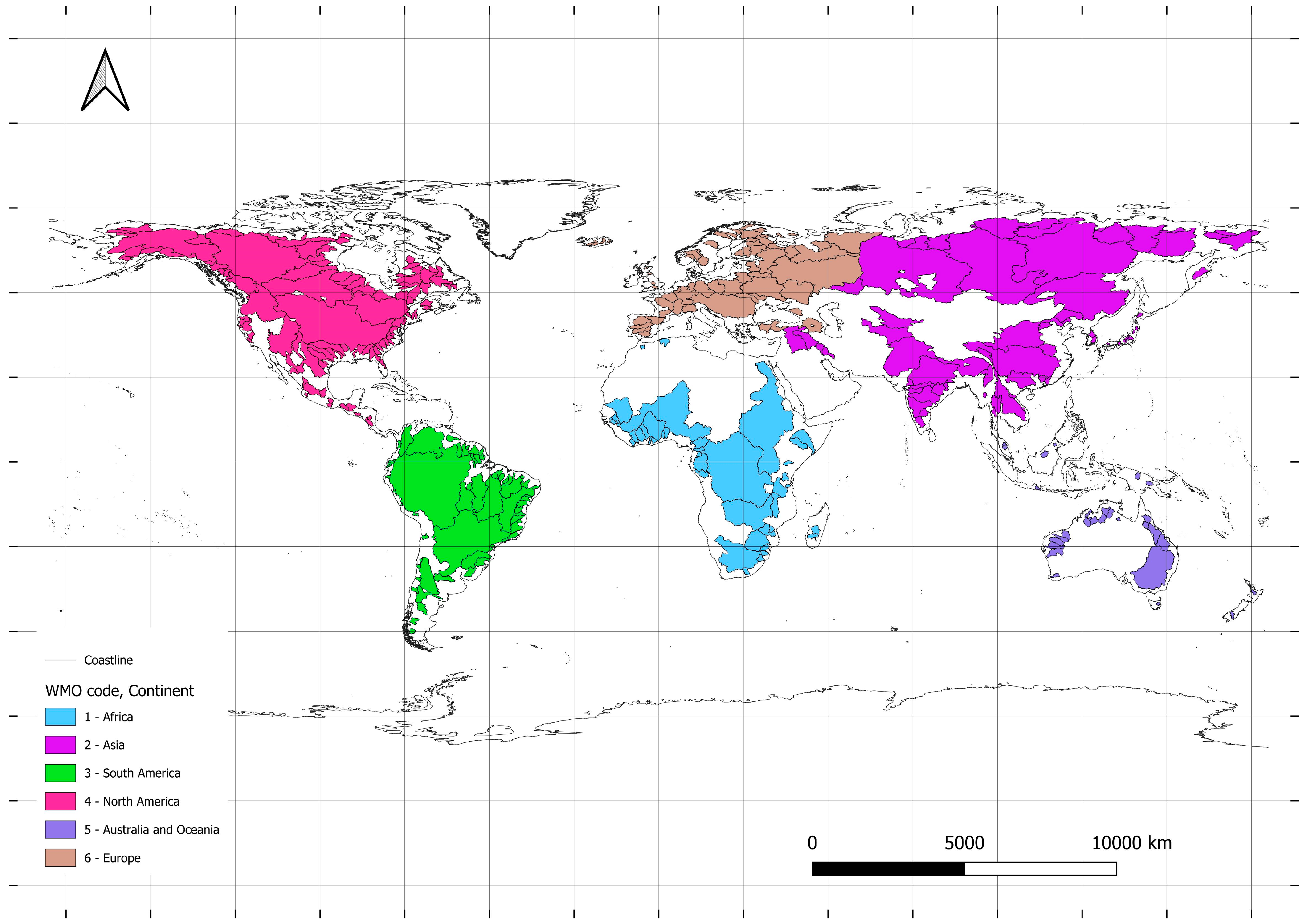
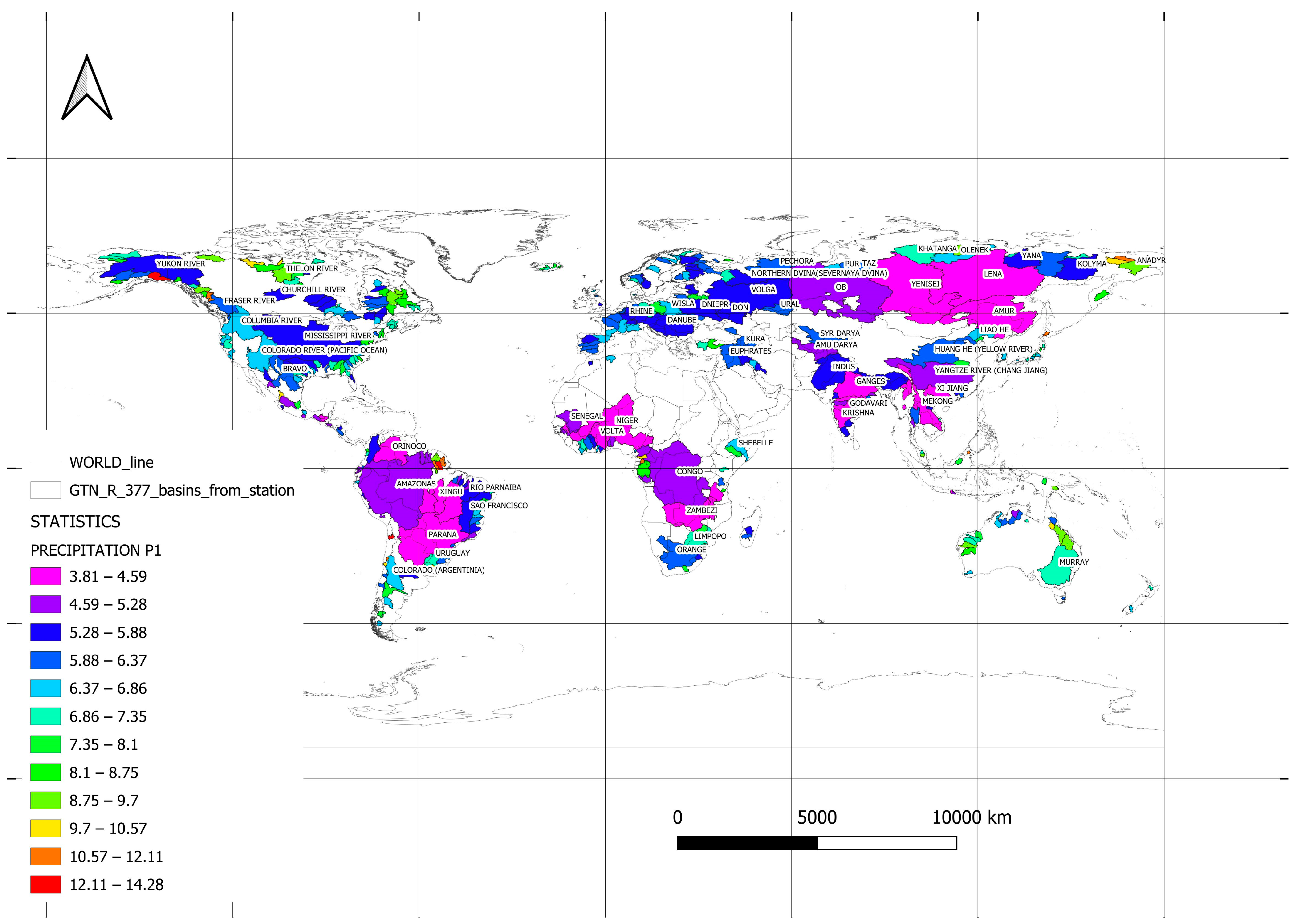
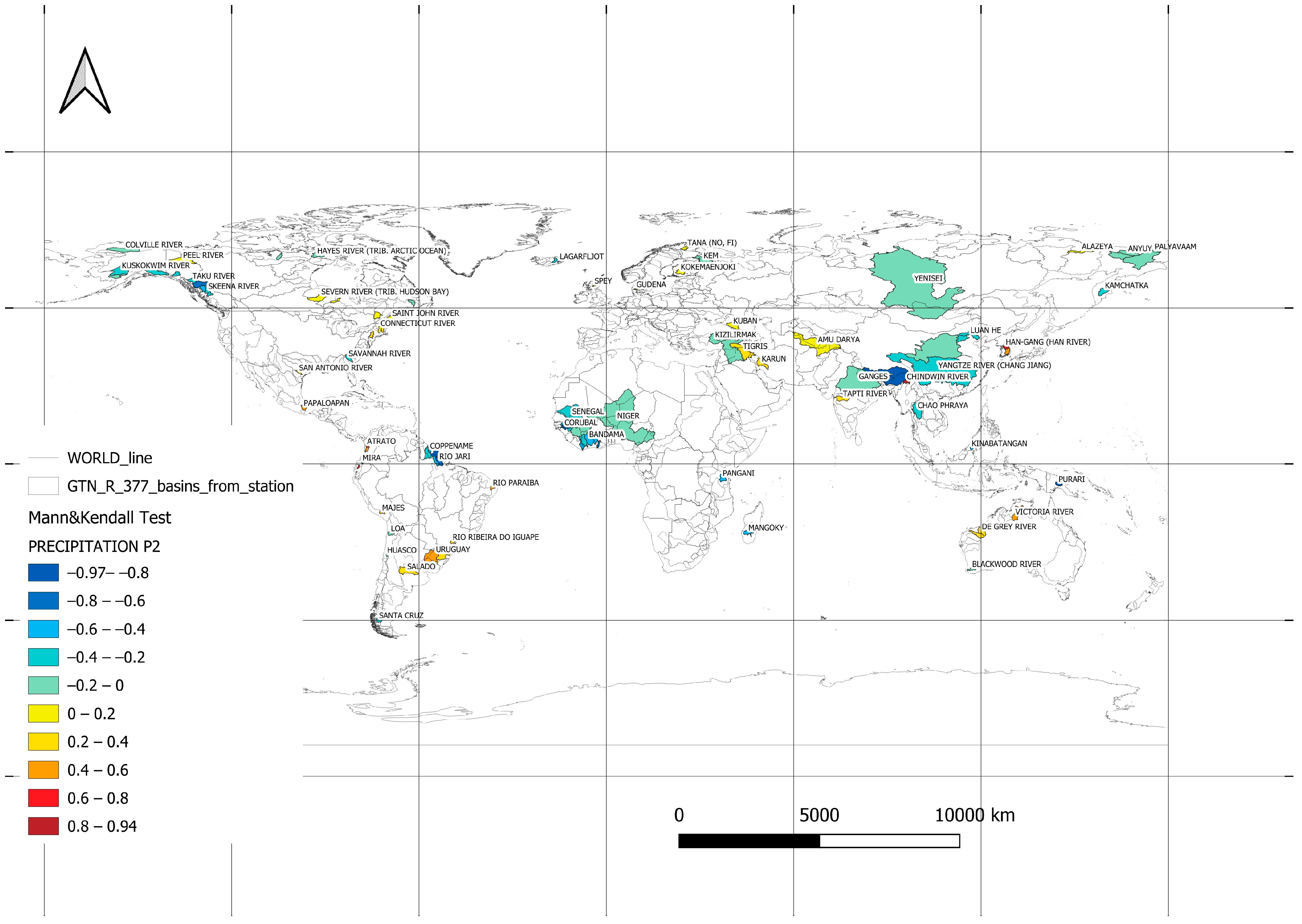
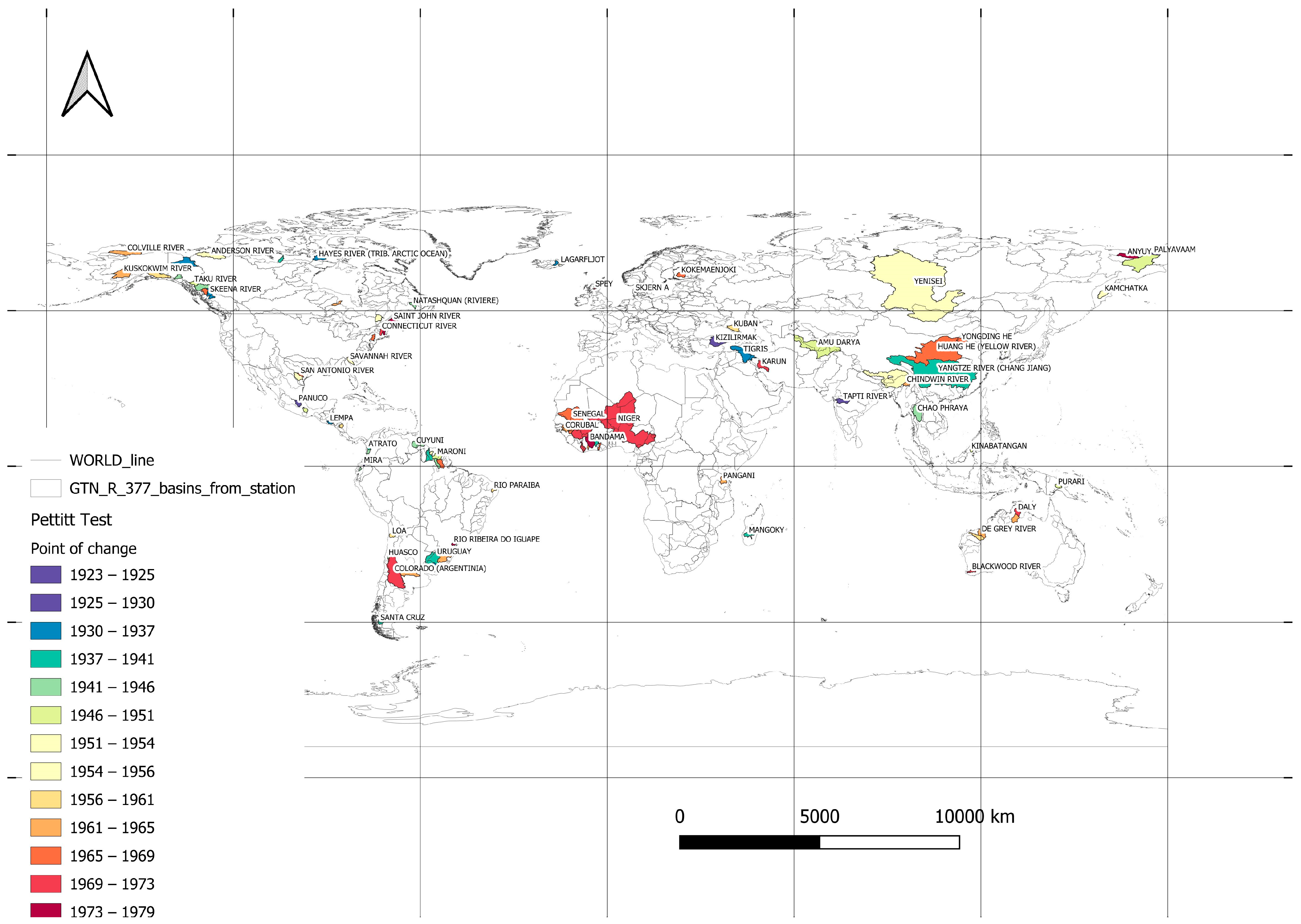
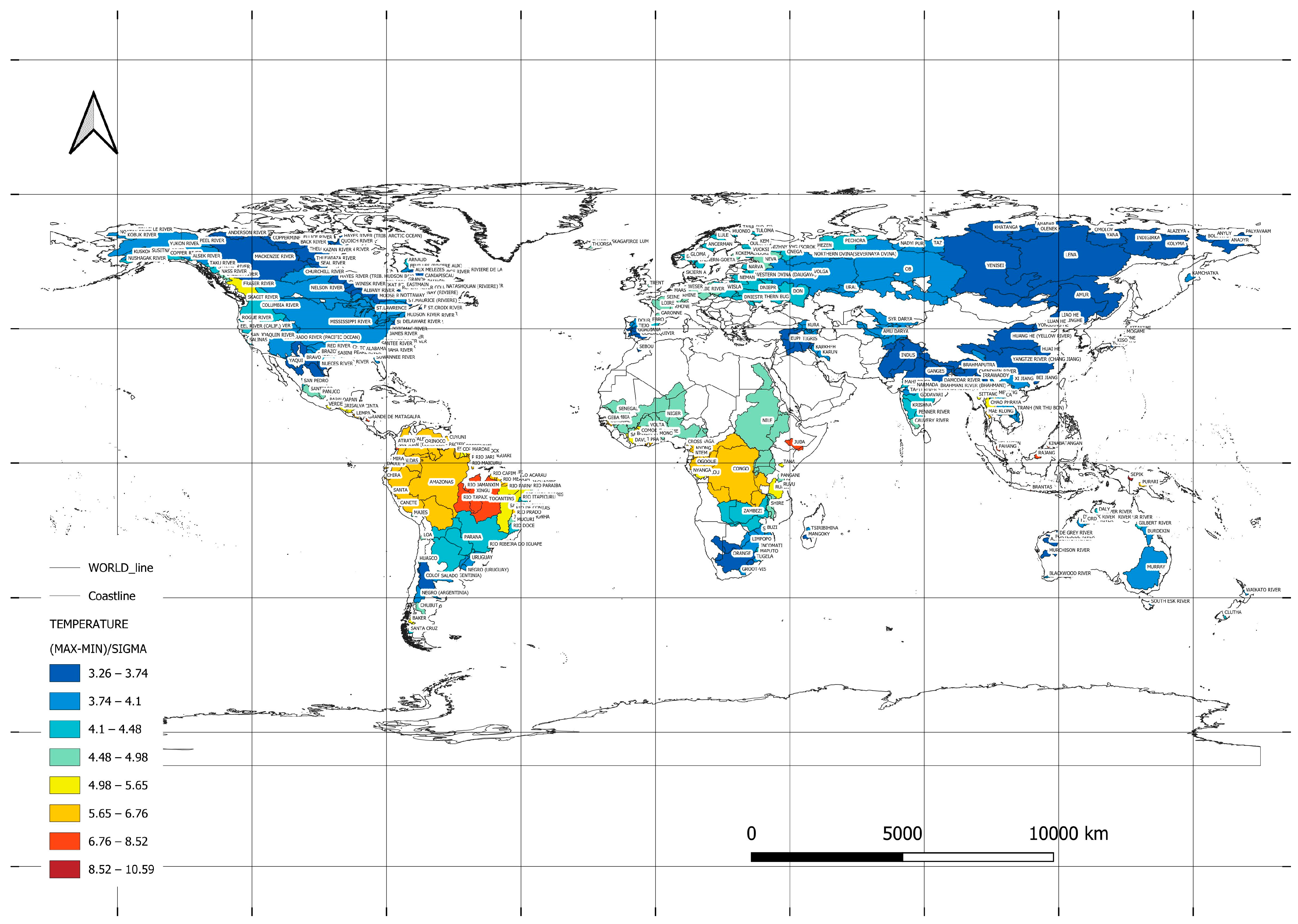
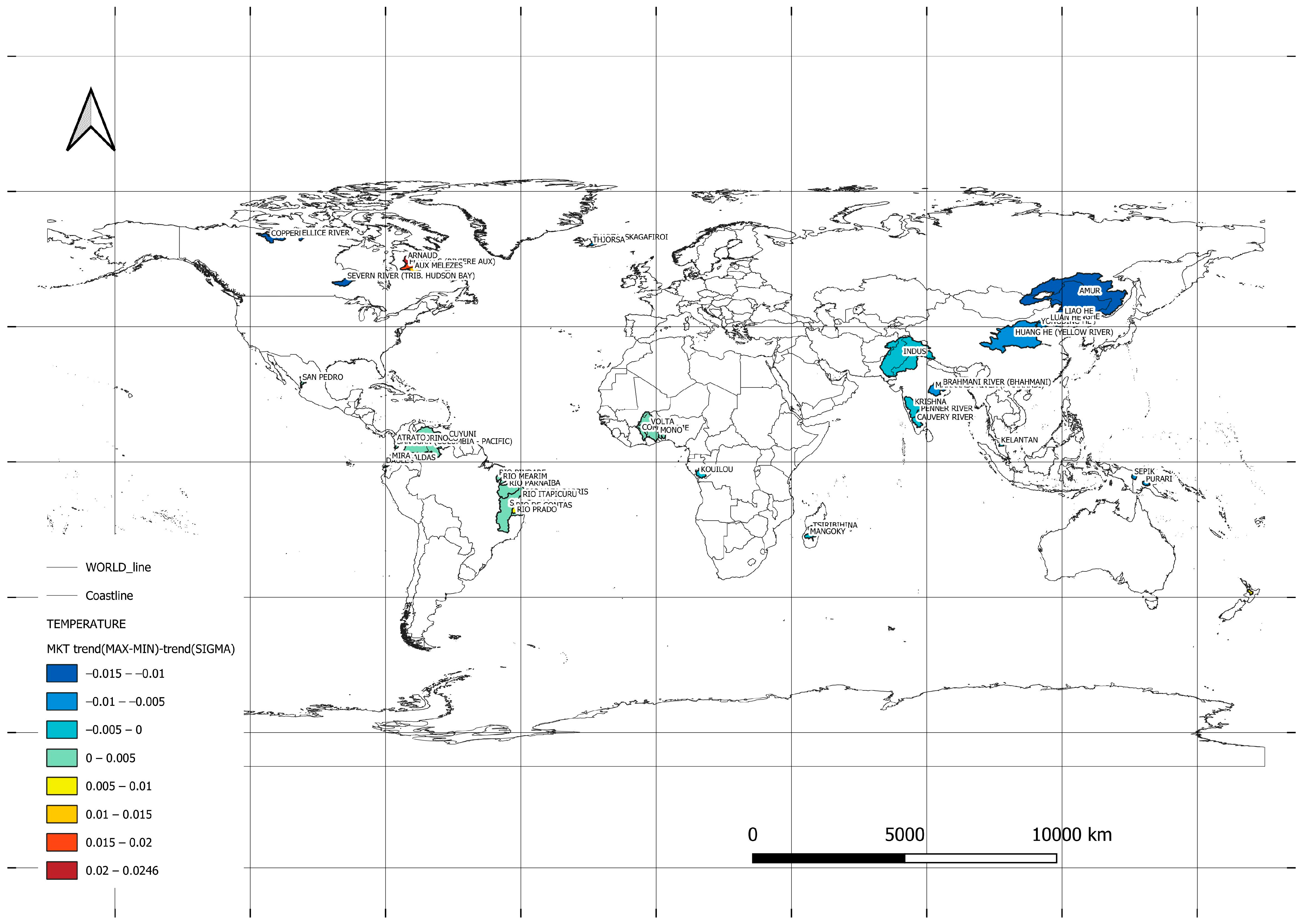
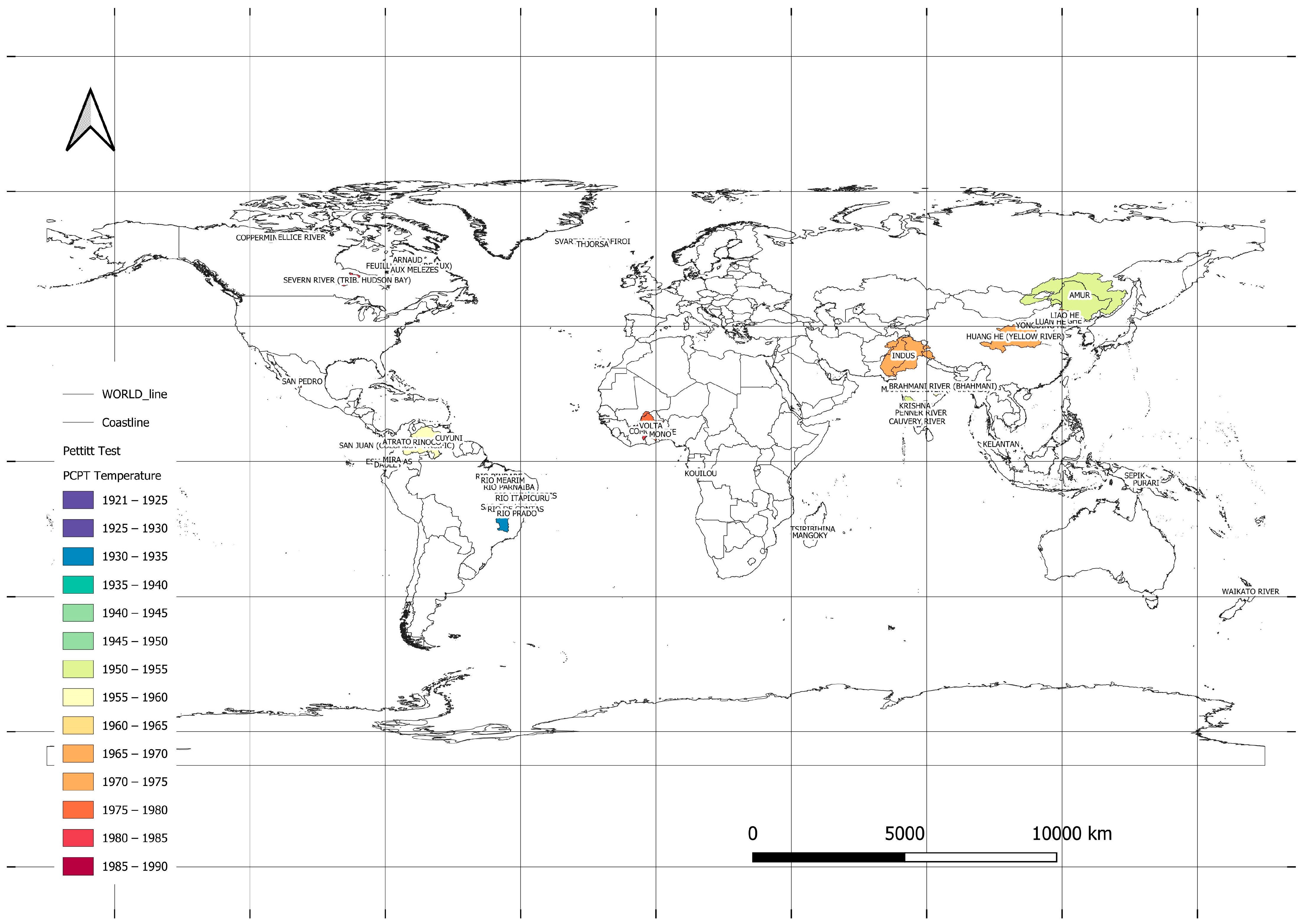
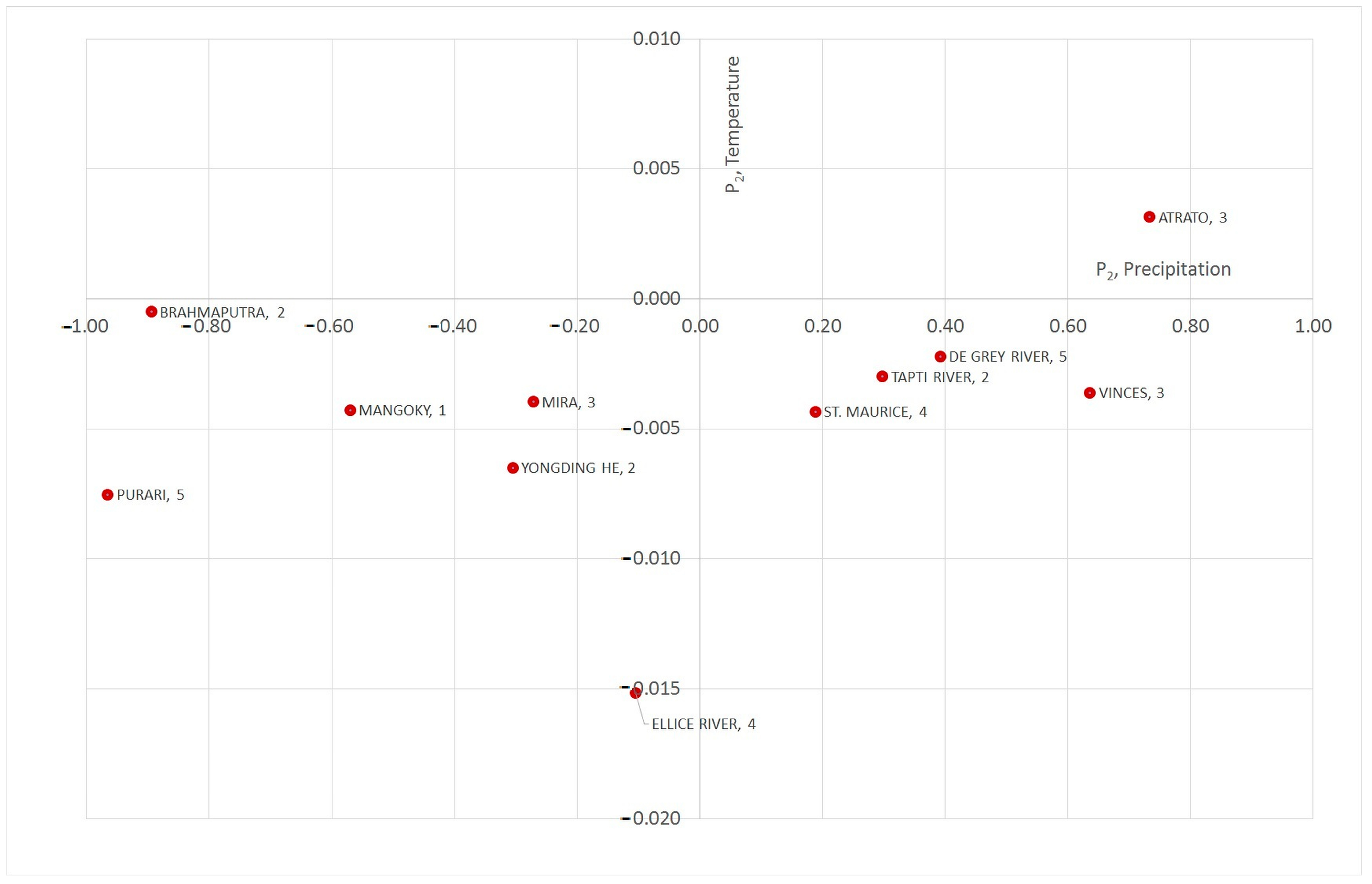
Disclaimer/Publisher’s Note: The statements, opinions and data contained in all publications are solely those of the individual author(s) and contributor(s) and not of MDPI and/or the editor(s). MDPI and/or the editor(s) disclaim responsibility for any injury to people or property resulting from any ideas, methods, instructions or products referred to in the content. |
© 2024 by the author. Licensee MDPI, Basel, Switzerland. This article is an open access article distributed under the terms and conditions of the Creative Commons Attribution (CC BY) license (https://creativecommons.org/licenses/by/4.0/).