Abstract
Most machine learning (ML) studies on predicting co-seismic landslides have relied on Peak Ground Acceleration (PGA). The PGA of the ground strongly correlates with the relative position and azimuth of the seismogenic faults. Using the co-seismic landslide records of the 2008 Wenchuan earthquake, we show that the ML model using the distances and azimuths from the epicenter to sites performs better than the PGA model regarding accuracy and actual prediction results. The distances and azimuths are more accessible than the PGA because obtaining accurate and realistic large-scale PGAs is difficult. Considering their computational efficiency and cost-effectiveness, the ML models utilizing distances and azimuths from the epicenter to the sites as inputs could be an alternative to PGA-based models for evaluating the impact of co-seismic landslides. Notably, these models prove advantageous in near-real-time scenarios and settings requiring high spatial resolution, and provide favorable assistance in achieving the goal of sustainable development of society.
1. Introduction
Landslides are a natural hazard when earth, debris, and rocks slide down a slope due to gravity [1,2]. The ground shaking during earthquakes induces instability, leading to these gravitational movements [3]. Co-seismic landslides, as secondary hazards of earthquakes, can cause significant damage to human life, infrastructure, and the economy [1]. Moreover, the displacement of masses triggered by landslides can result in the formation of dammed lakes or floods, posing risks to downstream urban areas [4,5]. Consequently, the efficient and rapid assessment of the impact area of post-earthquake landslides is crucial, particularly in urban expansion.
Predicting landslides is a complex task due to the significant variability in ground materials and surface conditions, often observed over short distances [6]. There are many challenges in predicting co-seismic landslides, and one of the most important challenges is the uncertainty of the seismic characteristics. Previous studies have commonly employed empirical or numerical simulation methods to estimate landslide patterns. Empirical methods involve establishing statistical correlations between landslide occurrences and various factors, such as slope, rock type, and rainfall, to facilitate predictive modeling [6]. Malamud, et al. [3] introduced a landslide-event magnitude scale, which provides a valuable framework for understanding the frequency-area distribution of landslides in landslide research. Following the Wenchuan earthquake in the year 2008, Gorum, et al. [7] investigated the correlation between landslides and related conditioning factors. Hungr and McDougall [8] developed two numerical models to simulate landslide runouts. Traditional landslide hazard risk analysis has frequently relied on statistical approaches. Carrara et al. [9] utilized statistical models and stepwise discriminant analysis to evaluate landslide hazards in central Italy. Lee et al. [10] proposed a statistical approach to assess the susceptibility of earthquake-triggered landslides. Since around 2000, researchers have started to use logistic regression for landslide hazard assessment [11]. Xu et al. [12] compared six machine learning models to map landslides triggered by the 2008 Wenchuan earthquake, incorporating eleven geological and topographical factors.
In recent studies, machine learning has emerged as a widely adopted approach for landslide susceptibility assessment. For example, Tien Bui et al. [13] employed support vector machines, artificial neural networks, kernel logistic regression, and logistic tree models to predict landslide hazards in Vietnam. Dou et al. [14] applied Random Forest and decision tree models for landslide susceptibility mapping in Japan. Merghadi et al. [15] conducted a comprehensive analysis of various machine-learning methods and found that the Random Forest algorithm exhibited excellent performance in mapping landslide susceptibility. Consistent results were reported by Dou et al. [14], highlighting the rapid and accurate generation of landslide susceptibility maps by the Random Forest model. Fan et al. [16] achieved significant progress in the near-real-time prediction of co-seismic landslide distribution by leveraging a dataset of 0.3 million landslides and incorporating multiple geological and topographical information as inputs. Liu et al. [17] demonstrated satisfactory performance in mapping landslide susceptibility using convolutional neural network (CNN)-based models. Sun et al. [18] found that the SVM model using multiple landslide conditioning factors to map the susceptibility to geological hazards in the Changbai Mountain region affected by volcanic activity gave good results. Wang et al. [19] introduced swap noise as an unsupervised mechanism to improve the generalization performance and transferability of the model, reduce false alarms, and improve accuracy through supervised fine-tuning. Su et al. [20] used several models such as a Backpropagation Neural Network (BPNN), Residual Neural Network (ResNet), Convolutional Neural Network (CNN), and Visual Geometry Group-16 (VGG-16) for landslide hazard assessment, and the results showed that the Inception model performed the best in rainfall-induced landslide susceptibility assessment.
The occurrence of landslides resulting from earthquakes is highly complex, influenced by factors such as geomorphology, geology, and vegetation cover. However, the primary driver of co-seismic landslides is seismic dynamics. While several studies have explored the use of machine learning for predicting co-seismic landslides, many of them rely on seismic dynamic factors such as Peak Ground Acceleration (PGA), seismic intensity, distance from the epicenter, and distance from the probable seismogenic fault [7,16,21,22,23,24,25,26,27,28,29]. PGA is generally considered one of the most crucial factors contributing to co-seismic landslides [12,21,27,28,30,31]. In practical applications, PGA is often used as an input parameter for machine learning models due to limited information on near-source observations and the spatial distribution of seismic faults. However, there are difficulties in obtaining real PGAs on a large scale. Empirically regressed ground-motion prediction equations (GMPEs) are commonly employed to predict ground motion, including PGA and peak ground velocity (PGV), based on a simple hypothesis. The ground shaking estimated by these equations may differ from the actual ground shaking conditions due to problems associated with the ergodic assumption and the incomplete incorporation of spatial correlation and constraints in empirical GMPEs [32].
This study aims to use distances and azimuths from the epicenter to sites as inputs into machine learning instead of PGA to achieve a more concise, faster, and economical way to accomplish the prediction. For an earthquake (e.g., the 2008 Wenchuan earthquake we discuss in this work), the ground motion at the site is mainly affected by the propagation path of seismic waves from the earthquake fault to the site. These effects can be mainly clarified as two critical parameters: the azimuth and epicentral distance. As the seismic wave spreads and propagates in 3D space, its energy and amplitude decay with the distance from the source [33]. The epicentral distance is a primary parameter to evaluate ground motion intensity in GMPE. Another critical factor is the azimuth of the size referring to the earthquake fault. Note that the azimuth is not considered in the traditional GMPE method when evaluating ground motion, as the method implemented a homogeneous seismic wave propagation pattern [34,35]. However, ground motion distributions are highly heterogeneous in observations and forward simulations [36,37]. Compared to other models, this paper’s innovative contribution is the use of easily obtained distances and azimuths to replace the difficult-to-obtain and potentially error-prone PGAs as inputs to assess co-seismic landslides.
Predicting co-seismic landslides is crucial for assessing seismic hazards, and this method enhances machine learning algorithms for landslide prediction, aiding seismic hazard mitigation and prevention [38]. The methodology proposed in this paper can contribute to local and global sustainable development goals. The subsequent sections will outline our approach to forecasting co-seismic landslides in the study area. Furthermore, we will comprehensively compare four prediction models based on varying inputs. Finally, this paper discusses the significant role distance and azimuth play from the epicenter to the site in this study.
2. Methods and Data
2.1. Modeling Approach
The objective of our model is to estimate the distribution probability of co-seismic landslides. The overview presented in Figure 1 summarizes the main steps of estimation procedure. Initially, we collected the data of earthquake-triggered landslides and various factors (Step 1). This study’s 12 factors are derived from topographical, geological, and seismic data (Step 1). These factors include elevation, slope, aspect, Terrain Ruggedness Index (TRI), distance to faults and water lines, soil type, lithology, landform, peak ground acceleration (PGA), and the distance and azimuth from the epicenter to the site (Step 2). We joined these data with the same spatial position alongside the corresponding landslide or non-landslide status (Step 3). Subsequently, a machine learning model used these data to give the probability estimation of co-seismic landslides (Steps 4 and 5). The outputs generated by these models provide valuable feedback for further improvement (Step 5).
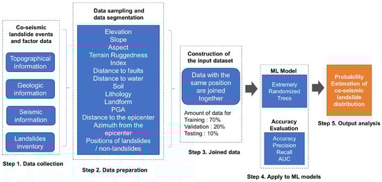
Figure 1.
The overview of the estimation procedure of the distribution probability of co-seismic landslides. Twelve landslide-related factors are applied to an Extremely Randomized Trees model to predict co-seismic landslides.
2.2. Model Performance Assessment
A confusion matrix is a table layout that allows the visualization of the performance of a predictive model [39]. In the confusion matrix, the true positive (TP) and the true negative (TN) are the numbers of correctly classified grids. Meanwhile, the false positive (FP) and the false negative (FN) are numbers of grids that are classified incorrectly.
Accuracy is the ratio of correctly predicted landslide grids and non-landslide grids (TP and TN) in all input data (TP + FP + FN + TN) in Equation (1) [39]. Accuracy reflects the model’s overall ability for binary classifications. Precision is a proportion of correctly predicted landslides grids (TP) in all predicted landslides grids (TP + FP) in Equation (2), and Recall means the proposition of correctly predicted landslides grids (TP) in all observation landslides grids (TP + FN) in Equation (3) [39]. Precision and Recall represent the model’s ability to identify landslides.
Receiver operating characteristics (ROC) curves help visualize model performance and select classifiers [40]. The area under the ROC curve (AUC) is a single scalar value to measure the classifier’s performance [41].
2.3. Extremely Randomized Trees
The Extremely Randomized Trees (ERT) model is one of the best-suited models for decision-making in landslide susceptibility mapping, and exhibits superior performance compared to other models [15]. The ERT machine learning model can reduce overfitting and increase efficiency. ERT is similar to the Random Forest model. The core idea of the ERT model is to increase the stochasticity of the model, thereby reducing the variance of the model and improving generalization. ERT models split the tree nodes through random attribution and cut-point choices, and have a unrelated output structure from the learning samples [42]. Compared with the Random Forest model, ERT has better computational efficiency with a similar accuracy [42]. The ERT method has three steps: splitting nodes, picking a random split, and stopping splitting if the split is smaller than a specific size. The parameters , , and correspond to the three steps described above. The parameter stands for the number of random splits based on attribute differences. The is the number of samples required for splitting a node. The represents the number of trees in the ensemble. The ERT node splitting procedure starts by importing all selected independent variables into the ERT model and randomly selecting attributes. Then, the procedure will generate splits randomly and construct many extra trees with these splits. Those trees will finally establish the extra tree ensemble [43]. Table 1 concludes the key parameters of the training algorithm for this study. The model and kernel can be defined as [42]:
and
where is a learning sample of size , and is a tree structure with leaves. Therefore, is the characteristic function of the leaf of , by the number of learning samples , such that , and we defined as the vector of (normalized) characteristic functions of t [42]:

Table 1.
A summary of key parameters for model training.
2.4. Study Area and Data
2.4.1. Overview of the Study Area
The M 7.9 Wenchuan earthquake occurred on 12 May 2008 in the marginal zone between Longmen Mountain and the Sichuan Basin. This event caused loss of life, with 69,227 fatalities, 17,923 individuals reported as missing, and 374,643 people injured. The earthquake also caused extensive destruction to countless infrastructures and civilian buildings [26]. Longmen Shan’s uplift resulted from the northward subduction of the Indian plate beneath the Eurasian plate. The eastward expansion of the Tibetan Plateau played a critical role in triggering the Wenchuan earthquake, as the Tibetan Plateau exerted pressure against the Sichuan Basin [44].
The study area is located within the earthquake-affected region of Sichuan province in southwestern China. It is a square region measuring approximately 110 km in length and width, spanning from 103° to 104° E longitude and 31° to 32° N latitude. The study area is near Chengdu city, as indicated by the blue frame in Figure 2. Figure 2 provides a historical overview of earthquake events in this area dating back to 1900. In the study area, co-seismic landslides are primarily concentrated in the complex mountainous terrain, encompassing numerous active faults. The precise epicenter of the Wenchuan earthquake is located at co-ordinates 31.002° N and 103.322° E, denoted by the red star in Figure 2 (USGS).
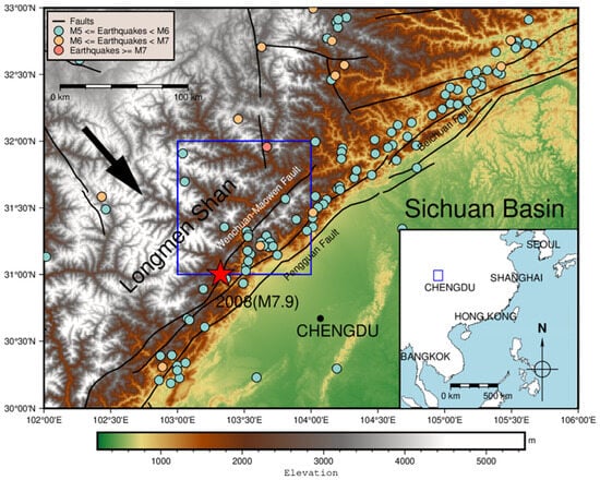
Figure 2.
The seismological background of the study area. Due to the movement of the Tibetan Plateau (black arrow), many active faults (data and resources) can be observed in this region [45,46]. Historical earthquake records (USGS, since 1900) show high seismic activities along the Pengguan and Beichuan faults. The red star represents the epicenter of the 2008 Wenchuan Earthquake.
2.4.2. Landslide Data
Using high-resolution aerial photographs, Xu et al. [27] collected a comprehensive inventory of landslides triggered by the 2008 Wenchuan earthquake. This inventory consists of 197,481 polygons that accurately depict the sizes and geometries of each co-seismic landslide resulting from the earthquake. The total area of landslides in this inventory is approximately 1160 km2. For our study, we utilize this landslide inventory to demonstrate the application of our proposed machine-learning model.
2.4.3. Environmental Factor Data
Empirical evidence suggests that co-seismic landslides are influenced by multiple factors, including elevation, slope, aspect, topographic relief index (TRI), soil type, lithology, landform, distance to faults, distances to hydrographic networks, distance and azimuth from the epicenter to the site, and peak ground acceleration (PGA). The factors, including the aspect, Terrain Ruggedness Index, distance to faults, distance to water, distance to the epicenter, and azimuth from the epicenter are calculated by QGis. Our research incorporates all the factors above to investigate the relationship between landslides and earthquakes. It is important to note that all the information used in this study is publicly available and accessible.
Table 2 gives the classification of possible co-seismic landslide factors. Seismic factors include PGA, distance to faults, distance to the epicenter, and azimuth angle from the epicenter. As shown in Figure 3, most of the co-seismic landslide area is PGA 0.6~0.9 g (Figure 3A). The relationships between landslide and distance to faults and epicenter are shown in Figure 3B,C. More than 80% of the landslides were within 45 to 120 km of faults, and 10 to 90 km of the epicenter. About 60% of landslides have an azimuth angle from the epicenter within 30 to 60 degrees (Figure 3D).
Table 2.
Classification of the seismic, terrain, and geologic factors.
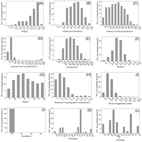
Figure 3.
Percentage (PCT.) of area for potential landslide-controlling factors. Twelve factors are classified into the seismic factors: (A) PGA, (B) distance to faults, (C) distance to the epicenter, and (D) azimuth from the epicenter; the terrain factors: (E) elevation, (F) slope angle, (G) slope aspect, (H) distance to hydrographic networks, (I) terrain ruggedness index, and (J) landforms; and the geologic factors: (K) soil types and (L) lithology.
Terrain factors include elevation, slope angle, slope aspect, distance to hydrographic networks, terrain ruggedness index (TRI), and landforms. Most landslides are between 1000 and 3500 m above sea level (Figure 3E) and have slopes between 20 and 50 degrees (Figure 3F). The landslides have the most east- (E) and southeast-oriented (SE) aspects (Figure 3G). Most landslides were within 10 km of the network (Figure 3H). A total of 70% of the landslides had a TRI of 30 to 90 (Figure 3I), and almost all landslides belonged to the high-gradient mountain class (TM) (Figure 3J).
Geologic factors are soil factors and rock factors. Geologic factors consist of soil factors and rock factors. More than 40% of the landslides in the study area are haplic luvisols (LVh) (Figure 3K). Meanwhile, slate, phyllite, and pellitic rock (MA3/MB1) account for most of the landslide area, followed by Eolian unconsolidated rocks (UE1) (Figure 3L).
2.5. Training, Validation, and Test Data
This study considers 13 distinct layers, including 12 conditioning factor maps and a landslide inventory map. These layers provide various information about the study area. To ensure uniformity in analysis, all layers were converted into a grid format with a resolution of 30 m by 30 m, allowing for consistent spatial co-ordinates across all layers. Each grid point represented a specific location and comprised data such as latitude, longitude, elevation, slope, aspect, topographic relief index (TRI), soil type, lithology, landform, peak ground acceleration (PGA), distance and azimuth from the epicenter to the site, distance to faults, distance to water lines, and a landslide or non-landslide status.
This study involves nearly 13 million points, with approximately 0.8 million points representing landslide occurrences and the remaining points representing non-landslide areas. Landslide points were assigned a value of “1”, while non-landslide points were assigned a value of “0”. To facilitate model development and evaluation, the collected data will be partitioned into training, validation, and testing datasets using a split ratio of 7:2:1. The training dataset will be used for constructing the model. In contrast, validation and testing datasets will be employed to assess the model’s performance and validate its results.
2.6. Different Model Construction Schemes
The study employed four machine-learning models, each utilizing different factors as inputs. The first model, ERT-A, utilized all 12 available factors to investigate the relationship between earthquakes and landslides. The second model, ERT-B, shared 11 factors with ERT-A, excluding peak ground acceleration (PGA) from its inputs. Similarly, the third model, ERT-C, leveraged ten factors from ERT-A but eliminated azimuth and distance variables to evaluate the impact of co-seismic landslides specifically. Lastly, the fourth model, ERT-D, employed the same factor inputs as ERT-A, excluding seismic factors. ERT-D focused on seven factors: elevation, slope, aspect, topographic relief index (TRI), soil type, lithology, and landform.
3. Results
3.1. Prediction Performance
The prediction results from four models are illustrated in Table 3. Except for ERT-D, all three models showed a similar performance in co-seismic landslide prediction and can had a good capacity for co-seismic landslide assessment.
Table 3.
Comparison of prediction results.
The results in Table 3 show that the ERT-B model performed similarly to the ERT-A model. The ERT-A model used geological, topographic, and seismic factors to predict landslides. Meanwhile, the ERT-B model used the same input except PGA information. These two models’ accuracy, recall, and AUC scores were over 0.90, and the precision scores were over 0.825. For comparison, the ERT-C model, which has input factors similar to those of the ERT-A model except for the distance and azimuth from the epicenter to the site, scored slightly lower in all categories than ERT-A and ERT-B. Specifically, ERT-C had an accuracy of under 0.9, a precision of under 0.825, a recall of under 0.88, and an AUC of under 0.96. The ERT-D model, which had inputs without seismic factors, had the worst performance.
The results indicate that the seismic factors are critical in these models. Earthquake-related factors play a dominant role in co-seismic landslide assessment. Moreover, the distance and azimuth from the epicenter to the site can replace PGA to predict co-seismic landslides. The two epicenter-related factors capture the impact of earthquake energy on the earth’s surface. If complete and credible PGA data are obtained, no significant difference exists between the PGA and the distance and azimuth between the epicenter and the site. However, often, there are missing PGA observations, and missing PGA data may result in landslide underestimates or overestimates. The results also indicate that the main factor inducing landslides after an earthquake is the destabilization of the existing loose material on the ground surface caused by the propagation of seismic energy to the ground surface. This argument, however, still requires an explanation of physical processes.
3.2. Landslides Prediction Results
Figure 4 illustrates the comparison of four estimated landslide results from various inputs. Only selected areas have been illustrated here to facilitate the presentation.
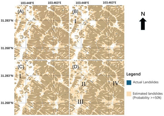
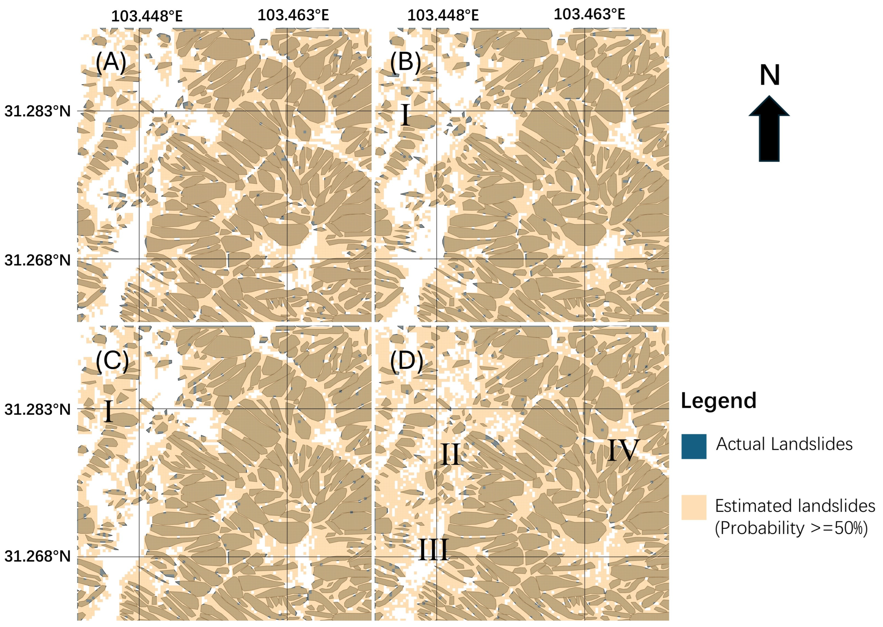
Figure 4.
The prediction outputs comparison using various input factors. The subplots (A–D) are obtained from ERT-A, ERT-B, ERT-C, and ERT-D, respectively. The polygons with black indicate the actual co-seismic landslide areas in the 2008 Wenchuan Earthquake. The yellow areas show estimated landslides (the predicted probabilities of landslides in yellow areas are greater than or equal to 50%). The regions around the Roman numerals in the figure will be discussed in the text.
Figure 4A–D are four estimated results from ERT-A, ERT-B, ERT-C, and ERT-D. The majority of the main characteristics of the spatial distribution of landslides and non-landslide areas have been captured in Figure 4A–C. The differences between the actual landslide extent and the predicted four outputs are relatively small. The predicted landslide clearly and accurately outlines the boundaries of the actual landslide.
The landslide prediction results in Figure 4A–C are noticeably better than those in Figure 4D. Figure 4A shows the output using all 12 factors. Figure 4B,C are the predicted landslide impact extent derived without the input of PGA and epicenter-related factors, respectively. Contrasting Region I in Figure 4B,C, the ERT-B model provides a more accurate prediction of the landslide area than the ERT-C model. This finding reflects that using epicenter correlation factors can more accurately characterize the landslide area than the PGA. Figure 4D shows the results obtained using the non-seismic factors. It needs a better prediction near Region II, III, and IV. Many non-landslide areas are misclassified as landslides. It indicates that seismic factors can play a significant role in predicting co-seismic landslide machine learning.
4. Discussion
Machine learning operations provide a valuable means to generate a landslide susceptibility map, enabling a more comprehensive understanding of landslide risk. Figure 5 presents a comparison of landslide susceptibilities obtained using different inputs.
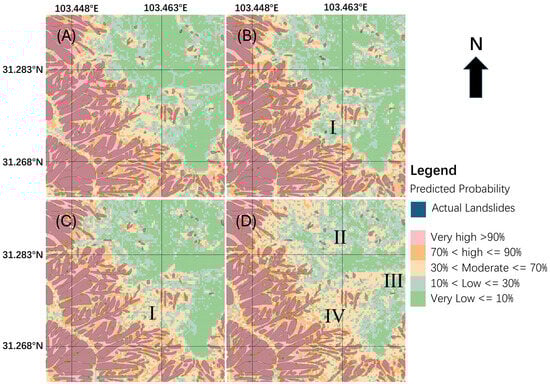
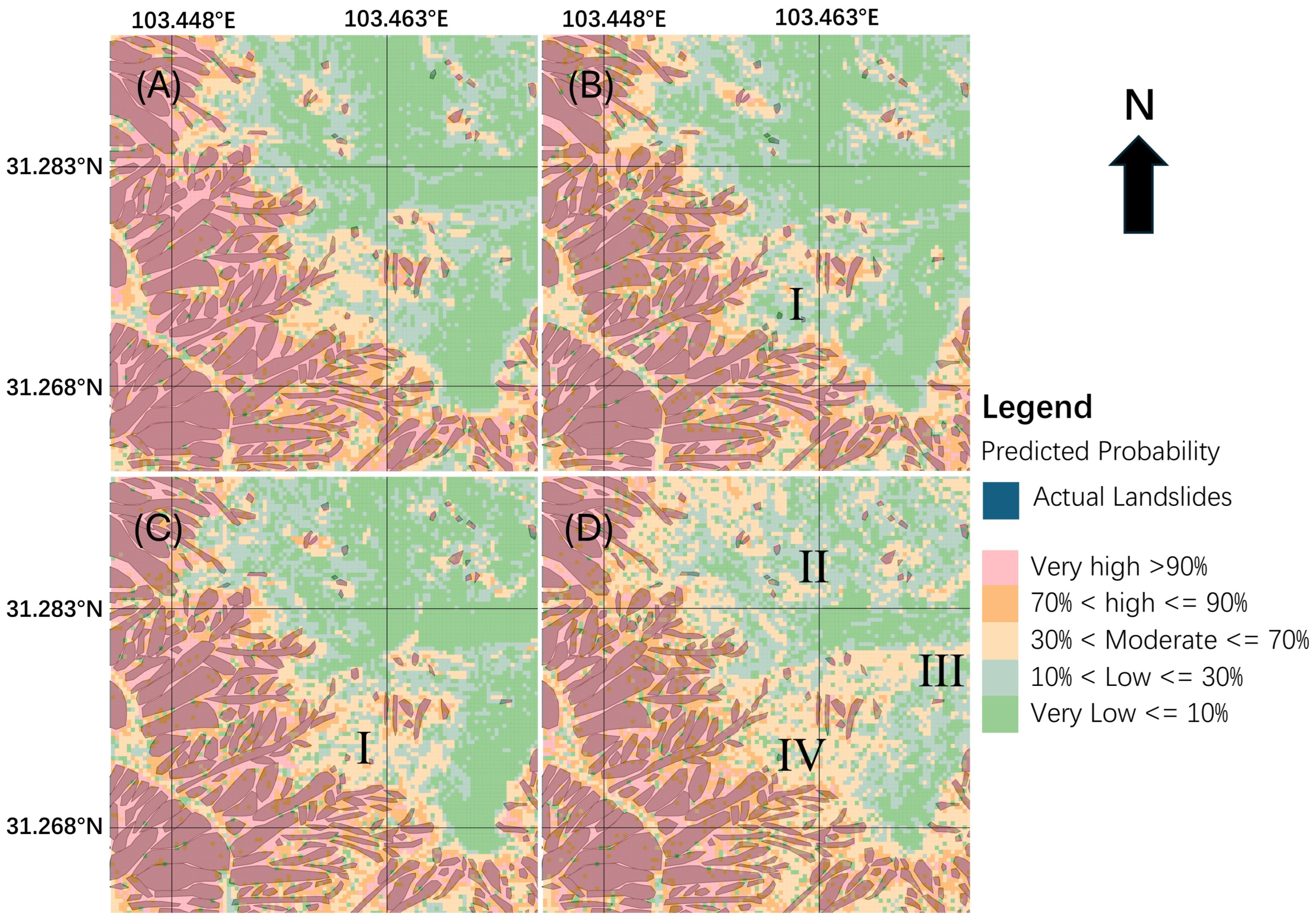
Figure 5.
Comparison of susceptibility maps. The subplots (A–D) are obtained from ERT-A, ERT-B, ERT-C, and ERT-D, respectively. These subplots indicate the various landslide risk locations by using different factors. The various small colored squares represent the different locations of very low to very high susceptibility, and the transition from the landslide area to the non-landslide area is apparent from the change in color of the different small squares. The regions around the Roman numerals in the Figure will be discussed in the text.
Figure 5A–D depict the susceptibility results obtained from ERT-A, ERT-B, ERT-C, and ERT-D, respectively. These maps are divided into five categories based on the predicted landslide probabilities, ranging from 0 to 100%. The categories include Very low (0–10%), Low (10–30%), Moderate (30–70%), High (70–90%), and Very high (over 90%). Utilizing machine learning predictions, each point on the map is assigned to one of these categories. The red areas indicate the highest landslide risk, while the dark green areas represent locations with the lowest risk. The differences between the actual and predicted landslide areas are relatively small in Figure 5C. Notably, Figure 5B, utilizing ERT-B’s input factors, performs better in Region I than in Figure 5C. Conversely, Figure 5D, incorporating non-seismic factors, demonstrates a less accurate assessment of landslides in Regions II, III, and IV, compared to Figure 5A–C.
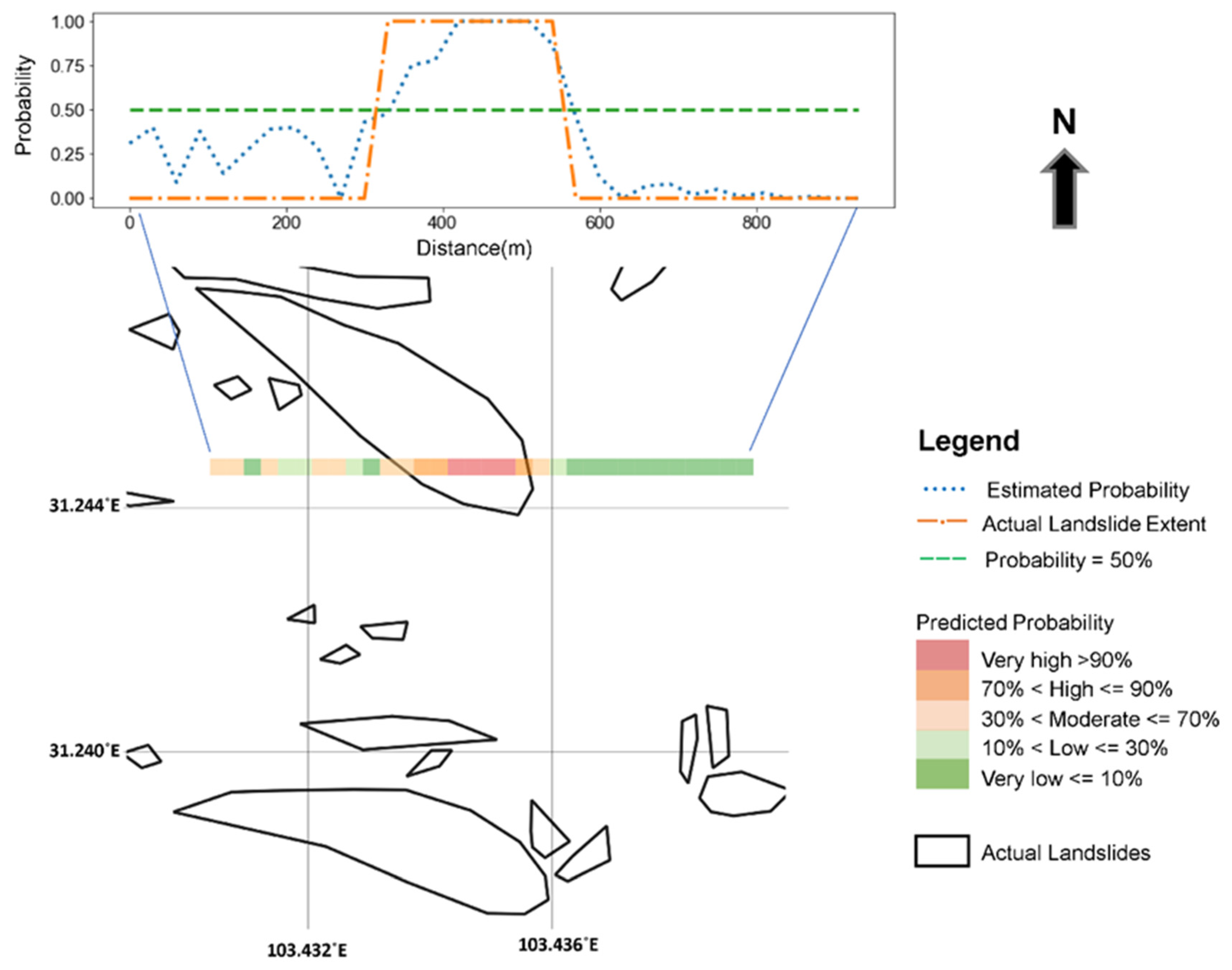
The details of co-seismic landslide estimation and susceptibility mapping are depicted in Figure 6. The figure illustrates the prediction of landslides along a line segment and compares it to the actual landslide area. The small colored squares represent the predicted results from ERT-B, corresponding to the probability line indicated by the blue dashed line in the diagram above. The predicted result, represented by the blue line, provides a reliable representation of the actual landslide area depicted in orange. It is important to note that, in the vicinity of the area with a 50% probability of prediction, indicated by the green dotted line, the predicted results exhibit slight deviations from the actual landslide area. These errors primarily arise from the limitations of the prediction’s resolution, which is set at 30 m.
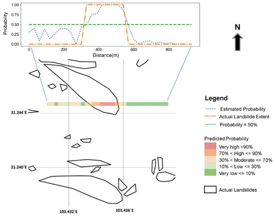
Figure 6.
An example of landslide prediction in a line segment. The line diagram above shows the prediction result (the blue dashed line) and the actual landslide extent (the orange dashed line). The prediction result (the blue dashed line) corresponds to the small colored squares in the plan view below. The colors indicate the estimated probabilities.
The above discussion highlights the significant influence of seismic dynamic parameters on machine learning-based earthquake-induced landslide prediction. It was observed that utilizing distances and azimuths from the epicenter to sites as input factors in machine learning models yields better evaluation results than Peak Ground Accelerations (PGAs). This finding supports the notion that seismic energy is crucial in triggering seismic landslides. The complex geological conditions, surface structure, and various other factors contribute to the non-uniform propagation of seismic energy to the surface. Consequently, certain azimuths experience significantly more damage than others [47]. As a result, distance and azimuth from the epicenter to the site cannot be treated merely as co-ordinates, instead, they are essential seismodynamic parameters involved in the physical process of earthquake-induced landslides. Due to the difficulty of obtaining accurate and realistic large-scale PGAs, using distance and azimuth to replace PGAs to predict landslides is a more practical approach. The conclusions of this study can be used in assessing earthquake-induced disasters predicted by machine learning, such as earthquake-induced landslides or earthquake-induced economic losses.
We have used the co-seismic landslides of the 2008 Wenchuan earthquake as a machine-learning training set. In future studies, machine learning needs should be transferred to consider other earthquakes’ characteristics and co-seismic landslides’ factors when predicting co-seismic landslides in another region. The accuracy of predicting the Wenchuan earthquake landslides in this study using machine learning is 90.2% (Table 3), and further improvement may require measures such as optimizing the model and changing the sampling of inputs. Another way to obtain the accurate ground shaking distribution is the physics-based numerical simulation [48,49,50], which requires large-scale computing and means that the hazard study of earthquakes needs subsequent work.
5. Conclusions
PGAs are closely related to the distance and azimuth of the seismogenic fault. Due to the difficulty of obtaining accurate and realistic large-scale PGAs, this study used the co-seismic landslide records of the 2008 Wenchuan earthquake to train a machine learning model. It presents an alternative approach to assessing the spatial distribution of co-seismic landslides by utilizing distances and azimuths from the epicenter to sites as seismodynamic parameters instead of PGA. The results indicate that these factors effectively predict the spatial distribution of co-seismic landslides. The derived landslide susceptibility map accurately captures the spatial characteristics of landslide and non-landslide areas based on the distance and azimuth from the epicenter to the site. In addition, the authority can apply the conclusion of this study to near-real-time co-seismic landslide prediction. The model using distance and azimuth from the epicenter to the site simplifies the steps, improves the prediction efficiency, and reduces the data processing cost compared to the model relying on PGA. In real emergency rescue scenarios, the conclusions of this study can be used to more conveniently and quickly investigate the range affected by co-seismic landslides without first calculating the PGA. This conclusion will also help society reach the goal of long-lasting, safe, and sustainable development on a regional and global scale.
However, it is essential to acknowledge the limited understanding of the physical processes involved in landslide occurrence, which hampers the interpretation of machine learning methods in landslide prediction. Better seismodynamic factors exist beyond those investigated in this study that could improve co-seismic landslide prediction. The limitation of this study is the need for validation of co-seismic landslides in other parts of the globe. Future work should apply the findings of this study to other areas where co-seismic landslides occur to explore the applicability of this study more broadly.
Author Contributions
Y.S. completed the research and wrote the paper; Z.Z. designed the research and performed the analysis; C.X. guided the use of the software; Y.F. helped revise the article. All authors have read and agreed to the published version of the manuscript.
Funding
This work is supported by the National Natural Science Foundation of China (grant No. 42074054), Guangdong Provincial Key Laboratory of Geophysical High-Resolution Imaging Technology (2022B1212010002), Shenzhen Science and Technology Program (KQTD20170810111725321), and High Level Special Funds (G03050K001).
Institutional Review Board Statement
Not applicable.
Informed Consent Statement
Not applicable.
Data Availability Statement
The data consulted for this article can be found on the following website: (1) landslide inventories in this study provided by the USGS, available at https://www.sciencebase.gov/catalog/item/586d824ce4b0f5ce109fc9a6 (accessed on 26 January 2023); (2) ASTER Global Digital Elevation Model V003 provided the DEM data by NASA EARTHDATA available at Earthdata Search|Earthdata Search (nasa.gov) (access on 20 October 2022); (3) the waterline provided by OpenStreetMap; (4) the faults information provided by the Data Sharing Infrastructure of the National Earthquake Data Center (http://data.earthquake.cn, accessed on 23 January 2023); (5) the information on soil, lithology, and landform provided by the program of the Global Assessment of Land Degradation (GLADA) [51]; (6) peak ground acceleration (PGA) provided by USGS available at https://earthquake.usgs.gov/earthquakes/eventpage/usp000g650/shakemap/pga (accessed on 23 January 2023); (7) slope, aspect, TRI, distance to the waterline, and faults calculated by the Open Source Geographic Information System Quantum GIS (QGis); (8) the distance to and from the epicenter to the site calculated by Python; (9) Figure 2 was created using Generic Mapping Tools; (10) Figure 4, Figure 5 and Figure 6 were generated using QGis and Python.
Acknowledgments
The authors thank Danhua Xin for technical assistance with GIS software (QGIS 3.22.11) and Arnaud Nicolas Mignan for suggestions for article revision. The authors acknowledge the data support from the China Earthquake Networks Center, National Earthquake Data Center (http://data.earthquake.cn, accessed on 23 January 2023).
Conflicts of Interest
The authors declare that the research was conducted in the absence of any commercial or financial relationships that could be construed as a potential conflict of interest.
References
- Dai, F.C.; Lee, C.F.; Ngai, Y.Y. Landslide risk assessment and management: An overview. Eng. Geol. 2002, 64, 65–87. [Google Scholar] [CrossRef]
- Hermanns, R.L. Landslide. In Encyclopedia of Engineering Geology; Bobrowsky, P.T., Marker, B., Eds.; Springer International Publishing: Cham, Switzerland, 2018; pp. 579–580. [Google Scholar] [CrossRef]
- Malamud, B.D.; Turcotte, D.L.; Guzzetti, F.; Reichenbach, P. Landslide inventories and their statistical properties. Earth Surf. Process. Landf. 2004, 29, 687–711. [Google Scholar] [CrossRef]
- Dai, F.C.; Lee, C.F.; Deng, J.H.; Tham, L.G. The 1786 earthquake-triggered landslide dam and subsequent dam-break flood on the Dadu River, southwestern China. Geomorphology 2005, 65, 205–221. [Google Scholar] [CrossRef]
- Zhou, J.-w.; Cui, P.; Fang, H. Dynamic process analysis for the formation of Yangjiagou landslide-dammed lake triggered by the Wenchuan earthquake, China. Landslides 2013, 10, 331–342. [Google Scholar] [CrossRef]
- Keefer, D.K.; Larsen, M.C. Assessing Landslide Hazards. Science 2007, 316, 1136–1138. [Google Scholar] [CrossRef]
- Gorum, T.; Fan, X.; van Westen, C.J.; Huang, R.Q.; Xu, Q.; Tang, C.; Wang, G. Distribution pattern of earthquake-induced landslides triggered by the 12 May 2008 Wenchuan earthquake. Geomorphology 2011, 133, 152–167. [Google Scholar] [CrossRef]
- Hungr, O.; McDougall, S. Two numerical models for landslide dynamic analysis. Comput. Geosci. 2009, 35, 978–992. [Google Scholar] [CrossRef]
- Carrara, A.; Cardinali, M.; Detti, R.; Guzzetti, F.; Pasqui, V.; Reichenbach, P. GIS techniques and statistical models in evaluating landslide hazard. Earth Surf. Process. Landf. 1991, 16, 427–445. [Google Scholar] [CrossRef]
- Lee, C.-T.; Huang, C.-C.; Lee, J.-F.; Pan, K.-L.; Lin, M.-L.; Dong, J.-J. Statistical approach to earthquake-induced landslide susceptibility. Eng. Geol. 2008, 100, 43–58. [Google Scholar] [CrossRef]
- Guzzetti, F.; Carrara, A.; Cardinali, M.; Reichenbach, P. Landslide hazard evaluation: A review of current techniques and their application in a multi-scale study, Central Italy. Geomorphology 1999, 31, 181–216. [Google Scholar] [CrossRef]
- Xu, C.; Xu, X.W.; Dai, F.C.; Saraf, A.K. Comparison of different models for susceptibility mapping of earthquake triggered landslides related with the 2008 Wenchuan earthquake in China. Comput. Geosci. 2012, 46, 317–329. (In English) [Google Scholar] [CrossRef]
- Tien Bui, D.; Tuan, T.A.; Klempe, H.; Pradhan, B.; Revhaug, I. Spatial prediction models for shallow landslide hazards: A comparative assessment of the efficacy of support vector machines, artificial neural networks, kernel logistic regression, and logistic model tree. Landslides 2016, 13, 361–378. [Google Scholar] [CrossRef]
- Dou, J.; Yunus, A.P.; Tien Bui, D.; Merghadi, A.; Sahana, M.; Zhu, Z.; Chen, C.-W.; Khosravi, K.; Yang, Y.; Pham, B.T. Assessment of advanced random forest and decision tree algorithms for modeling rainfall-induced landslide susceptibility in the Izu-Oshima Volcanic Island, Japan. Sci. Total Environ. 2019, 662, 332–346. [Google Scholar] [CrossRef] [PubMed]
- Merghadi, A.; Yunus, A.P.; Dou, J.; Whiteley, J.; ThaiPham, B.; Bui, D.T.; Avtar, R.; Abderrahmane, B. Machine learning methods for landslide susceptibility studies: A comparative overview of algorithm performance. Earth Sci. Rev. 2020, 207, 103225. [Google Scholar] [CrossRef]
- Fan, X.; Fang, C.; Dai, L.; Wang, X.; Luo, Y.; Wei, T.; Wang, Y. Near real time prediction of spatial distribution probability of earthquake-induced landslides—Take the lushan earthquake on June 1, 2022 as an example. J. Eng. Geol. 2022, 30, 729–739. [Google Scholar] [CrossRef]
- Liu, R.; Yang, X.; Xu, C.; Wei, L.S.; Zeng, X.Q. Comparative Study of Convolutional Neural Network and Conventional Machine Learning Methods for Landslide Susceptibility Mapping. Remote Sens. 2022, 14, 321. [Google Scholar] [CrossRef]
- Sun, X.H.; Yu, C.L.; Li, Y.R.; Rene, N.N. Susceptibility Mapping of Typical Geological Hazards in Helong City Affected by Volcanic Activity of Changbai Mountain, Northeastern China. Isprs Int. J. Geo-Inf. 2022, 11, 344. [Google Scholar] [CrossRef]
- Wang, X.; Wang, X.; Zhang, X.; Wang, L.; Guo, H.; Li, D. Near real-time spatial prediction of earthquake-induced landslides: A novel interpretable self-supervised learning method. Int. J. Digit. Earth 2023, 16, 1885–1906. [Google Scholar] [CrossRef]
- Su, L.Y.; Gui, Y.N.; Xu, L.; Ming, D.P. Rain-Induced Landslide Hazard Assessment Using Inception Model and Interpretability Method—A Case Study of Zayu County, Tibet. Appl. Sci. Basel 2024, 14, 5324. [Google Scholar] [CrossRef]
- Dai, F.C.; Xu, C.; Yao, X.; Xu, L.; Tu, X.B.; Gong, Q.M. Spatial distribution of landslides triggered by the 2008 Ms 8.0 Wenchuan earthquake, China. J. Asian Earth Sci. 2011, 40, 883–895. [Google Scholar] [CrossRef]
- Dai, L.; Fan, X.; Wang, X.; Fang, C.; Zou, C.; Tang, X.; Wei, Z.; Xia, M.; Wang, D.; Xu, Q. Coseismic landslides triggered by the 2022 Luding Ms6.8 earthquake, China. Landslides 2023, 20, 1277–1292. [Google Scholar] [CrossRef]
- Fan, X.; Scaringi, G.; Korup, O.; West, A.J.; van Westen, C.J.; Tanyas, H.; Hovius, N.; Hales, T.C.; Jibson, R.W.; Allstadt, K.E.; et al. Earthquake-Induced Chains of Geologic Hazards: Patterns, Mechanisms, and Impacts. Rev. Geophys. 2019, 57, 421–503. [Google Scholar] [CrossRef]
- Fan, X.; Yunus, A.P.; Scaringi, G.; Catani, F.; Siva Subramanian, S.; Xu, Q.; Huang, R. Rapidly Evolving Controls of Landslides After a Strong Earthquake and Implications for Hazard Assessments. Geophys. Res. Lett. 2021, 48, e2020GL090509. [Google Scholar] [CrossRef]
- Xu, C.; Xu, X.; Shyu, J.B.H.; Gao, M.; Tan, X.; Ran, Y.; Zheng, W. Landslides triggered by the 20 April 2013 Lushan, China, Mw 6.6 earthquake from field investigations and preliminary analyses. Landslides 2015, 12, 365–385. [Google Scholar] [CrossRef]
- Xu, C.; Xu, X.; Wu, X.; Dai, F.; Yao, X.; Yao, Q. Detailed catalog of landslides triggered by the 2008 wenchuan earthquake and statistical analyses of their spatial distribution. J. Eng. Geol. 2013, 21, 25–44. [Google Scholar]
- Xu, C.; Xu, X.; Yao, X.; Dai, F. Three (nearly) complete inventories of landslides triggered by the May 12, 2008 Wenchuan Mw 7.9 earthquake of China and their spatial distribution statistical analysis. Landslides 2014, 11, 441–461. [Google Scholar] [CrossRef]
- Xu, C.; Xu, X.; Yu, G. Landslides triggered by slipping-fault-generated earthquake on a plateau: An example of the 14 April 2010, Ms 7.1, Yushu, China earthquake. Landslides 2013, 10, 421–431. [Google Scholar] [CrossRef]
- Xu, C.; Xu, X.W.; Lee, Y.H.; Tan, X.B.; Yu, G.H.; Dai, F.C. The 2010 Yushu earthquake triggered landslide hazard mapping using GIS and weight of evidence modeling. Environ. Earth Sci. 2012, 66, 1603–1616. [Google Scholar] [CrossRef]
- Marc, O.; Meunier, P.; Hovius, N. Prediction of the area affected by earthquake-induced landsliding based on seismological parameters. Nat. Hazards Earth Syst. Sci. 2017, 17, 1159–1175. [Google Scholar] [CrossRef]
- Meunier, P.; Hovius, N.; Haines, A.J. Regional patterns of earthquake-triggered landslides and their relation to ground motion. Geophys. Res. Lett. 2007, 34, L20408. [Google Scholar] [CrossRef]
- Xin, D.; Zhang, Z. On the Comparison of Seismic Ground Motion Simulated by Physics-Based Dynamic Rupture and Predicted by Empirical Attenuation Equations. Bull. Seismol. Soc. Am. 2021, 111, 2595–2616. [Google Scholar] [CrossRef]
- Aki, K.; Richards, P.G. Quantitative Seismology. In Elastic Waves from a Point Dislocation Source, 2nd ed.; Ellis, J., Ed.; University Science Books: Herndon, VA, USA, 2002; pp. 63–117. [Google Scholar]
- Boore, D.M.; Atkinson, G.M. Ground-Motion Prediction Equations for the Average Horizontal Component of PGA, PGV, and 5%-Damped PSA at Spectral Periods between 0.01 s and 10.0 s. Earthq. Spectra 2008, 24, 99–138. [Google Scholar] [CrossRef]
- Campbell, K.W.; Bozorgnia, Y. NGA Ground Motion Model for the Geometric Mean Horizontal Component of PGA, PGV, PGD and 5% Damped Linear Elastic Response Spectra for Periods Ranging from 0.01 to 10 s. Earthq. Spectra 2008, 24, 139–171. [Google Scholar] [CrossRef]
- Li, X.; Zhou, Z.; Yu, H.; Wen, R.; Lu, D.; Huang, M.; Zhou, Y.; Cu, J. Strong motion observations and recordings from the great Wenchuan Earthquake. Earthq. Eng. Eng. Vib. 2008, 7, 235–246. [Google Scholar] [CrossRef]
- Zhang, W.; Shen, Y.; Chen, X. Numerical simulation of strong ground motion for the Ms8.0 Wenchuan earthquake of 12 May 2008. Sci. China Ser. D Earth Sci. 2008, 51, 1673–1682. [Google Scholar] [CrossRef]
- Fan, X.; Scaringi, G.; Xu, Q.; Zhan, W.; Dai, L.; Li, Y.; Pei, X.; Yang, Q.; Huang, R. Coseismic landslides triggered by the 8th August 2017 Ms 7.0 Jiuzhaigou earthquake (Sichuan, China): Factors controlling their spatial distribution and implications for the seismogenic blind fault identification. Landslides 2018, 15, 967–983. [Google Scholar] [CrossRef]
- Sokolova, M.; Lapalme, G. A systematic analysis of performance measures for classification tasks. Inf. Process. Manag. 2009, 45, 427–437. [Google Scholar] [CrossRef]
- Fawcett, T. An introduction to ROC analysis. Pattern Recognit. Lett. 2006, 27, 861–874. [Google Scholar] [CrossRef]
- Bradley, A.P. The use of the area under the ROC curve in the evaluation of machine learning algorithms. Pattern Recognit. 1997, 30, 1145–1159. [Google Scholar] [CrossRef]
- Geurts, P.; Ernst, D.; Wehenkel, L. Extremely randomized trees. Mach. Learn. 2006, 63, 3–42. [Google Scholar] [CrossRef]
- Wei, J.; Li, Z.; Cribb, M.; Huang, W.; Xue, W.; Sun, L.; Guo, J.; Peng, Y.; Li, J.; Lyapustin, A.; et al. Improved 1 km resolution PM2.5 estimates across China using enhanced space–time extremely randomized trees. Atmos. Chem. Phys. 2020, 20, 3273–3289. [Google Scholar] [CrossRef]
- Xu, Z.Q.; Ji, S.C.; Li, H.B.; Hou, L.W.; Fu, X.F.; Cai, Z.H. Uplift of the Longmen Shan range and the Wenchuan earthquake. Episodes 2008, 31, 291–301. [Google Scholar] [CrossRef]
- Pei-Zhen, Z.; XiWei, X.U.; XueZe, W.E.N.; YongKang, R.A.N. Slip rates and recurrence intervals of the Longmen Shan active fault zone, and tectonic implications for the mechanism of the May 12 Wenchuan earthquake, 2008, Sichuan, China. Chin. J. Geophys. 2008, 51, 1066–1073. [Google Scholar]
- Xu, X.; Wen, X.; Yu, G.; Chen, G.; Klinger, Y.; Hubbard, J.; Shaw, J. Coseismic reverse- and oblique-slip surface faulting generated by the 2008 Mw 7.9 Wenchuan earthquake, China. Geology 2009, 37, 515–518. [Google Scholar] [CrossRef]
- Li, Y.; Zhang, Z.; Wang, W.; Feng, X. Rapid Estimation of Earthquake Fatalities in Mainland China Based on Physical Simulation and Empirical Statistics—A Case Study of the 2021 Yangbi Earthquake. Int. J. Environ. Res. Public Health 2022, 19, 6820. [Google Scholar] [CrossRef]
- Pelties, C.; de la Puente, J.; Ampuero, J.-P.; Brietzke, G.B.; Käser, M. Three-dimensional dynamic rupture simulation with a high-order discontinuous Galerkin method on unstructured tetrahedral meshes. J. Geophys. Res. Solid Earth 2012, 117, B02309. [Google Scholar] [CrossRef]
- Zhang, W.; Liu, Y.; Chen, X. A Mixed-Flux-Based Nodal Discontinuous Galerkin Method for 3D Dynamic Rupture Modeling. J. Geophys. Res. Solid Earth 2023, 128, e2022JB025817. [Google Scholar] [CrossRef]
- Zhang, Z.; Zhang, W.; Chen, X. Three-dimensional curved grid finite-difference modelling for non-planar rupture dynamics. Geophys. J. Int. 2014, 199, 860–879. [Google Scholar] [CrossRef]
- Dijkshoorn, J.; van Engelen, V.; Huting, J. Soil and Landform Properties for LADA Partner Countries (Argentina, China, Cuba, Senegal and The Gambia, South Africa and Tunisia); ISRIC Report 2008/06 and GLADA Report 2008/03; ISRIC—World Soil Information and FAO: Wageningen, The Netherlands, 2008; Available online: https://www.isric.org/sites/default/files/isric_report_2008_06.pdf (accessed on 23 February 2023).


Disclaimer/Publisher’s Note: The statements, opinions and data contained in all publications are solely those of the individual author(s) and contributor(s) and not of MDPI and/or the editor(s). MDPI and/or the editor(s) disclaim responsibility for any injury to people or property resulting from any ideas, methods, instructions or products referred to in the content. |
© 2024 by the authors. Licensee MDPI, Basel, Switzerland. This article is an open access article distributed under the terms and conditions of the Creative Commons Attribution (CC BY) license (https://creativecommons.org/licenses/by/4.0/).