Abstract
The seasonal fluctuation of river depths is a critical factor in designing cargo capacity for river convoys and logistics processes used for grain transportation in northern Brazil. Water level variations directly impact the load capacities of pusher convoys navigating the Amazon rivers. This paper presents a machine learning model based on a multilayer perceptron artificial neural network developed with the aim of estimating the cargo capacities of river convoys one year in advance, which is essential for determining load capacities during dry periods. The prediction model was applied to the Tapajós River in the Amazon Basin, Brazil, where grain transportation is significant and relies on inland waterways. Navigability conditions were evaluated in terms of depth and geometric parameters. The results of this case study were satisfactory, validating the computational tool and enabling the assessment of capacity losses during dry periods and the identification of navigation bottlenecks. The main contributions of this work include optimizing river logistics, reducing costs, minimizing environmental impacts, and promoting the sustainable management of water resources in the Amazon. Conclusions drawn from the study indicate that the developed model is highly effective, with an R2 of 0.954 and RMSE of 0.095, demonstrating its potential to significantly enhance river convoy operations and support sustainable development in the region.
1. Introduction
Inland waterways play a crucial role in the logistics chain [1,2], as they allow for low-cost transportation of large volumes of goods, resulting in a significant reduction of the environmental impacts and a substantial increase in logistical efficiency [3,4,5]. The management and parameterization of inland waterways enable the creation of a transportation infrastructure capable of fostering the sustainable development of remote coastal areas and supporting the extraction as well as transportation of resources and manufactured products, thereby justifying their importance for sustainable development [1,6,7].
When analyzing the Amazonian scenario, Brazilian foreign trade has increased in recent decades. This has also led to a growing utilization of the waterways for the transportation of the produced goods, especially bulk agricultural goods, thus increasing the importance of the port structures responsible for this flow [8]. In terms of cargo transportation via the waterway mode, utilizing port structures leads to significant cost reductions per ton compared to other modes [9,10]. Similarly, there are technical and economic impacts resulting from the structural capacity to handle large quantities of cargo [8]. According to Teixeira et al. [11], although the export potential through port terminals is far from being fully exploited, a significant portion of the cargo volume is being transported via river routes to ports that redirect these goods to the international market, such as the ports that make up the Northern Arc logistics corridors.
The Amazon Basin, with its vast network of rivers, plays a pivotal role in the economic and environmental landscape of northern Brazil. Among the various challenges faced in this region, the seasonal fluctuation of river depths significantly impacts the logistics of grain transportation, which is a critical economic activity in the area. The ability to effectively manage these fluctuations is essential for optimizing cargo capacities and ensuring efficient navigation throughout the year.
Seasonal variations in river depth can have profound implications for the capacity and safety of river convoys. During the dry season, reduced water levels can constrain the navigability of waterways, leading to decreased load capacities and increased transportation costs. Conversely, during the wet season, higher water levels may present their own set of challenges, including potential overloading and increased risk of navigation hazards. Consequently, accurate prediction and management of these fluctuations are crucial for maintaining operational efficiency and cost-effectiveness in river transport.
In this context, the development of advanced predictive tools is essential. Machine learning, with its capacity for processing large datasets and uncovering complex patterns, offers a promising approach for forecasting seasonal depth variations and optimizing river convoy operations. This paper presents a machine learning model based on a multilayer perceptron (MLP) artificial neural network designed to predict cargo capacities of river convoys in advance, specifically focusing on the Tapajós River in the Amazon Basin.
The importance of the research aim and novelties lies in its potential to significantly contribute to sustainable development by providing a comprehensive method to anticipate and manage seasonal depth changes. This capability ensures that the transportation of goods, particularly in the ecologically sensitive Amazon Basin, is conducted in a manner that minimizes environmental impact [12]. By optimizing cargo capacities for river convoys through advanced machine learning techniques, this approach supports sustainable economic growth and infrastructure development while protecting natural resources [13,14,15]. Focusing on the sustainable management of inland waterways, this research addresses immediate logistical challenges and establishes a framework for long-term environmental stewardship and socio-economic development [16].
The present study aims to evaluate the vessel loading conditions by developing a machine learning-based model for water level prediction using multilayer perceptron artificial neural networks with the backpropagation algorithm. The model predicts available depths in a specific waterway, allowing for the subsequent calculation of Under-Keel Clearance (UKC) values. This enables the determination of vessel drafts and load capacities for safe and economically viable navigation. The model was applied in the Tapajós River Basin in the Amazon region, involving the sizing, modeling, and hydrostatic analysis of a typical 5 × 5 pushboat convoy consisting of 25 standard Mississippi barges. The geometric conditions of the navigable waterway were evaluated in terms of depth and geometric parameters, utilizing a digital elevation model to assess the impacts of seasonal watercourse fluctuations on cargo capacity and to verify the constraints generated during low-water periods, including available depth, width, and total convoy load capacity.
2. Literature Review
2.1. Importance of Inland Waterway Transportation
Inland waterways play a crucial role in the logistics chain [1,2], facilitating low-cost transportation of large volumes of goods while significantly reducing environmental impact and increasing logistical efficiency [3,4,5]. The management of these waterways allows for the development of a natural transportation infrastructure that supports the development of remote coastal areas through the extraction and transportation of resources and manufactured products, thus underscoring their importance [1,6].
In the context of Amazon, the growing Brazilian foreign trade over recent decades has highlighted the increasing use of the waterway mode for transporting produced goods, especially bulk agricultural goods, thereby emphasizing the importance of the port infrastructure responsible for this distribution [17]. Utilizing waterway transport with port facilities results in significant reductions in costs per ton compared to other transport modes [9,10,18,19]. Similarly, there are noticeable technical and economic impacts of the structural capacity required for handling large quantities of cargo [8,13,20,21].
2.2. Navigation Challenges
Despite the acknowledged importance of waterway transport, the safety of navigation on rivers and lakes has not developed proportionally to the increased demand for this mode due to various infrastructural, climatic, and hydrological challenges [22,23,24]. Natural factors such as tidal phenomena, river geomorphology, sedimentation and erosion issues, and seasonal water level variations [17,23,25,26,27,28] significantly contribute to these challenges, impeding the full utilization of inland waterways.
2.3. Seasonal Variability of Water Levels
Seasonal variability in water depths is a critical factor affecting the navigability and operational efficiency of vessels. Floods and droughts lead to fluctuations in water depth and draft, thereby impacting vessel carrying capacities [26]. During low-water levels, vessels must reduce their cargo volumes by decreasing draft values, which can result in increased transportation costs per ton. Therefore, analyzing navigability conditions and hydrological processes is fundamental for an efficient management of inland waterways [29,30].
In this context, it is evident that inland waterways are vulnerable to climate change, as river navigation depends heavily on water levels [31]. Droughts can severely impair inland navigation services by reducing water levels to non-navigable conditions or forcing operators to decrease vessel loads [32].
In the context of previous research, Vidyalashmi et al. [33] analyzed a water level forecast model for the Chikugo River estuary in Japan using nonlinear autoregressive with exogenous inputs (NARX Model), considering previous water level, river discharge, and salinity. Liu and Huang [34] developed a deep learning computer vision for water level monitoring and management in river systems using both the traditional continuous image subtraction (CIS) approach and a SegNet neural network. Li et al. [35] developed a combined hydrodynamic model and deep learning method to predict water level in ungauged rivers, which was tested in a section of the Yangtze River. The results showed that the hydrodynamic model can provide the foundation for water level prediction in ungauged sites. Wang et al. [36] developed a model for assessment of the joint impact of rainfall and river water level on urban flooding in Wuhan City, China.
2.4. Influence of Precipitation on Hydrological Analyses
Precipitation is a key component of the hydrological cycle, necessary for monitoring and understanding water balances, which in turn inform hydrological modeling and climate change predictions [37]. Its significance in assessing and managing risks in river basins is crucial [38].
Supporting this, the literature indicates that precipitation is among the vital components of the water cycle, playing a fundamental role in decision-making related to navigation planning, agricultural production, food security, water resource management, and hydropower generation [39,40,41]. For instance, precipitation is a primary variable in evaluating extreme climate variations, such as droughts [42,43,44].
2.5. Use of Neural Networks in Hydrology
Seo et al. [45] predicted water levels using artificial intelligence techniques. Scheepers et al. evaluated the impact of climate variables influencing navigation on the Mackenzie River from the perspective of water level reduction effects. Le Carrer et al. [46] optimized vessel loading using stochastic techniques to assess water level fluctuations. Li et al. [47] developed and validated an artificial neural network model based on random forests (RF) to assess the hydrological conditions in water courses in China. Khan et al. [48] used RNA models to predict flow rates and water levels in the Ramganga River, India. Phan and Nguyen [49] analyzed the Red River in Asia from a stochastic perspective using statistical models to forecast water levels. In the Amazon Basin, Figueiredo and Blanco [50] used ARIMA stochastic models to forecast flow rates and water levels in the Tapajós River. Barbosa et al. [51] developed a computational tool for designing navigation channels to verify navigability conditions based on the seasonal behavior of the Tapajós River.
Garcia et al. [52] applied a random forest algorithm on the Cagayan River in the Philippines to predict water levels and improve navigability conditions of inland waterways. Whang et al. [53] utilized feed-forward neural networks (FFNN) and deep learning (DL) to forecast monthly water column height in Polish lake regions. Li et al. [54] applied a hybrid artificial intelligence-based method to obtain water level values in China.
3. Materials and Methods
The research was based on two intrinsic objectives: predicting the load capacity of pushboat convoys based on seasonal variability of depth and predicting the geometric parameters required for the layout of inland waterway navigation channels. The model was applied by modeling the load capacity of fluvial convoys involved in grain transportation on the Tapajós River in the Amazon, Brazil. Table 1 provides a general illustration of the methodological flow chart subdivided into various steps.

Table 1.
Methodological steps.
3.1. Water Level Forecast
The adopted machine learning method aimed to obtain and define a stochastic model capable of correlating input data, which described the behavior of the phenomenon, with output data, which represented the phenomenon itself, to simulate deductive behavior. Given their deductive capacity, neural networks can find correlations between linear and nonlinear variables, as well as correlations involving integration and differentiation of the input data, without any modifications to the data. However, prior analysis is necessary to ensure the proper formatting of input information, facilitating model convergence and delivering better results.
The correlation process within the adopted machine learning model, specifically the multilayer perceptron (MLP) artificial neural network, is designed to establish relationships between input variables (historical water level data and environmental factors) and output predictions (future water levels). Here is a more detailed explanation of how the model achieves this correlation:
- i.
- Input–Output mapping: The model takes historical water level data (input) as well as lagged and differentiated variables to better capture the cyclical nature of water levels. The historical data serve as a foundation for understanding patterns in river depth changes over time. By using these inputs, the model attempts to map them to the corresponding output, which is the predicted water level for future periods.
- ii.
- Layered neural network structure: The MLP consists of multiple layers of neurons (as mentioned, two intermediate layers in the MLP16 model). Each layer processes input data to extract features and patterns. The neurons within each layer are connected by weights, which represent the strength of the correlation between input data and output predictions. During training, these weights are adjusted to reduce the error between the predicted and actual water levels.
- iii.
- Correlation through training: The model is trained using backpropagation, where errors from the output layer (the difference between predicted and actual water levels) are propagated back through the network. This process updates the weights between the neurons, allowing the model to gradually learn the correlations between the input data and the correct output (future water levels). The goal is to minimize prediction errors, facilitating better correlation between the input historical data and the predicted output.
- iv.
- Normalization and lagging for correlation: To improve the model’s ability to correlate data, the input variables are normalized (using techniques like MinMaxScaler) and lagged. Normalization ensures that the input data are scaled consistently, preventing the model from being biased toward variables with larger magnitudes. Lagging allows the model to capture temporal dependencies by considering water level data from previous time periods as input, thus better correlating the cyclic seasonal nature of water levels with the output predictions.
- v.
- Hidden layers and nonlinear relationships: The hidden layers in the MLP model allowed the network to capture both linear and nonlinear correlations between the input and output. This was crucial for water level prediction, as the relationship between environmental factors (such as precipitation, river flow, and seasonal changes) and water levels is often nonlinear. The neurons in these hidden layers applied activation functions (e.g., ReLU) to transform the input data and establish the correlation between complex variables.
- vi.
- Model convergence: Convergence in the model is achieved when the correlation between input data and predicted output stabilizes, meaning that further adjustments to the weights do not significantly reduce prediction errors. The Adam optimizer is used during training to dynamically adjust the learning rate, helping the model converge efficiently by finding the optimal weight values that correlate input patterns with accurate predictions.
In summary, the model correlates historical water level data with future predictions through a series of processes, including layered neuron connections, weight adjustments, normalization, lagging, and nonlinear feature extraction. These elements work together to ensure that the model can accurately predict water levels by identifying complex patterns and relationships in the input data.
In the case at hand, the model utilized input data like output values under different conditions. Lagging and/or differentiation of the inputs were performed to provide a more adaptable and trainable model, requiring less computational effort while ensuring greater reliability. Thus, the neural network model not only associates distinct variables but also self correlates to the same types of data, exhibiting the behavior of iterative functions. Figure 1 illustrates the structure of ANN models, specifically the perceptron type, highlighting the input and output data as well as the network layers.
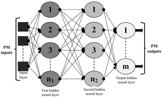
Figure 1.
Perceptron-type ANN model.
The module for developing the water level prediction model involved designing, structuring, calibrating, validating, and training the multilayer perceptron (MLP) artificial neural network (ANN). The MLP was trained using the backpropagation (BP) training algorithm. The architecture of the neural network is shown in Figure 1.
MLP-type ANNs consist of three primary components: the input layer, which is composed of a set of sensory units; one or more hidden layers; and the output layer (Feng et al. [55]). Based on the methodological framework of the multilayer perceptron (MLP) structure depicted in Figure 2, with a single hidden layer, each neuron in the hidden layer can be calculated using Equation (1) [55,56].
Here represents the i-th input to the network; is the weight of the connection from the input neuron to the hidden neuron ; is the bias of the j-th hidden neuron; and is the activation function of the neuron.
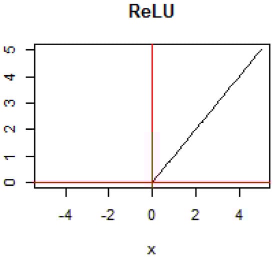
Figure 2.
ReLU activation function for multilayer perceptron neural networks.
For the MLP-type ANN illustrated in Figure 2, each neuron in the output layer is determined using Equation (2), as referenced in Haykin [57].
Here is the weight of the connection from hidden neuron j to output neuron k, is the k-th output of the network, is the bias of the k-th output, and is the activation function of the neuron.
The core equations for an MLP-type network were established, necessitating the selection of the learning algorithm and its mathematical properties. The water level prediction was then executed using an MLP-type neural network with the backpropagation algorithm (MLP-BP).
3.1.1. Definition of Temporal and Variational Correlation
The process of lagging the water level data was developed considering the amount of data available in the historical series. Performing lagging operations implies a loss of available data, not only for the training process but also for model validation. Considering n lags, the amount of lost data becomes 2n, considering that all the preceding and succeeding water level data required for correct filling are not present in the available hydrological cycle sample.
Developing input variables with a varying nature becomes less significant when considering that a temporal correlation will already be performed and that temporal data have a cyclic pattern. Taking this into account, RNNs can capture the varying aspects of the model.
3.1.2. Data Normalization
To reduce redundancy and computational effort while increasing data integrity and performance, the input data were normalized. This practice is employed to prevent the algorithm from being biased towards variables with larger magnitudes. The MaxMinScaler normalization technique was applied, which scales all values received between 0 and 1 using the formulation defined in Equation (3), as referenced in Haykin [57].
Here represents the normalized variable value, is the actual value of the variable, is the minimum value among the analyzed dataset, and is the maximum value among the analyzed dataset.
3.1.3. Parameters Definition
Specific backpropagation algorithms were utilized for the perceptron neural network during the training process [53,55,58]. These algorithms involve optimization methods with parameters defined by variable and constant values that determine the training details. These parameters were defined prior to the start of this stage, including the activation function characteristics and initial learning rate. They are crucial for aiding in weight adaptation within the neural networks. Additionally, other parameters were defined, such as the maximum number of iterations (set to 800) and the tolerance for ending training (set to 104). These parameters are essential for determining the ideal moment to conclude the training process, as they prevent further iterations when significant changes in the obtained errors are not observed.
The neural network inputs’ neurological stimuli and the model composition were mathematically described using an activation function [59,60], typically of a nonlinear nature, which alters the received stimulus value and enables the networks’ high adaptability to various applications. In this regard, the ReLU activation function [61,62] was used, which does not have a unique formulation but is presented in Figure 2.
When using the ReLU activation function, the parameter Alpha is employed, representing a slope of the ReLU function for all values where x < 0. This parameter is important as it helps alleviate the loss of functionality that occurs during training. The backpropagation training model requires that weight adaptation be based on the derivative of the activation function into which the weights are inserted. If the sum of a given neuron reaches 0, the training process for that specific neuron no longer occurs.
3.1.4. Training Process
The solver method used for weight update was the ‘Adam’ method proposed by Kingma and Ba [63]. It involves a training process with gradient descent combined with a momentum factor known as Momentum.
The inputs to the neuron were obtained through a weighted sum with weights that are adjusted during the training process. The weighted sum, along with the neural network, provides a final response representing the output data or another weighted input among others for one or more neurons in the next layer [53,55,64]. Mathematically, the set of expressions describing the behavior of multilayer perceptron neural networks can be defined by Equations (4)–(7), as referenced in Haykin [57].
Here represents the final output function, which is the ReLU function; is the output bias; is an inherent error in the optimization model, which is present in any empirical statistical method; r represents the output function of neuron i in layer h; and presents the weight of neuron i in layer h. The value represents a constant, which is the input value inserted into the neural network.
Regarding the first layer, it does not have activation functions, meaning there is no processing involved. Its sole purpose is to receive the input data and pass it on to the subsequent neurons. The only processing that occurs is the weighting of the inputs, providing an importance level for each variable.
This article applies varied parameters in the training process, primarily through the dynamic adaptation of the learning rate, momentum, and weight adjustments. This ensures that the model can effectively adapt and learn complex patterns in the data, achieving more accurate predictions. The architecture itself (the number of neurons and layers) remains constant, but the parameters that govern learning are varied.
3.1.5. Variable Parameters Definition
The backpropagation algorithm, proposed by David E. Rumelhart, Geoffrey E. Hinton, and Ronald J. Williams, was used as the optimization process for adjusting the synaptic weights. This method aimed to minimize the error derived from the synaptic weights by employing gradient reduction techniques with activation functions. The backpropagation process is defined by Equations (8) and (9), as referenced in Wang et al. [65,66] and Chen et al. [58].
Here represents the training cycle, are the synaptic weights in cycle k, é is the learning rate at cycle , represents the errors in the output layer, is the derivative of the activation function used, represents the inputs in the current layer, and s represents the subsequent layer for which the weight update is being performed.
The functional nature of the models is not only determined by their parameters but also by their architecture. Consequently, multiple models were created to select the best one. Throughout the training process, the layers had randomly generated weights. The acceleration of training and its convergence were achieved by adjusting the learning rate, which could be constant or varied.
The learning rate was defined as a constant value plus a variation given by the momentum factor, as defined by Wang and Sheng [67] and utilized in Nourani [68] and Azad et al. [64]. The weight update was the sum of the change between the current step and the previously calculated weight, multiplied by the learning rate constant μ, and added to the direction correction of the current iteration. Therefore, when the last weight change occurred in a specific direction, the momentum ensured that the next weight change would also be in the same direction. The calculation of the momentum factor is defined by Equation (10), as referenced in Wang and Sheng [67] and utilized in Nourani [68].
Here represents the variation from the current iteration to the next, μ is the learning rate, represents the change in error at cycle k, and (t) represents the current weight variation in the current iteration.
3.1.6. Metrics Definitions
Performance assessment was conducted using widely used metrics in the literature, namely the Coefficient of Determination (R2) and Root Mean Squared Error (RMSE), as utilized in Sahoo et al. [69], Valipour et al. [70], Kumar [71], and Coulibaly et al. [72]. These are defined by Equations (11) and (12), respectively.
Here is the mean of the values in the historical series, represents the predicted value by the model, and represents the actual value.
3.2. Vessel Hydrostatic Modeling
Hydrostatic Properties
Based on the hull modeling using the lines plan and the three-dimensional arrangement, it becomes possible to determine the hydrostatic properties of the designed vessel. These properties are fundamental for understanding the hydrostatic behavior of the vessel in relation to its draught, and they are useful for determining loading plans, onboard weight distribution, and stability studies [73,74,75].
Based on the calculations of the hydrostatic properties, it is possible to calculate the load capacities for a given loading condition. To calculate the load capacities, subtract the displacement value from the lightweight tonnage (LWT). Adland et al. [76] state that the deadweight tonnage (DWT) of a vessel is characterized as the maximum load capacity of the vessel under international regulations. Equation (13) shows how to calculate the load capacity of the vessel for a given draught.
Here is the density of water; is the acceleration due to gravity; represents the area curve of each compartment; and is an infinitesimal longitudinal distance.
3.3. Planialtimetric Conditions
According to [51,77,78], ensuring safe navigation in a given waterway or canal requires defining the minimum geometric characteristics of the watercourse in terms of horizontal dimensions (width of straight and curved stretches) and vertical dimensions (required minimum depths). These geometric variables are dependent on factors related primarily to the design of the vessel, topographic conditions, weather conditions, and hydrological conditions. In this regard, due to the need for defining the geometric characteristics of the study case waterway, the horizontal and vertical conditions were determined based on Figure 3.
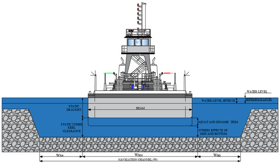
Figure 3.
Geometric parameters of waterways.
3.3.1. Horizontal Dimensions
The width of the navigation channel in straight stretches was obtained to a one-way channel and to a two-way channel using Equations (14) and (15), respectively, according to PIANC [78].
Here represents the basic maneuvering range, and are the bank clearance on the right and left sides of the channel, is the additional width attributed to straight stretches due to miscellaneous effects, and p is the passing distance.
The width of a navigation channel in curved sections () depends on the width of straight sections and the swept path range (WS) as well as the additional width required to account for the drift angle () and reaction time (. Thus, the width of curved sections is obtained using Equations (16) and (17), according to PIANC [78].
Here is the total width of curved sections; is the swept path width; and and are the additional width required to account for the drift angle and reaction time, respectively.
3.3.2. Under-Keel Clearance and SQUAT
Regarding the allowances for squat effects, the literature by Briggs et al. (2018) indicates the existence of simulation-based formulations for obtaining the values of this effect to determine the under-keel clearance (UKC). Briggs et al. [79,80] mention constraints in the formulations based on the channel configuration, according to PIANC (2014).
Based on the characteristics of this study case, the calculation methodology described in Eryuzlu et al. [81] was used to calculate the squat effect conditions. This methodology is valid for both unrestricted and restricted channels, with CB ≥ 0.8, B/T ranging from 2.4 to 2.9, and Lpp/B ranging from 6.7 to 6.8. Equation (18) illustrates the calculation method for the squat effect (Sb) as described in Eryuzlu et al. [81].
The correction factor KB was calculated based on Equation (19).
Here is a correction factor for the width of the canal W in relation to the beam (B); T is the draught; h is the depth of the canal; VS is the velocity of the vessel; and g is the acceleration due to gravity.
4. Case Study
The computational water level prediction model for determining maximum load capacity was validated and applied to a highly important river course in Brazil, named the Tapajós River, located in the Amazon Hydrographic Region as shown in Figure 4. The case study was applied to the Tapajós River because it serves as a logistical corridor for the export of grains from the Midwest of Brazil. This river is formed by the confluence of the Juruena and Teles-Pires rivers, with an approximate length of 851 km, starting at Barra de São Manuel-AM and ending in the municipality of Santarém.
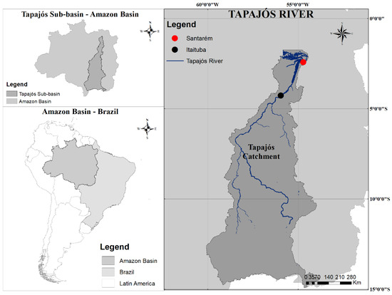
Figure 4.
Case study application area.
4.1. Models’ Water Level Forecast
The variable used for the data in question was the water level data from the Itaituba station, located in the Tapajós River. To obtain the forecast of water level data, daily data were collected from the Hidroweb platform of the Itaituba station from 1 February 1968 to 31 October 2019. Missing data were filled in for approximately 5.57% of the daily data.
The training process involved developing 20 perceptron neural networks with similar parameters, except for the number of neurons, which ranged from 1 neuron to a total of 35 neurons, distributed among up to five intermediate layers.
For the training of each model, a lag of 360 days was applied to make a forecast for the next 360 days. The inputs to the perceptron network were the current data on the given day plus the preceding 359 days. As output, the perceptron returned a vector containing the subsequent values, corresponding to approximately one year of forecast. The structure of the developed models, along with the generic metrics obtained for each model for the training process, is presented in Table 2, which illustrates the specific configurations of the neural network models used to predict water levels in this study. The model structure refers to the number of layers and the number of neurons in each layer of the multilayer perceptron (MLP) neural network, which is the artificial intelligence model employed.
Table 2.
Neural networking structure: MLP.
Each model listed in the table was trained using a different combination of neurons and intermediate layers. For instance, the MLP16, which showed the best performance with an R2 of 0.8761, has two intermediate layers containing six and four neurons, respectively. This structure refers to the number of neurons that process information and the organization of these layers within the neural network. Models with varying numbers of neurons and layers are tested to determine which configuration provides the most accurate predictions.
The structure directly influences the model’s ability to capture complex patterns in the data, such as seasonal variations in water levels. The goal was to find the optimal architecture that minimizes prediction errors and maximizes model accuracy, as reflected in the R2 and RMSE values presented in the table.
After creating the models, each model was trained using a subset of the data that was set aside for validation. Approximately 360 days of data were reserved exclusively for validation purposes, while the remaining dataset, consisting of 18,109 days, was used for training. During the training process, the models iteratively adjusted their weights and biases based on the training dataset, aiming to minimize the error between the predicted and actual water levels. The validation dataset was used to assess the performance and generalization capability of the trained models, providing an independent evaluation of their predictive accuracy. By using this approach, the MLP16 (Table 3) model with two intermediate layers and specific neuron configurations demonstrated superior performance compared to the other models in terms of accurately predicting water levels in the Itaituba station of the Tapajós River.
Table 3.
MLP16: Best ANN model characteristics.
4.2. Model Considerations
The model assumed that the seasonal fluctuation of water levels (flood and drought periods) was the primary determinant of available depths in the waterway. While this assumption holds true for much of the year, other factors can also significantly influence water depths. These included the following:
- Dynamic environmental and human factors: While the model focused on seasonal variations, real-world depths can be affected by sedimentation, dredging, and extreme weather events that may not align with seasonal patterns.
- Adaptive UKC and vessel configuration: The model assumed fixed parameters for UKC and convoy setup, which, in practice, may require adjustment depending on real-time river conditions and vessel behavior.
4.3. Project Vessel
For this study, specifically regarding the applicability to the lower Tapajós region, the larger and official dimensions of river convoys were adopted based on the guidelines of the Brazilian Navy, through the Command of the 4th Naval District. In their report on Rules and Procedures of River Captaincy—NPCF [82], the maximum dimensions of the vessel (pushboat and barges) are defined as a method to obtain the most unfavorable scenario for navigation on the Tapajós River, with a length of 343 m, width of 55 m, and draft of 3.70 m, as shown in Table 4.
Table 4.
River convoy characteristics.
5. Results and Discussions
5.1. Month Water Level Forecast
Using the methodological application for water level prediction using neural networks, R2 values were obtained for the evaluated models, with the best model achieving a generic R2 value of 0.8760713771767622. This model consisted of two intermediate layers with six and four neurons, respectively. Additionally, generic R2 and RMSE values were obtained for each training cycle, both on a daily and monthly basis, as shown in Figure 5.
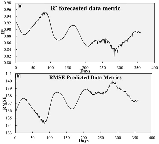
Figure 5.
R2 (a) and RMSE (b) metrics.
Regarding the obtained metrics, the output vector of the RNN models consists of 360 distinct values, meaning that the generic metric is calculated over all these values together. Each iterative process generates 360 connected values due to the structure of the neural networks, and there are a total of 360 data points for training. In computational terms, we have a vector of length 360, whose elements are other vectors of 360 distinct values. In mathematical terms, the values used to calculate the metric were derived from a 360 × 360 matrix, totaling 129,600 data points. A large amount of data tends to decrease the values obtained in the metrics.
For the purpose of discussion, the obtained individual metric graphs can be considered similar to a sinusoidal function, a first- or second-order linear function, and a randomly characterized error function. The sinusoidal shape of the R2 and RMSE metric values obtained confirms that the model was able to correlate the cyclical pattern present in the hydrological cycle. Even simpler models with only one neuron in the intermediate layer were also able to exhibit this behavior, which demonstrates that the cyclical nature of the historical series is easily “understood” by the model.
Regarding the noise generated in the individual metric graphs, different models showed similar noise patterns in different time periods. This may indicate that this noise also includes the results of the training process, a limitation of adaptation of the artificial neurons, in addition to the physical aspects of hydrology and the analyzed hydrological variable over time.
Figure 6 illustrates the comparisons between the actual values (x-axis) and the predicted values (y-axis) for the training cycles of the model that achieved the best results in the adopted evaluation metrics. Each training cycle is presented in each graph from left to right and top to bottom, with a graph interval every 50 cycles, aiming to highlight the trend of the predicted values approaching the actual values as the training cycles of the network progress.
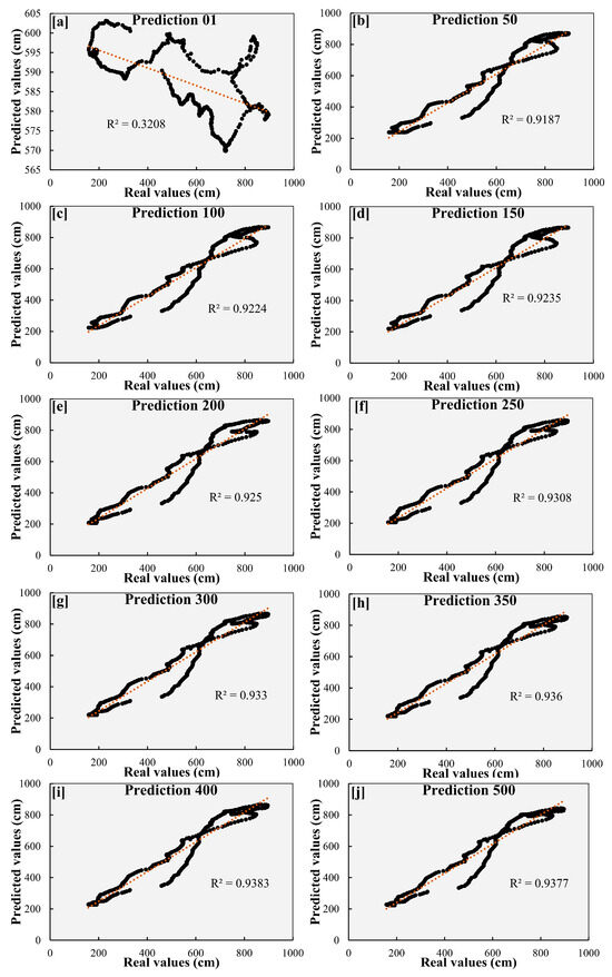
Figure 6.
Comparison between observed and predicted variables—from initial to final prediction (a–j).
Considering that the best prediction for the best model occurred approximately 83 days ahead, the obtained metrics for this specific prediction were an individual R2 of 0.954 and an individual RMSE of 0.095. Upon recovering the normalized data, we find that the mean error in the validation sample is 38.68 cm, with a maximum value of 101.25 cm and a minimum value of 0.032 cm. The values for the 25th, 50th, and 75th percentiles were 9.52 cm, 33.03 cm, and 60.49 cm, respectively. All subsequent statistical analyses are based on this 83-day prediction. The results can be better visualized in Figure 7.
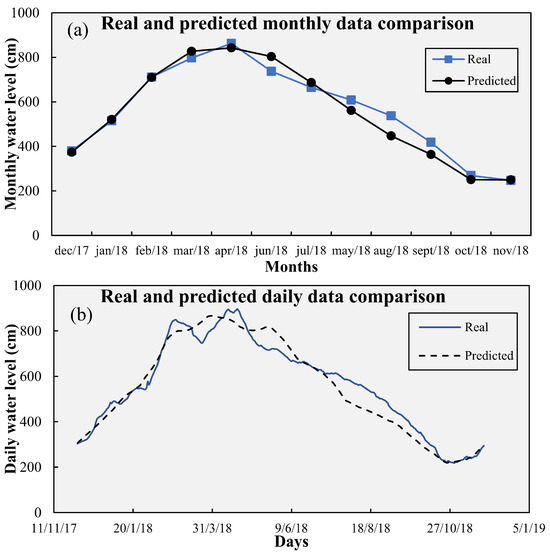
Figure 7.
Real and predicted data comparison.
5.2. Predicted Cargo Capacities
From the obtained daily water level values, it was possible to determine the predicted load capacities for the analyzed period (December 2017 to November 2018). To calculate these capacities, the influences of the squat effect were considered for each monthly depth situation, considering a constant under-keel clearance (UKC) of 0.9 m, calculated based on Eryuzlu et al. (1994). By subtracting the UKC values from the depth soundings, the available navigable draft for each month was determined, which allowed for obtaining the load capacities for the set of box barges, raked barges, and the convoy. The percentage of loading for each situation was calculated accordingly, as shown in Table 5.
Table 5.
Predicted movement capacities.
With the data obtained from Table 5, it was possible to verify the months with critical navigation, where lower depths were observed between August and December, corresponding to the dry season when the river is influenced by the seasonality of the Amazonian watercourses. In August, the water begins to recede, marking the beginning of the dry season, which becomes more pronounced in October when temperatures also start to rise.
By modeling these cargo capacities, it is possible to identify the periods when navigation with maximum capacities is not possible. This is extremely relevant for navigation in this region, as it involves continuous navigation, particularly for the transportation of agricultural crops (such as soybeans and corn) from the Midwest region of Brazil.
5.3. Navigation Restrictions
Another extremely relevant point enabled by determining the river water levels and, consequently, their cargo-carrying capacities is the assessment of critical navigation sections observed during scenarios of lower depths. These critical sections occur not only due to depth limitations but also due to width limitations resulting from reduced water levels. Thus, to spatialize these critical sections, it was possible to determine two analysis scenarios for the dry months. The first scenario, called moderate, consisted of the months of August, September, and December, and the second scenario, called critical, consisted of the months of October and November. The modeling of the rivers was performed based on the development of a digital elevation model, which allowed the identification of critical sections in Figure 8, with the red regions representing areas where navigation is impeded in that scenario and the blue regions representing areas with navigation possibilities.
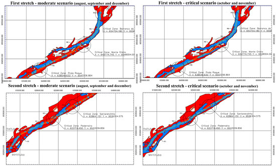
Figure 8.
Critical sections spatialization (Blue = stretch without restriction; Red = stretch with restriction).
Regarding the analyzed scenarios, it can be observed that in October and November, due to lower water levels, the red regions are more exposed, representing greater navigation restrictions. While in August, September, and December, the red regions are reduced but still have navigation restrictions. It should be noted that the other months were not represented because they do not have navigation restrictions, allowing navigation with the maximum capacity of the convoys.
From the identification of the observed sections in Figure 8, it can be noticed that there are five critical sections, named Perderneira, Santarénzinho, Praia Roque, Monte Cristo, and Barranco do Navio, which are evidenced in both scenarios as regions with width and depth restrictions for the adopted analysis environment. The regions with highlighted restrictions in the spatialization of the navigation channel layout are characterized as critical zones with depth restrictions already identified by the Brazilian Navy, which corroborated the obtained results.
6. Conclusions
The present article presents a computational model based on a multilayer perceptron artificial neural network (ANN) with the main objective of obtaining the cargo-carrying capacities of a river convoy for a given waterway based on water level predictions to verify the seasonality of the river course. Coupled with the modeling of the hydrostatic characteristics of the vessel design and the planialtimetric characteristics of the river, this model enables the verification of navigation bottlenecks, as well as the knowledge of periods when the river course will have navigation restrictions, which represent capacity losses and, eventually, an increase in the cost of transportation and the transported product. Additionally, the model supports environmental sustainability by optimizing river logistics to minimize fuel consumption and emissions, thus reducing the ecological footprint of river transportation.
The results obtained from the multilayer perceptron artificial neural network (MLP-ANN) model demonstrate a high level of reliability, with an R2 of 0.954 and RMSE of 0.095. These metrics indicate that the model is effective in predicting water levels and cargo capacities in the Tapajós River, accurately capturing the seasonal hydrological variations in the region.
When compared to similar studies, such as the application of random forest models by Garcia et al. [52] on the Cagayan River and the ARIMA models used by Figueiredo and Blanco [50] for the Tapajós River, the MLP-ANN model shows similar predictive performance. While these previous models provided valuable insights, they often struggled to account for the extreme seasonal variability characteristic of the Amazon Basin. The enhanced accuracy of the MLP-ANN model underscores its ability to provide more consistent and reliable predictions for river logistics management.
Despite the promising outcomes, this study has some limitations. The accuracy of the model is highly dependent on the quality of historical water level data. Any gaps or inaccuracies in this data could affect the model’s performance. Additionally, while the model was specifically calibrated for the Tapajós River, applying it to other rivers with different hydrological characteristics would require additional validation. The model currently focuses on technical predictions and does not fully integrate economic or environmental variables, such as fuel costs or emissions, which could offer a more comprehensive understanding of river logistics.
Future research should focus on overcoming these limitations and expanding the model’s applicability. Integrating real-time hydrological data could enhance the model’s accuracy and responsiveness to sudden changes in water levels, making it more useful for managing unexpected events like floods or droughts. Expanding the application of the model to other rivers, both within and outside the Amazon Basin, is also essential. This would involve adapting the model to different hydrological conditions and validating its performance in these new contexts. Finally, incorporating economic and environmental factors into the model would provide more holistic support for decision-making, balancing operational efficiency with sustainability goals.
This study successfully developed a robust and accurate machine learning model for predicting water levels and cargo capacities in the Tapajós River. The MLP-ANN model outperforms existing approaches and offers valuable insights for optimizing river logistics. Further research is needed to expand the model’s applicability, enhance its predictive capabilities, and integrate additional variables that reflect the economic and environmental dimensions of river transportation.
Therefore, concerning the objectives of this article, they were achieved; the validation of the model proved satisfactory given the obtained results, and the computational routine based on ANN proved to be a tool capable of enhancing navigation safety as well as enabling the prediction of periods with less or more significant navigation restrictions. This research contributes to the assessment and mitigation of impacts related to dry periods in rivers, which are crucial for the economic development of the analyzed area, thus supporting sustainable management and development initiatives.
Author Contributions
L.C.P.C.F.: conceptualization, methodology, software, and formal analysis; N.M.d.F.: methodology, supervision, and formal analysis; C.J.C.B.: supervision and writing—reviewing; M.S.G.T.: technical discussions, supervision, and writing—reviewing.; and P.A.: conceptualization, technical discussions, supervision, and writing—reviewing. All authors have read and agreed to the published version of the manuscript.
Funding
This work was supported by the Coordination for the Improvement of Higher Education Personnel Foundation (CAPES) and Postgraduate Program in Civil Engineering (PPGEC) of the Federal University of Pará (UFPA).
Institutional Review Board Statement
Not applicable.
Informed Consent Statement
Not applicable.
Data Availability Statement
Data are contained within the article.
Acknowledgments
The authors acknowledge the contribution to this work made by members of the research team named “Waterway and Port Research Group” from the Institute of Technology-Federal University of Pará and the ALGORITMI Center, Department of Production and Systems, University of Minho, for support in carrying out the research, in the availability of software for data generation, and in contributions to the technical discussion of the results.
Conflicts of Interest
The authors declare no conflicts of interest.
References
- Taylor, N.B. Book Review. J. Transp. Geogr. 2018, 69, 307. [Google Scholar] [CrossRef]
- Williamsson, J.; Rogerson, S.; Santén, V. Business Models for Dedicated Container Freight on Swedish Inland Waterways. Res. Transp. Bus. Manag. 2020, 35, 100466. [Google Scholar] [CrossRef]
- Medda, F.; Trujillo, L. Short-Sea Shipping: An Analysis of Its Determinants. Marit. Policy Manag. 2010, 37, 285–303. [Google Scholar] [CrossRef]
- Suárez-Alemán, A.; Trujillo, L.; Medda, F. Short Sea Shipping as Intermodal Competitor: A Theoretical Analysis of European Transport Policies. Marit. Policy Manag. 2015, 42, 317–334. [Google Scholar] [CrossRef]
- Wiegmans, B.; Konings, R. Intermodal Inland Waterway Transport: Modelling Conditions Influencing Its Cost Competitiveness. Asian J. Shipp. Logist. 2015, 31, 273–294. [Google Scholar] [CrossRef]
- Solomon, B.; Otoo, E.; Boateng, A.; Ato Koomson, D. Inland Waterway Transportation (IWT) in Ghana: A Case Study of Volta Lake Transport. Int. J. Transp. Sci. Technol. 2020, 10, 20–33. [Google Scholar] [CrossRef]
- Tvedt, T. Why England and Not China and India? Water Systems and the History of the Industrial Revolution. J. Glob. Hist. 2010, 5, 29–50. [Google Scholar] [CrossRef][Green Version]
- Sakalis, G.N.; Frangopoulos, C.A. Intertemporal Optimization of Synthesis, Design and Operation of Integrated Energy Systems of Ships: General Method and Application on a System with Diesel Main Engines. Appl. Energy 2018, 226, 991–1008. [Google Scholar] [CrossRef]
- Ahadi, K.; Sullivan, K.M.; Mitchell, K.N. Budgeting Maintenance Dredging Projects under Uncertainty to Improve the Inland Waterway Network Performance. Transp. Res. Part E Logist. Transp. Rev. 2018, 119, 63–87. [Google Scholar] [CrossRef]
- Segovia, P.; Rajaoarisoa, L.; Nejjari, F.; Duviella, E.; Puig, V. Model Predictive Control and Moving Horizon Estimation for Water Level Regulation in Inland Waterways. J. Process Control 2019, 76, 1–14. [Google Scholar] [CrossRef]
- Teixeira, C.A.N.; Rocio, M.A.R.; do Amaral, A.P.; d’Oliveira, L.A.S. Brazilian Inland Navigation. Available online: https://web.bndes.gov.br/bib/jspui/bitstream/1408/15380/3/BS47__NavegacaoInterior_P.pdf (accessed on 4 May 2024).
- Duldner-Borca, B.; Hoerandner, L.; Bieringer, B.; Khanbilverdi, R.; Putz-Egger, L.-M. New Design Options for Container Barges with Improved Navigability on the Danube. Sustainability 2024, 16, 4613. [Google Scholar] [CrossRef]
- Shi, J.; Bai, T.; Zhao, Z.; Tan, H. Driving Economic Growth through Transportation Infrastructure: An In-Depth Spatial Econometric Analysis. Sustainability 2024, 16, 4283. [Google Scholar] [CrossRef]
- Hunt, J.D.; Pokhrel, Y.; Chaudhari, S.; Mesquita, A.L.A.; Nascimento, A.; Leal Filho, W.; Biato, M.F.; Schneider, P.S.; Lopes, M.A. Challenges and Opportunities for a South America Waterway System. Clean. Eng. Technol. 2022, 11, 100575. [Google Scholar] [CrossRef]
- Vilarinho, A.; Liboni, L.B.; Cezarino, L.O.; Micco, J.D.; Mommens, K.; Macharis, C. Challenges and Opportunities for the Development of Inland Waterway Transport in Brazil. Sustainability 2024, 16, 2136. [Google Scholar] [CrossRef]
- Chen, Y.; Zhou, B.; Pan, X.; Zhang, H.; Qian, H.; Cheng, W.; Yin, W. Assessing Waterway Carrying Capacity from a Multi-Benefit Synergistic Perspective. Sustainability 2024, 16, 4379. [Google Scholar] [CrossRef]
- Lalla-Ruiz, E.; Shi, X.; Voß, S. The Waterway Ship Scheduling Problem. Transp. Res. Part D Transp. Environ. 2018, 60, 191–209. [Google Scholar] [CrossRef]
- Lindstad, H.E.; Sandaas, I. Emission and Fuel Reduction for Offshore Support Vessels through Hybrid Technology. J. Ship Prod. Des. 2016, 32, 195–205. [Google Scholar] [CrossRef]
- Ling-Chin, J.; Roskilly, A.P. Investigating the Implications of a New-Build Hybrid Power System for Roll-on/Roll-off Cargo Ships from a Sustainability Perspective—A Life Cycle Assessment Case Study. Appl. Energy 2016, 181, 416–434. [Google Scholar] [CrossRef]
- Dedes, E.K.; Hudson, D.A.; Turnock, S.R. Investigation of Diesel Hybrid Systems for Fuel Oil Reduction in Slow Speed Ocean Going Ships. Energy 2016, 114, 444–456. [Google Scholar] [CrossRef]
- Talluri, L.; Nalianda, D.K.; Kyprianidis, K.G.; Nikolaidis, T.; Pilidis, P. Techno Economic and Environmental Assessment of Wind Assisted Marine Propulsion Systems. Ocean Eng. 2016, 121, 301–311. [Google Scholar] [CrossRef]
- Almaz, O.A.; Altiok, T. Simulation Modeling of the Vessel Traffic in Delaware River: Impact of Deepening on Port Performance. Simul. Model. Pract. Theory 2012, 22, 146–165. [Google Scholar] [CrossRef]
- Fathoni, M.; Pradono, P.; Syabri, I.; Shanty, Y.R. Analysis to Assess Potential Rivers for Cargo Transport in Indonesia. Transp. Res. Procedia 2017, 25, 4544–4559. [Google Scholar] [CrossRef]
- Kamal, N.; Sadek, N. Evaluating and Analyzing Navigation Efficiency for the River Nile (Case Study: Ensa-Naga Hamady Reach). Ain Shams Eng. J. 2018, 9, 2649–2669. [Google Scholar] [CrossRef]
- Kuo, C.C.; Gan, T.Y.; Higuchi, K. Evaluation of Future Streamflow Patterns in Lake Simcoe Subbasins Based on Ensembles of Statistical Downscaling. J. Hydrol. Eng. 2017, 22, 04017028. [Google Scholar] [CrossRef]
- Scheepers, H.; Wang, J.; Gan, T.Y.; Kuo, C.C. The Impact of Climate Change on Inland Waterway Transport: Effects of Low Water Levels on the Mackenzie River. J. Hydrol. 2018, 566, 285–298. [Google Scholar] [CrossRef]
- Sugeng, S. Dampak pelayaran kapal laut di alur Sungai Musi. Gema Teknol. 2010, 16, 49–56. [Google Scholar] [CrossRef]
- Zuo, L.; Lu, Y.; Liu, H.; Ren, F.; Sun, Y. Responses of River Bed Evolution to Flow-Sediment Process Changes after Three Gorges Project in Middle Yangtze River: A Case Study of Yaojian Reach. Water Sci. Eng. 2020, 13, 124–135. [Google Scholar] [CrossRef]
- Luo, X.; Zhang, W.; Chen, S.; Feng, X.; Ji, X.; Xu, Y. Evolution of Reversal of the Lowest Low Waters in a Tidal River Network. J. Hydrol. 2020, 585, 124701. [Google Scholar] [CrossRef]
- Nasir, H.A.; Zhao, T.; Carè, A.; Wang, Q.J.; Weyer, E. Efficient River Management Using Stochastic MPC and Ensemble Forecast of Uncertain In-Flows. IFAC-PapersOnLine 2018, 51, 37–42. [Google Scholar] [CrossRef]
- Christodoulou, A.; Christidis, P.; Bisselink, B. Forecasting the Impacts of Climate Change on Inland Waterways. Transp. Res. Part D Transp. Environ. 2020, 82, 102159. [Google Scholar] [CrossRef]
- Nouasse, H.; Doniec, A.; Lozenguez, G.; Duviella, E.; Chiron, P.; Archimède, B.; Chuquet, K. Constraint Satisfaction Problem Based on Flow Graph to Study the Resilience of Inland Navigation Networks in a Climate Change context. IFAC-PapersOnLine 2016, 49, 331–336. [Google Scholar] [CrossRef]
- Vidyalashmi, K.; Chandana L, M.; Nandana, J.S.; Azhikodan, G.; Priya, K.L.; Yokoyama, K.; Paramasivam, S.K. Analysing the Performance of the NARX Model for Forecasting the Water Level in the Chikugo River Estuary, Japan. Environ. Res. 2024, 251, 118531. [Google Scholar] [CrossRef] [PubMed]
- Liu, W.-C.; Huang, W.-C. Evaluation of Deep Learning Computer Vision for Water Level Measurements in Rivers. Heliyon 2024, 10, e25989. [Google Scholar] [CrossRef]
- Li, G.; Zhu, H.; Jian, H.; Zha, W.; Wang, J.; Shu, Z.; Yao, S.; Han, H. A Combined Hydrodynamic Model and Deep Learning Method to Predict Water Level in Ungauged Rivers. J. Hydrol. 2023, 625, 130025. [Google Scholar] [CrossRef]
- Wang, X.; Xia, J.; Zhou, M.; Deng, S.; Li, Q. Assessment of the Joint Impact of Rainfall and River Water Level on Urban Flooding in Wuhan City, China. J. Hydrol. 2022, 613, 128419. [Google Scholar] [CrossRef]
- Moges, D.M.; Kmoch, A.; Uuemaa, E. Application of Satellite and Reanalysis Precipitation Products for Hydrological Modeling in the Data-Scarce Porijõgi Catchment, Estonia. J. Hydrol. Reg. Stud. 2022, 41, 101070. [Google Scholar] [CrossRef]
- Sikora de Souza, V.A.; Moreira, D.M.; Rotunno Filho, O.C.; Rudke, A.P. Extreme Rainfall Events in Amazonia: The Madeira River Basin. Remote Sens. Appl. Soc. Environ. 2020, 18, 100316. [Google Scholar] [CrossRef]
- Ahmed, K.; Shahid, S.; Nawaz, N.; Khan, N. Modeling Climate Change Impacts on Precipitation in Arid Regions of Pakistan: A Non-Local Model Output Statistics Downscaling Approach. Theor. Appl. Climatol. 2019, 137, 1347–1364. [Google Scholar] [CrossRef]
- Ahmed, K.; Shahid, S.; Wang, X.; Nawaz, N.; Khan, N. Evaluation of Gridded Precipitation Datasets over Arid Regions of Pakistan. Water 2019, 11, 210. [Google Scholar] [CrossRef]
- Latif, M.; Syed, F.; Hannachi, A. Rainfall Trends in the South Asian Summer Monsoon and Its Related Large-Scale Dynamics with Focus over Pakistan. Clim. Dyn. 2017, 48, 3565–3581. [Google Scholar] [CrossRef]
- Dinku, T.; Funk, C.; Peterson, P.; Maidment, R.; Tadesse, T.; Gadain, H.; Ceccato, P. Validation of the CHIRPS Satellite Rainfall Estimates over Eastern Africa. Q. J. R. Meteorol. Soc. 2018, 144, 292–312. [Google Scholar] [CrossRef]
- Funk, C.; Peterson, P.; Landsfeld, M.; Pedreros, D.; Verdin, J.; Shukla, S.; Husak, G.; Rowland, J.; Harrison, L.; Hoell, A.; et al. The Climate Hazards Infrared Precipitation with Stations—A New Environmental Record for Monitoring Extremes. Sci. Data 2015, 2, 150066. [Google Scholar] [CrossRef] [PubMed]
- Zambrano, F.; Wardlow, B.; Tadesse, T.; Lillo-Saavedra, M.; Lagos, O. Evaluating Satellite-Derived Long-Term Historical Precipitation Datasets for Drought Monitoring in Chile. Atmos. Res. 2017, 186, 26–42. [Google Scholar] [CrossRef]
- Seo, Y.J.; Ha, M.H.; Yang, Z.; Bhattacharya, S. The Ship Management Firm Selection: The Case of South Korea. Asian J. Shipp. Logist. 2018, 34, 256–265. [Google Scholar] [CrossRef]
- Le Carrer, N.; Ferson, S.; Green, P.L. Optimising Cargo Loading and Ship Scheduling in Tidal Areas. Eur. J. Oper. Res. 2020, 280, 1082–1094. [Google Scholar] [CrossRef]
- Li, B.; Yang, G.; Wan, R.; Dai, X.; Zhang, Y. Comparison of Random Forests and Other Statistical Methods for the Prediction of Lake Water Level: A Case Study of the Poyang Lake in China. Hydrol. Res. 2016, 47, 69–83. [Google Scholar] [CrossRef]
- Khan, M.Y.A.; Hasan, F.; Panwar, S.; Chakrapani, G.J. Neural Network Model for Discharge and Water-Level Prediction for Ramganga River Catchment of Ganga Basin, India. Hydrol. Sci. J. 2016, 61, 2084–2095. [Google Scholar] [CrossRef]
- Phan, T.-T.-H.; Nguyen, X.H. Combining Statistical Machine Learning Models with ARIMA for Water Level Forecasting: The Case of the Red River. Adv. Water Resour. 2020, 142, 103656. [Google Scholar] [CrossRef]
- Figueiredo, N.; Blanco, C. Simulação de Vazões e Níveis de Água Médios Mensais Para o Rio Tapajós Usando Modelos ARIMA. Rev. Bras. Recur. Hidr. 2014, 19, 111–126. [Google Scholar] [CrossRef]
- Barbosa, F.G.P.; de Figueiredo, N.M.; Filho, L.C.P.C.; Borges, H.M. Computational Tool for Sizing and Optimization of Planimetric Geometric Parameters of Inland Navigation Channels and of Port Access in Brazil. J. Waterw. Port Coast. Ocean Eng. 2021, 147, 04020044. [Google Scholar] [CrossRef]
- Garcia, F.C.C.; Retamar, A.E.; Javier, J.C. Development of a Predictive Model for On-Demand Remote River Level Nowcasting: Case Study in Cagayan River Basin, Philippines. In Proceedings of the 2016 IEEE Region 10 Conference (TENCON), Singapore, 22–25 November 2016; pp. 3275–3279. [Google Scholar]
- Wang, L.; Wu, B.; Zhu, Q.; Zeng, Y.-R. Forecasting Monthly Tourism Demand Using Enhanced Backpropagation Neural Network. Neural Process. Lett. 2020, 52, 2607–2636. [Google Scholar] [CrossRef]
- Li, T.; Wang, S.; Liu, Y.; Fu, B.; Gao, D. Reversal of the Sediment Load Increase in the Amazon Basin Influenced by Divergent Trends of Sediment Transport from the Solimões and Madeira Rivers. Catena 2020, 195, 104804. [Google Scholar] [CrossRef]
- Feng, X.; Ma, G.; Su, S.-F.; Huang, C.; Boswell, M.K.; Xue, P. A Multi-Layer Perceptron Approach for Accelerated Wave Forecasting in Lake Michigan. Ocean Eng. 2020, 211, 107526. [Google Scholar] [CrossRef]
- Hunasigi, P.; Jedhe, S.; Mane, M.; Patil-Shinde, V. Multilayer Perceptron Neural Network Based Models for Prediction of the Rainfall and Reference Crop Evapotranspiration for Sub-Humid Climate of Dapoli, Ratnagiri District, India. Acta Ecol. Sin. 2022, 43, 154–201. [Google Scholar] [CrossRef]
- Haykin, S.S. Neural Networks: A Comprehensive Foundation, 2nd ed.; Prentice Hall: Upper Saddle River, NJ, USA, 1999; ISBN 978-0-13-273350-2. [Google Scholar]
- Chen, C.-S.; Chen, B.P.-T.; Chou, F.N.-F.; Yang, C.-C. Development and Application of a Decision Group Back-Propagation Neural Network for Flood Forecasting. J. Hydrol. 2010, 385, 173–182. [Google Scholar] [CrossRef]
- Petrosyan, A.; Dereventsov, A.; Webster, C.G. Neural Network Integral Representations with the ReLU Activation Function. In Proceedings of the First Mathematical and Scientific Machine Learning Conference, Virtual, 16–19 August 2020; pp. 128–143. [Google Scholar]
- Schmidt-Hieber, J. Nonparametric Regression Using Deep Neural Networks with ReLU Activation Function. Ann. Stat. 2020, 48, 1875–1897. [Google Scholar] [CrossRef]
- Boob, D.; Dey, S.S.; Lan, G. Complexity of Training ReLU Neural Network. Discret. Optim. 2020, 44, 100620. [Google Scholar] [CrossRef]
- Lin, G.; Shen, W. Research on Convolutional Neural Network Based on Improved Relu Piecewise Activation Function. Procedia Comput. Sci. 2018, 131, 977–984. [Google Scholar] [CrossRef]
- Kingma, D.P.; Ba, J. Adam: A Method for Stochastic Optimization. arXiv 2017, arXiv:1412.6980. [Google Scholar]
- Azad, A.; Pirayesh, J.; Farzin, S.; Malekani, L.; Moradinasab, S.; Kisi, O. Application of Heuristic Algorithms in Improving Performance of Soft Computing Models for Prediction of Min, Mean and Max Air Temperatures. Eng. J. 2019, 23, 83–98. [Google Scholar] [CrossRef]
- Wang, J.; Shi, P.; Jiang, P.; Hu, J.; Qu, S.; Chen, X.; Chen, Y.; Dai, Y.; Xiao, Z. Application of BP Neural Network Algorithm in Traditional Hydrological Model for Flood Forecasting. Water 2017, 9, 48. [Google Scholar] [CrossRef]
- Abrahart, R.J.; White, S.M. Modelling Sediment Transfer in Malawi: Comparing Backpropagation Neural Network Solutions against a Multiple Linear Regression Benchmark Using Small Data Sets. Phys. Chem. Earth Part B Hydrol. Ocean. Atmos. 2001, 26, 19–24. [Google Scholar] [CrossRef]
- Wang, Z.; Sheng, H. Rainfall Prediction Using Generalized Regression Neural Network: Case Study Zhengzhou. In Proceedings of the 2010 International Conference on Computational and Information Sciences, Chengdu, China, 17–19 December 2010; pp. 1265–1268. [Google Scholar]
- Nourani, V. An Emotional ANN (EANN) Approach to Modeling Rainfall-Runoff Process. J. Hydrol. 2017, 544, 267–277. [Google Scholar] [CrossRef]
- Sahoo, B.B.; Jha, R.; Singh, A.; Kumar, D. Long Short-Term Memory (LSTM) Recurrent Neural Network for Low-Flow Hydrological Time Series Forecasting. Acta Geophys. 2019, 67, 1471–1481. [Google Scholar] [CrossRef]
- Valipour, M.; Banihabib, M.E.; Behbahani, S.M.R. Comparison of the ARMA, ARIMA, and the Autoregressive Artificial Neural Network Models in Forecasting the Monthly Inflow of Dez Dam Reservoir. J. Hydrol. 2013, 476, 433–441. [Google Scholar] [CrossRef]
- Kumar, U.A. Comparison of Neural Networks and Regression Analysis: A New Insight. Expert Syst. Appl. 2005, 29, 424–430. [Google Scholar] [CrossRef]
- Coulibaly, P.; Bobée, B.; Anctil, F. Improving Extreme Hydrologic Events Forecasting Using a New Criterion for Artificial Neural Network Selection. Hydrol. Process. 2001, 15, 1533–1536. [Google Scholar] [CrossRef]
- Barrass, C.B.; Derrett, D.R. Hydrostatic Curves and Values for Vessels Initially Having Trim by the Bow or by the Stern. In Ship Stability for Masters and Mates; Elsevier: Amsterdam, The Netherlands, 2012; pp. 235–240. ISBN 978-0-08-097093-6. [Google Scholar]
- Biran, A.; López-Pulido, R. Hydrostatic Curves. In Ship Hydrostatics and Stability; Elsevier: Amsterdam, The Netherlands, 2014; pp. 97–116. ISBN 978-0-08-098287-8. [Google Scholar]
- Tupper, E.C. Structures. In Introduction to Naval Architecture; Elsevier: Amsterdam, The Netherlands, 2013; pp. 299–341. ISBN 978-0-08-098237-3. [Google Scholar]
- Adland, R.; Jia, H.; Strandenes, S.P. The Determinants of Vessel Capacity Utilization: The Case of Brazilian Iron Ore Exports. Transp. Res. Part A Policy Pract. 2018, 110, 191–201. [Google Scholar] [CrossRef]
- Campos Filho, L.C.P.; Moura de Figueiredo, N.; Pantoja Barbosa, F.G.; Saavedra, R.d.S.; Filgueiras, T.; Pavão de Souza, P.A. Analysis of Geometric Conformation of the Lower Tapajós Stretch Using Navigation Channel Sizing Software; Galoa: Brasília, Brazil, 2019. [Google Scholar]
- PIANC. Harbour Approach Channels Design Guidelines, PIANC Report No. 121; PIANC: Brussels, Belgium, 2014; ISBN 978-2-87223-210-9. [Google Scholar]
- Briggs, M.J.; Vantorre, M.; Uliczka, K.; Debaillon, P. Prediction of Squat for Underkeel Clearance. In Handbook of Coastal and Ocean Engineering; World Scientific: Singapore, 2018; pp. 1029–1080. ISBN 978-981-320-401-0. [Google Scholar]
- Briggs, M.J.; Silver, A.; Kopp, P.J.; Santangelo, F.A.; Mathis, I.A. Validation of a Risk-Based Numerical Model for Predicting Deep-Draft Underkeel Clearance. J. Waterw. Port Coast. Ocean Eng. 2013, 139, 267–276. [Google Scholar] [CrossRef]
- Eryuzlu, N.E.; Cao, Y.L.; D’Agnolo, F. Underkeel Requirements for Large Vessels in Shallow Waterways. In Proceedings of the 28th International Navigation Congress, Sevilla, Spain, 10 May 1994; pp. 17–25. [Google Scholar]
- Capitania Fluvial de Porto Velho. Normas e Procedimentos específicos para a jurisdição da Capitania Fluvial de Porto Velho. Available online: https://www.marinha.mil.br/cfpv/?q=conteudo/normas-e-procedimentos-especificos-para-jurisdicao-da-capitania-fluvial-de-porto-velho (accessed on 4 May 2024).


Disclaimer/Publisher’s Note: The statements, opinions and data contained in all publications are solely those of the individual author(s) and contributor(s) and not of MDPI and/or the editor(s). MDPI and/or the editor(s) disclaim responsibility for any injury to people or property resulting from any ideas, methods, instructions or products referred to in the content. |
© 2024 by the authors. Licensee MDPI, Basel, Switzerland. This article is an open access article distributed under the terms and conditions of the Creative Commons Attribution (CC BY) license (https://creativecommons.org/licenses/by/4.0/).