Abstract
CO2 emission is a big problem, not only for current living beings, but also for nature and the upcoming generations. Therefore, modeling CO2 emissions is the first step in reducing these emissions. In this work, the CO2 emissions of Turkey are modeled depending on the gross domestic product, amount of hydroelectric electricity generated, amount of energy generated from coal and the electricity obtained from natural gas power plants. The conventional autoregressive integrated moving average with exogenous variables (ARIMAX) and nonlinear deep learning methods are utilized to model CO2 emissions for the period of 1960–2020 using yearly data obtained from official sources. The modeling results of the ARIMAX and the deep learning methods are quantitatively assessed using four key figures of merit, namely the coefficient of determination (R2), mean absolute error (MAE), mean absolute percentage error (MAPE) and the root mean square error (RMSE). Considering the coefficient of determination and the other performance parameters, it is observed that the deep learning model provides better performance compared with the ARIMAX model in modeling the annual CO2 emission data, especially in the pandemic period of 2019–2020. The results show that both the conventional ARIMAX and the nonlinear deep learning methods can be utilized to model CO2 emissions, therefore providing a crucial step for reducing CO2 emissions and the carbon footprint.
1. Introduction
Environmental quality is an important indicator of the development and civilization status of countries. The forerunner of environmental pollution is greenhouse gas emissions, where CO2 emissions have the largest share. Greenhouse gases are emitted into the atmosphere as a result of economic production processes, and then these gases cause the greenhouse effect, which leads to climate changes and the increment in average temperatures. The relationship between economic income and environmental pollution is generally modeled using the hypothesis called the environmental Kuznets curve (EKC). This hypothesis expresses that the level of environmental degradation in underdeveloped and developed countries is low, while the pollution caused by developing countries is higher. In fact, this hypothesis is derived from the original Kuznets curve hypothesis, which explains that economic inequality has an inverse U-shaped curve dependent on income per capita [1]. The environmental Kuznets curve hypothesis was proposed by Grossman and Krueger in 1991 [2]. From this viewpoint, it is vital to assess the environmental Kuznets curve analysis of Turkey, as it is a rapidly developing country with a high level of economic growth [3,4]. The original environmental Kuznets curve hypothesis includes economic growth as the independent variable and the level of environmental degradation as the dependent variable, while an inverted U-shaped curve is expected between these variables [2].
Our study delves into the critical issue of environmental degradation, specifically focusing on CO2 emissions as a primary indicator of this phenomenon from a sustainability viewpoint. The background of this study is grounded in the growing global concern over climate change and the detrimental effects of greenhouse gas emissions, which are predominantly driven by economic activities. Over the years, numerous studies have highlighted the strong correlation between economic growth, energy production and environmental degradation, particularly CO2 emissions. However, the complexity of these relationships, especially the nonlinear interactions between economic variables and environmental outcomes, necessitates more sophisticated modeling approaches, as given in detail in the following literature survey section. The rationale for this study stems from the need to improve predictive models that can more accurately capture these relationships, thereby providing valuable insights for policymakers. By comparing the performance of conventional statistical models like ARIMAX with advanced deep learning methods, the authors aim to determine the most effective approach for modeling CO2 emissions. This is crucial for devising strategies to mitigate the impact of economic activities on the environment and to contribute to the global effort to reduce greenhouse gas emissions.
The aim of this study is to model the level of environmental degradation using economic variables. CO2 emissions are taken as the indicator for the level of environmental degradation, while the independent variables are selected as the gross domestic product per capita and the electricity generated using coal, hydroelectric power plants and natural gas. The conventional autoregressive integrated moving average with exogenous variables (ARIMAX) and nonlinear deep learning methods are utilized to model CO2 emissions dependent on the gross domestic product per capita and the electricity generated using coal, hydroelectric power plants and natural gas. Furthermore, the figures of merits of these models such as the coefficient of determination (R2), mean absolute error (MAE), mean absolute percentage error (MAPE) and the root mean square error (RMSE) are computed. The modeling results show that CO2 emissions can be accurately modeled by both the ARIMAX and deep learning methods, which is significant in understanding the factors affecting CO2 emissions to reduce greenhouse gases.
2. Literature Survey
The uncontrolled greenhouse gas emissions from industrial production and oil-based vehicles increase the level of environmental degradation. This process was accelerated by the rapid industrialization of countries after World War II, which led to discussions of the scientific evidence for climate changes at the United Nations General Assembly in 1968 and then the Stockholm Conference in 1972, which aimed to address environmental problems with international collaboration [5]. Then, the climate change effects and the potential prevention measures were discussed in detail in 1987, and the report named Our Common Future was published by the Brutland Commission [6]. Furthermore, the Kyoto Protocol was signed by 84 countries in 1997; however, the results of this protocol were limited because only 46 countries ratified the protocol, including the European Union countries and Japan, while industrialized countries such as China, the United States and Australia did not ratify the protocol [7]. Finally, the Paris Agreement, which is a legally binding international treaty to combat climate change, was signed by 196 countries at the UN Climate Change Conference in 2015. The Paris Agreement came into force on 4 November 2016 and aims to hold “the increase in the global average temperature to well below 2 °C above pre-industrial levels” and pursue efforts “to limit the temperature increase to 1.5 °C above pre-industrial levels”. [8]. Turkey has also ratified the Paris Agreement and aims to reduce its total greenhouse gas emissions from the projected 1175 Mt (million tons) to 929 Mt by 2030 [9]. This corresponds to a 21% reduction in total greenhouse gas emissions. It is obviously important to model the greenhouse gas emissions to achieve accurate predictions for the future. Therefore, it is imperative to analyze the main causes and their share in the greenhouse emissions. The studies existing in the literature indicate that the biggest contributor to CO2 emissions of Turkey is the economic expansion, in other words the scale effect, caused by the increase in the energy production [10]. This is in line with other territories such as the European Union for which it is reported that the industrial processes and the energy production are named as the source of the greenhouse gas emissions [11]. Hence, it is possible to model the greenhouse gas emissions, particularly CO2 emissions since it has the largest share dependent on the economic growth and the consumption of the fuels for energy production. This modeling not only helps to understand the contributions of various factors to CO2 gas emissions but also enables us to forecast CO2 emissions, which aids the policies for the reduction in greenhouse gas emissions according to the Paris Agreement.
There are vast numbers of studies in the literature regarding the assessment of the environmental Kuznets curve hypothesis. In one of these studies, the income per capita and the greenhouse gas emissions for the United States are considered in the period of 1988–1994, where it is shown that the level of environmental degradation decreases as the income per capita increases, which is in line with the environmental Kuznets curve hypothesis [12]. CO2 emissions and the economic growth of China for the 1991–2006 period are investigated in another study in which it is concluded that the economic scaling has important effects on the level of environmental degradation in China, which is the second country for the greenhouse gas emissions viewpoint [13]. The economies and the air pollution data of 18 selected OECD countries are analyzed in another work employing the panel data analysis method where it is shown that the economic growth and the greenhouse gas emissions data of these countries support the environmental Kuznets curve hypothesis [14]. The empirical study of Bruvoll and Medin also verifies that there is a correlation between the income per capita and the environmental pollution for the developed countries, also verifying the environmental Kuznets curve hypothesis [15]. In another study, it is argued that the environmental degradation increases monotonically in low-income countries and decreases monotonically in high-income countries, while having inverted U characteristics for middle-income countries, as estimated by the environmental Kuznets curve (EKC) hypothesis [16]. The environmental Kuznets curve hypothesis was also studied by Burnett et al. where they have considered the monthly CO2 emission and income per capita data of the United States for the period of 1981–2003 and they have validated the EKC hypothesis [17]. The causality relationship between CO2 emission and the economic growth is also studied in the literature in conjunction with the environmental Kuznets curve hypothesis. For example, the economic and the environmental data of Malaysia have been analyzed for the period of 1971–1999 employing the cointegration analysis and it is shown that there is a unidirectional causality relationship for the economic growth and CO2 emission [18]. Similarly, the data regarding China for the 1981–2006 period are considered employing the cointegration and the Granger causality analysis in which the unidirectional causality relationship from the economic growth to CO2 emissions was also validated [19]. The cointegration and the Toda–Yamamoto causality analyses are applied on the economic and environmental data of Italy for the period of 1970–2006 and it is indicated that there is a bidirectional causality relationship between the economic growth and the level of environmental degradation [20]. A similar bidirectional causality relationship between the economic growth and CO2 emissions is shown in a study where the economic and CO2 data of Tunisia are investigated using Granger causality and a vector error correction model for the 1990–2015 period [21].
The original environmental Kuznets curve hypothesis includes the income per capita as the independent variable; however, some studies in the literature use other related data in addition to the income per capita to increase the accuracy of the modeling of CO2 emission. For example, the relationship between the economic growth, greenhouse gas emissions and the energy consumption of China, India, Iran, Indonesia and South Africa is investigated using panel data analysis in a recent study [22]. Similarly, in another study, the energy consumption and direct foreign investment data are used in addition to the income per capita for the modeling of CO2 emission for Vietnam in the period of 1980–2010 [23]. The economies of 65 developing countries are analyzed in another work where the foreign and domestic investments and the gross domestic product are used as the independent variables for the modeling of CO2 emission employing panel data analysis from the EKC viewpoint [24]. In another work, CO2 emissions caused by agricultural processes are modelled dependent on the income per capita and many other data, including direct foreign investments and the share of agriculture in the gross domestic product for selected less-developed countries using panel data analysis [25]. In a similar study, the effects of the income per capita and foreign direct investments on CO2 emission for China for the period of 1982–2006 are investigated using vector autoregressive analysis [26]. In another study, the environmental Kuznets curve hypothesis is validated for Pakistan for the 1980–2013 period using economic growth, energy consumption, trade openness and population data [27]. In an extensive work including 93 countries, the ecological footprint, economic growth, energy consumption, urbanization and trade openness data are used to assess the environmental Kuznets curve hypothesis for the period of 1980–2008 in which the EKC hypothesis is validated for middle-income and high-income countries [28]. The generalized method of moments, in conjunction with the panel analysis, is employed for the analysis of the air pollution and the economic growth for 14 Asian countries in which the environmental Kuznets curve hypothesis is validated [29]. On the other hand, the autoregressive distributed lag (ARDL) method is utilized for the assessment of the environmental Kuznets curve hypothesis for Malaysia in the period of 1970–2008 where it is shown that the EKC hypothesis is valid [30]. In another study, the ARDL method is also used for the Chinese economy and the environmental data for the 1975–2015 period and this study also validates the environmental Kuznets curve hypothesis [31]. The ARDL approach is also used for the environmental data of Portugal for the 1971–2008 period and the environmental data of Tunisia for the 1971–2010 period where the EKC hypothesis is validated for both countries [32,33]. On the other hand, Granger causality analysis was employed for the analysis of the economic and the environmental data of the United States in the 1960–2007 period considering the relationship among the nuclear energy consumption, renewable energy consumption and the economic growth and it is shown that nuclear energy consumption can be used to reduce the CO2 emission [34]. In another extensive study, the environmental Kuznets curve hypothesis is assessed for 43 developing countries employing the panel cointegration method for the 1980–2004 period where it is shown that the EKC hypothesis holds for these countries [35]. Similarly, the environmental Kuznets curve hypothesis is used to analyze the economic and environmental data of 13 Eurasian countries using panel data analysis and the panel cointegration method where it is concluded that there exists a bidirectional causality relationship between the energy consumption and the economic growth for these countries [36]. A similar result was achieved for the G7 countries in the period of 1980–2009 using panel ARDL analysis where it is shown that the energy consumption impacts the economic growth [37]. In another work, the economic and environmental degradation data were considered for Portugal for the 1970–2010 period where the relationships among the economic growth, renewable energy consumption, globalization and CO2 emission are investigated employing several methods such as the generalized method of moments, least squares, vector error correction and the Granger causality analysis and it is shown that CO2 emission has a causality relationship with the energy consumption, renewable energy and globalization [38]. In another extensive work, the relationship between the renewable energy consumption and the economic growth for 80 selected countries in the period of 1990–2012 was evaluated using a panel error correction model and it is shown that there is a strong causality relationship between the renewable energy consumption and the economic growth [39]. The validity of the environmental Kuznets curve extended with the renewable and non-renewable energy consumption data is tested for 16 European Union countries in the 1990–2008 period using panel data analysis where it is argued that the EKC hypothesis is supported with the result that the utilization of the renewable energy sources helps to reduce the greenhouse gas emissions by about 50% compared to the usage of the non-renewable energy sources [40]. The economic and environmental degradation data of France for the 1960–2000 period are considered in another study employing cointegration and vector error correction methods where it is shown that the increments in the energy use and the economic growth increase CO2 emissions in the long run [41]. The structural break cointegration test was utilized for the assessment of the environmental Kuznets curve hypothesis for the Indian economic and environmental data for the 1971–2008 period in which it is shown that the EKC hypothesis is valid for the considered period [42].
The interest in the studies regarding the modeling of CO2 emission of Turkey has increased due to the ratification of the Paris Agreement by the Turkish government. For example, the utilization of the grey prediction model for the estimation of CO2 emissions of Turkey dependent on the energy consumption using the data of the 1965–2012 period is investigated in a recent study [43]. Similarly, the causality relationships among the environmental degradation, income per capita and energy consumption are analyzed for Turkey in the 1960–2005 period in another study where it is concluded that the amount of greenhouse gas emissions is affected by the income per capita, energy consumption and the foreign trade in descending order [44]. The relationships among the foreign investments, environmental pollution and the economic growth have been assessed for Turkey for the 1987–2009 period in another study employing the cointegration, error correction and the Granger causality methods where it is shown that foreign investments and the economic growth increases the CO2 emissions [45]. The relationship among the CO2 emission, economic growth, electricity consumption and foreign direct investments of Turkey in the 1980–2013 period was evaluated employing cointegration analysis and it is concluded that there is a long-term cointegration relationship between CO2 emission and the economic growth, electricity consumption and the foreign direct investments [46]. Similarly, the validity of the EKC hypothesis is tested using the economic growth, CO2 emission and the foreign direct investment data of Turkey for the period of 1974–2011 employing a vector autoregressive approach where it is shown that there exist strong causality relationships among the considered variables [47]. In another study, the autoregressive distributed lag method is employed to investigate the impacts of the economic growth, energy consumption and foreign direct investments on CO2 emission for Turkey in the 1970–2014 period and it is shown that the economic growth and the energy consumption affect CO2 emission [48]. The structural break cointegration analysis was employed in another work in which the economic and environmental data of Turkey for the period of 1950–2007 are considered where it is shown that the environmental Kuznets curve hypothesis is valid for Turkey [49]. Similarly, in another study, the structural break cointegration test was utilized to analyze the relationship of CO2 emission, gross domestic product and the energy consumption of Turkey for the period of 1960–2007 and it is shown that EKC hypothesis is valid for the considered period [50]. The autoregressive distributed lag method with bounds test is used to check the validity of the environmental Kuznets curve hypothesis for CO2 emission, energy consumption, economic growth, openness and the financial development data of Turkey for the 1960–2007 period in another study where it is shown that the EKC hypothesis is valid [51]. Similarly, the autoregressive distributed lag approach with bounds test was utilized to assess CO2 emission, economic growth, globalization and the energy consumption data of Turkey for the 1970–2010 period and it is concluded that the environmental Kuznets curve hypothesis is valid for the considered period [52]. The renewable energy consumption data are also considered in some studies using the framework of the EKC hypothesis; therefore, the existence of the causality relationships between the renewable energy consumption and the related data is investigated. For example, the causality relationship between the economic growth and the renewable energy consumption is investigated for Turkey in the 1990–2010 period using the autoregressive distributed lag approach where it is shown that the renewable energy consumption has a negative effect on the economic growth; the Toda–Yamamoto causality test is also used in the same study, which indicates that there exists a unidirectional causality relationship from the economic growth to the renewable energy consumption [53]. In another study, the relationships among the primary energy consumption, economic growth and CO2 emission data are investigated employing the cointegration and the causality analyses for Turkey in the 1970–2008 period where it is demonstrated that there exist unidirectional causality relationships from the economic growth to CO2 emission and also from the energy consumption to CO2 emission [54].
In this study, the CO2 emission of Turkey for the period of 1960–2020 is modelled using the autoregressive integrated moving average method with exogenous variable (ARIMAX) and deep learning methods. Independent variables are selected as the income per capita and energy consumptions from the hydroelectric, coal and natural gas sources. The income per capita variable exists in the basic environmental Kuznets curve hypothesis while the energy consumption data from the three main sources are also considered as exogenous variables to increase the accuracy of the modeling of CO2 emission. The data and the details of the methods employed in the modeling process are explained in the Materials and Method section. The results of the models, the figure of merits of these models and the contribution of these models to the literature are discussed in the Results and Discussion section. The overall results of the work are presented in the Conclusions section.
3. Materials and Methods
The data related to the income per capita, CO2 emission and energy consumption from hydroelectric, coal and natural sources are taken from the Turkey page of the World Bank and the Our World in Data based on the Global Carbon Project website [55]. As the first step, the gathered data are seasonally adjusted in EViews software using the seasonal-trend decomposition with Loess (STL) method [56]. Then, the augmented Dickey–Fuller (ADF) [57], Phillips–Perron [58] and the Kwiatkowski–Phillips–Schmidt–Shin (KPSS) [59] unit root tests are performed for the level and first difference data to analyze the stationarity of the data. Structural break unit root tests are then applied for ensuring stationarity of the data. Results of these tests are given in Table 1. After analyzing and conditioning the time series, models employing ARIMAX and deep learning methods are built.

Table 1.
Results of ADF, PP and KPSS stationarity tests.
Two different methods are utilized in this study for modeling the CO2 emission dependent on the income per capita and energy consumption from three main sources. The first method used for modeling is the autoregressive integrated moving average with exogenous variable (ARIMAX), which enables us to model the dependent variable using its autoregressive terms together with exogenous or explanatory variables. ARIMAX models extend the conventional autoregressive integrated moving average (ARIMA) model with exogenous variables. The ARIMAX method is selected for its effectiveness in modeling CO2 emissions by incorporating both past values and exogenous variables, providing a balance of robustness and interpretability suited to the objectives of our study. The defining equation of the ARIMAX model for the dependent variable y and exogenous variable x is given in Equation (1) [60].
In Equation (1), L denotes the lag operator and et is the error term. The model parameters, namely µ, αs, βs and γs, have to be calculated during the modeling process [60,61,62]. It is worth noting that the ARIMAX model consists of four terms, namely the autoregressive (AR), integrated (I), moving average (MA) and exogenous variable (X) [63]. As in conventional ARIMA models, the ARIMAX model is represented by three integers, p, d and q, such that ARIMAX(p, d, q), where p, d and q are the degrees of the autoregressive, moving average and the integration terms. Eviews software is used for developing the ARIMAX model in this study.
The second method used in this study for the modeling of the CO2 emission is deep learning networks. Deep learning is a machine learning model where multiple hidden layers are employed to increase the training accuracy [64]. The deep learning approach is selected for its ability to capture complex nonlinear relationships in large datasets, offering a robust and flexible alternative to conventional models, while fully utilizing the available labelled data. In this study, multilayer perceptron (MLP)-type neural networks [65] with multiple hidden layers are utilized as the deep learning network. Activation functions of the network are selected as tangent hyperbolic functions. The developed deep learning network is shown in Figure 1.
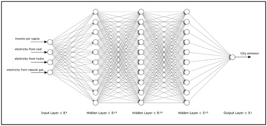
Figure 1.
Structure of the developed deep learning network.
As the first step, the deep learning network shown in Figure 1 is trained for optimizing the coefficients of the neurons of the network. A total of 70% of the available data are used for the training phase, while the remaining 30% of the data are employed as the test data to test the accuracy of the network. Nonlinear activation functions of the neurons are selected as hyperbolic tangent functions in the deep learning network. The presented deep learning network is developed in the Python programming language using the NumPy and Pandas numerical libraries and the MLPRegressor class from the SciKit-Learn (SKLearn) library [66,67,68]. The modelling results are given in the following Results and Discussion section.
4. Results and Discussion
The annual CO2 emission data of Turkey in the period of 1960–2020 are taken from the Our World in Data based on the Global Carbon Project website [69]. These CO2 data per year are plotted as in Figure 2 using the MatPlotLib library in Python [70].
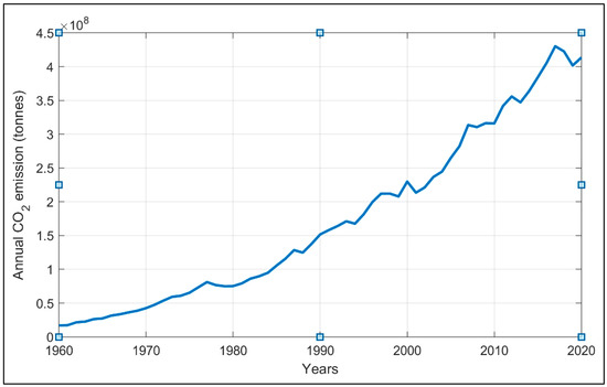
Figure 2.
The annual CO2 emission data of Turkey for the period of 1960–2020.
Firstly, Eviews software is utilized for the automatic ARIMAX modeling of the CO2 data dependent on the income per capita and the electricity consumption from hydroelectric, coal and natural gas resources. Structural break unit root tests are performed before the actual ARIMAX modeling phase. The results of the unit root tests are given in Table 1. The results of the automatic ARIMAX modeling are also summarized in Table 2.
Table 2.
ARIMAX modeling summary.
As the next step, the deep learning modelling is performed. A total of 70% of the available data are used as the training data and the remaining 30% of the data are used as the test data, which is a standard data split procedure. The train_test_split class of the SKLearn library is utilized for splitting the available data. The loss curve associated with the training phase of the developed loss curve is given in Figure 3.
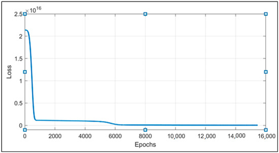
Figure 3.
The loss curve of the training phase of the deep learning network.
As can be seen from Figure 3, the training phase of the deep learning network is successfully completed, minimizing the loss value. As the next step, actual CO2 emission data, CO2 emission data obtained from the ARIMAX model and the CO2 emission data as the result of the developed deep learning network are plotted on the same axes in Figure 4. As can be observed from Figure 4, both the ARIMAX model and the deep learning network accurately model the annual CO2 emission data of Turkey in the 1960–2020 period employing the income per capita and the electricity consumption from the hydroelectric, coal and natural gas resources. In order to objectively assess the performance of the ARIMAX and deep learning models, figure of merit values, namely the coefficient of determination (R2), mean absolute error (MAE), mean absolute percentage error (MAPE) and the root mean square error (RMSE), are computed in Python using the formulas given in Equations (2)–(5) [71].
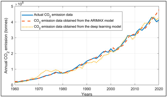
Figure 4.
The actual annual CO2 emission data and the CO2 emission data obtained from the ARIMAX and deep learning models.
In Equations (2)–(5), O represents the original data, N is the data obtained from the model and dim is the length of the time series. R2, MAE, MAPE and RMSE values for the ARIMAX and deep learning model results are calculated in the Python environment using the classes of the SKLearn.Metrics library, as presented in Table 3.
Table 3.
Performance parameters of the ARIMAX and the deep learning models.
As can be seen from Table 3, both ARIMAX and deep learning methods can be utilized to model the annual CO2 emission data dependent on the income per capita and electricity consumption from coal, hydroelectric and natural gas resources for Turkey in the period of 1960–2020. Considering the coefficient of determination and other performance parameters, it is observed that the deep learning model provides better performance compared to the ARIMAX model for modelling the annual CO2 emission data especially in the pandemic period of 2019–2020. It can be argued that either the ARIMAX model or the deep learning model can be used to model the annual CO2 emission data, providing insights for the estimation of the future emission data dependent on the income per capita and electricity usage, which would help to achieve the goals regarding the reduction in the carbon footprint according to the Paris Agreement.
5. Conclusions
Accurate modeling of annual CO2 emission data is of crucial importance considering the recently ratified Paris Agreement. Therefore, annual CO2 emission of Turkey for the period of 1960–2020 is modelled in this work. According to the original environmental Kuznets curve hypothesis, income per capita is the independent variable while CO2 emission is the dependent variable. In order to increase the performance of modelling the annual CO2 emission data, additional independent variables, namely the electricity consumption obtained from hydroelectric, coal and natural gas resources, are also included in this study. Two different approaches, ARIMAX and deep learning methods, are utilized for modelling the annual CO2 emission data dependent on income per capita and electricity consumption from the hydroelectric, coal and natural gas resources. Firstly, annual CO2 emission data and the independent variables are seasonally adjusted in Eviews software using the STL method. Structural break unit root tests are then applied for ensuring the stationarity of the data. Results of these tests are given in Table 1. Then, the ARIMAX model is developed in the EViews software. In the second part of the modeling phase, a deep learning network, consisting of three hidden layers employing multilayer perceptron neural networks, is developed in the Python programming language using the SciKit-Learn library. The available data are split as training and test data using the test_train_split class of Python, where 70% of the data are taken as the training data and the remaining 30% of the data are taken as the test data according to the standard procedure.
Actual annual CO2 emission data and CO2 emission obtained from the ARIMAX model and deep learning model are plotted on the same axes to visually inspect the performance of the developed ARIMAX and deep learning models. The plotted data indicate accurate modeling performance. In addition, the performance parameters of the ARIMAX and deep learning models, namely coefficient of determination (R2), mean absolute error (MAE), mean absolute percentage error (MAPE) and root mean square error (RMSE) values, are computed in the Python environment using the SciKit-Learn-Metrics library. The performance parameters show that both ARIMAX and deep learning models provide high-performance modelling of the annual CO2 emission data. Considering the coefficient of determination and other performance parameters, it is observed that the developed deep learning model provides higher accuracy compared to the ARIMAX model for modeling the annual CO2 emission data especially in the pandemic period of 2019–2020. Obtained results show that the annual CO2 emission data of Turkey can be modelled using both conventional ARIMAX and nonlinear deep learning methods, which would aid in forecasting CO2 emission data in order to make the required policy changes to achieve the aims of the Paris Agreement. In summary, the contributions of this study can be stated as follows. (i) The annual CO2 emission data are modelled utilizing explanatory variables, namely the electricity consumption obtained from the hydroelectric, coal and natural gas resources, to increase the accuracy, (ii) the conventional ARIMAX method is used to model the CO2 emission, (iii) a deep learning MLP network is also developed to model the CO2 emission, (iv) the results of the ARIMAX and deep learning MLP network are compared and (v) it is observed that both ARIMAX and the deep learning MLP network can be used to model the CO2 emission data; however, the deep learning model provides higher accuracy compared to the ARIMAX model.
Author Contributions
C.T.: Methodology, software, validation, writing—review and editing. D.S.Y.: Conceptualization, data curation, methodology, visualization, writing—original draft, writing—review and editing All authors have read and agreed to the published version of the manuscript.
Funding
This research received no external funding.
Institutional Review Board Statement
Not applicable.
Informed Consent Statement
Not applicable.
Data Availability Statement
Dataset available on request from the authors.
Conflicts of Interest
Author Cagatay Tuncsiper was employed by the company Centrade Fulfillment Services Ltd. The remaining author declares that the research was conducted in the absence of any commercial or financial relationships that could be construed as a potential conflict of interest.
References
- Kuznets, S. Economic growth and income inequality. Am. Econ. Rev. 1955, 45, 1–28. [Google Scholar]
- Grossman, G.M.; Krueger, A.B. Environmental Impacts of a North American Free Trade Agreement; Working Paper 3914 of the National Bureau of Economic Research; National Bureau of Economic Research: Cambridge, MA, USA, 1991; Volume 3, pp. 27–32. [Google Scholar]
- Benli, M. External debt burden—Economic growth nexus in Turkey. Soc. Sci. Res. J. 2020, 9, 107–116. [Google Scholar]
- Etokakpan, M.U.; Osundina, O.A.; Bekun, F.V.; Sarkodie, S.A. Rethinking electricity consumption and economic growth nexus in Turkey: Environmental pros and cons. Environ. Sci. Pollut. Res. 2020, 27, 39222–39240. [Google Scholar] [CrossRef]
- Report of the United Nations Conference on the Human Environment (the Stockholm Conference), 5–16 June 1972, Stockholm. Available online: http://undocs.org/en/A/CONF.48/14/Rev.1 (accessed on 1 March 2023).
- Report of the Brutland Commission, 30 October 1987, United Kingdom. Available online: https://sustainabledevelopment.un.org/content/documents/5987our-common-future.pdf (accessed on 2 March 2023).
- Adoption of the Kyoto Protocol to the United Nations Framework Convention on Climate Change, 1 December 1997, Kyoto, Japan. Available online: https://unfccc.int/decisions (accessed on 4 March 2023).
- Report of the Paris Agreement, 12 December 2015, Paris, France. Available online: https://unfccc.int/process-and-meetings/the-paris-agreement (accessed on 4 March 2023).
- Declaration of Intention of Turkey according to the Paris Agreement. Available online: https://www.mfa.gov.tr/paris-anlasmasi.tr.mfa (accessed on 1 March 2023).
- Lise, W. Decomposition of CO2 emissions over 1980–2003 in Turkey. Energy Policy 2006, 34, 1841–1852. [Google Scholar] [CrossRef]
- Hatzigeorgiou, E.; Polatidis, H.; Haralambopoulos, D. Energy CO2 Emissions for 1990–2020: A decomposition analysis for EU-25 and Greece. Energy Sources Part A 2010, 32, 1908–1917. [Google Scholar] [CrossRef]
- Carson, R.T.; Jeon, Y.; McCubbin, D.R. The relationship between air pollution emissions and income: US Data. Environ. Dev. Econ. 1997, 2, 433–450. [Google Scholar] [CrossRef]
- Zhang, M.; Mu, H.; Ning, Y. Accounting for energy-related CO2 emission in China 1991–2006. Energy Policy 2009, 37, 767–773. [Google Scholar] [CrossRef]
- Gunduz, H.I. Review of relationship between environmental pollution and income: Panel cointegration analysis and error correction model. Marmara Univ. J. Econ. Adm. Sci. 2014, 36, 409–423. [Google Scholar]
- Bruvoll, A.; Medin, H. Factors behind the environmental Kuznets curve: A decomposition of the changes in air pollution. Environ. Resour. Econ. 2003, 24, 27–48. [Google Scholar] [CrossRef]
- Deacon, R.T.; Norman, C.S. Does the environmental Kuznets curve describe how individual countries behave? Land Econ. 2006, 82, 291–315. [Google Scholar] [CrossRef]
- Burnett, J.W.; Bergstrom, J.C.; Wetzstein, M.E. Carbondioxide emissions and economic growth in the US. J. Policy Model. 2013, 35, 1014–1028. [Google Scholar] [CrossRef]
- Ang, C.B. Economic development, pollutant emissions and energy consumption in Malaysia. J. Policy Model. 2008, 30, 271–278. [Google Scholar] [CrossRef]
- Chang, C.C. A multivariate causality test of carbon dioxide emissions, energy consumption and economic growth in China. Appl. Energy 2010, 87, 3533–3537. [Google Scholar] [CrossRef]
- Magazzino, C. The relationship between CO2 emissions, energy consumption and economic growth in Italy. Int. J. Sustain. Energy 2016, 35, 844–857. [Google Scholar] [CrossRef]
- Mbarek, M.B.; Saidi, K.; Rahman, M.M. Renewable and non-renewable energy consumption, environmental degredation and economic growth in Tunusia. Qual. Quant. 2018, 52, 1105–1119. [Google Scholar] [CrossRef]
- Sarkodie, S.A.; Strezov, V. Effect of foreign direct investments, economic development and energy consumption on greenhouse gas emissions in developing countries. Sci. Total Environ. 2019, 646, 862–871. [Google Scholar] [CrossRef]
- Linh, D.H.; Lin, S.-M. CO2 emissions, energy consumption, economic growth and FDI in Vietnam. Manag. Glob. Transit. 2014, 12, 219–232. [Google Scholar]
- Grimes, P.; Jeffrey, K. Exporting the greenhouse: Foreign capital penetration and CO2 emissions 1980–1996. J. World Syst. Res. 2003, 2, 261–275. [Google Scholar] [CrossRef]
- Jorgenson, A.K. The effects of primary sector foreign investment on carbon dioxide emissions from agriculture production in less-developed countries 1980–99. Int. J. Comp. Sociol. 2007, 48, 29–42. [Google Scholar] [CrossRef]
- Yang, W.-P.; Yang, Y.; Xu, J. The impact of foreign trade and FDI on environmental pollution. China-USA Bus. Rev. 2008, 7, 1–11. [Google Scholar]
- Ahmed, K.; Shahbaz, M.; Qasim, A.; Long, W. The linkages between deforestation, energy and growth for environmental degradation in Pakistan. Ecol. Indic. 2015, 49, 95–103. [Google Scholar] [CrossRef]
- Al-Mulali, U.; Weng-Wai, C.; Sheau-Ting, L.; Mohammed, A.H. Investigating the environmental Kuznets curve (EKC) hypothesis by utilizing the ecological footprint as an indicator of environmental degradation. Ecol. Indic. 2015, 48, 315–323. [Google Scholar] [CrossRef]
- Apergis, N.; Ozturk, I. Testing environmental Kuznets curve hypothesis in Asian countries. Ecol. Indic. 2015, 52, 16–22. [Google Scholar] [CrossRef]
- Lau, L.S.; Choong, C.K.; Eng, Y.K. Investigation of the environmental Kuznets curve for carbon emissions in Malaysia: Do foreign direct investment and trade matter? Energy Policy 2014, 68, 490–497. [Google Scholar] [CrossRef]
- Jalil, A.; Mahmud, S.F. Environment Kuznets curve for CO2 emissions: A cointegration analysis for China. Energy Policy 2009, 37, 5167–5172. [Google Scholar] [CrossRef]
- Shahbaz, M.; Khraief, N.; Uddin, G.S.; Ozturk, I. Environmental Kuznets curve in an open economy: A bounds testing and causality analysis for Tunisia. Renew. Sustain. Energy Rev. 2014, 34, 325–336. [Google Scholar] [CrossRef]
- Shahbaz, M.; Dube, S.; Ozturk, I.; Jalil, A. Testing the environmental Kuznets curve hypothesis in Portugal. Int. J. Energy Econ. Policy 2015, 5, 475–481. [Google Scholar]
- Menyah, K.; Rufael, Y.W. CO2 emissions, nuclear energy, renewable energy and economic growth in the US. Energy Policy 2010, 38, 2911–2915. [Google Scholar] [CrossRef]
- Narayan, P.K.; Narayan, S. Carbon dioxide emissions and economic growth: Panel data evidence from developing countries. Energy Policy 2010, 38, 661–666. [Google Scholar] [CrossRef]
- Apergis, N.; Payne, J.E. Renewable energy consumption and growth in Eurasia. Energy Econ. 2010, 32, 1392–1397. [Google Scholar] [CrossRef]
- Tugcu, C.T.; Ozturk, I.; Aslan, A. Renewable and non-renewable energy consumption and economic growth relationship revisited: Evidence from G7 countries. Energy Econ. 2012, 34, 1942–1950. [Google Scholar] [CrossRef]
- Leitao, N.C. Economic growth, carbon dioxide emissions, renewable energy and globalization. Int. J. Energy Econ. Policy 2014, 4, 391–399. [Google Scholar]
- Apergis, N.; Danuletiu, D.C. Renewable energy and economic growth: Evidence from the sign of panel long-run causality. Int. J. Energy Econ. Policy 2014, 4, 578–587. [Google Scholar]
- Boluk, G.; Mert, M. Fossil & renewable energy consumption, GHGs (greenhouse gases) and economic growth: Evidence from a panel of EU (European Union) countries. Energy 2014, 74, 439–446. [Google Scholar]
- Ang, J.B. CO2 emissions, energy consumption, and output in France. Energy Policy 2007, 35, 4772–4778. [Google Scholar] [CrossRef]
- Kanjilal, K.; Ghosh, S. Environmental Kuznet’s curve for India: Evidence from tests for cointegration with unknown structural breaks. Energy Policy 2013, 56, 509–515. [Google Scholar] [CrossRef]
- Hamzacebi, C.; Karakurt, I. Forecasting the energy-related CO2 emissions of Turkey using a grey prediction model. Energy Sources Part A Recovery Util. Environ. Eff. 2015, 37, 1023–1031. [Google Scholar]
- Halicioglu, F. An econometric study of CO2 emissions, energy consumption, income and foreign trade in Turkey. Energy Policy 2009, 37, 1156–1164. [Google Scholar] [CrossRef]
- Mutafoglu, T.H. Foreign direct investment, pollution, and economic growth evidence from Turkey. J. Dev. Soc. 2012, 28, 281–297. [Google Scholar]
- Polat, M.A. The analysis of the relationship between foreign capital investments and CO2 emissions in Turkey through structural break tests. J. Int. Soc. Res. 2015, 8, 1127–1135. [Google Scholar]
- Balibey, M. Relationships among CO2 Emissions, economic growth and foreign direct investment and the environmental Kuznets curve hypothesis in Turkey. Int. J. Energy Econ. Policy 2015, 5, 1042–1049. [Google Scholar]
- Kizilkaya, O. The impact of economic growth and foreign direct investment on CO2 emissions: The case of Turkey. Turk. Econ. Rev. 2017, 4, 106–118. [Google Scholar]
- Saatci, M.; Dumrul, Y. The relationship between economic growth and environmental pollution: The estimation of environmental Kuznets curve with a cointegration analysis of structural breaks for Turkish economy. Erciyes Univ. J. Econ. Adm. Sci. 2011, 37, 65–86. [Google Scholar]
- Yavuz, N.C. CO2 emission, energy consumption, and economic growth for Turkey: Evidence from a cointegration test with a structural break. Energy Sources Part B Econ. Plan. Policy 2014, 9, 229–235. [Google Scholar] [CrossRef]
- Ozturk, I.; Acaravci, A. The long-run and causal analysis of energy, growth, openness and financial development on carbon emissions in Turkey. Energy Econ. 2013, 36, 262–267. [Google Scholar] [CrossRef]
- Shahbaz, M.; Ozturk, I.; Afza, T.; Ali, A. Revisiting the environmental Kuznets curve in a global economy. Renew. Sustain. Energy Rev. 2013, 25, 494–502. [Google Scholar] [CrossRef]
- Ocal, O.; Aslan, A. Renewable energy consumption-economic growth nexus in Turkey. Renew. Sustain. Energy Rev. 2013, 28, 494–499. [Google Scholar] [CrossRef]
- Altintas, H. The relationships between primary energy consumption, carbon dioxide emission and economic growth in Turkey: An analysis of cointegration and causality. Eskiseh. Osman. Univ. J. Econ. Adm. Sci. 2013, 8, 263–294. [Google Scholar]
- The Turkey Page of the Worldbank Website. Available online: https://data.worldbank.org/country/Turkiye (accessed on 1 March 2023).
- Cleveland, R.B.; Cleveland, W.S.; McRae, J.E.; Terpenning, I. STL: A seasonal-trend decomposition procedure based on loess. J. Off. Stat. 1990, 6, 3–73. [Google Scholar]
- Dickey, D.A.; Fuller, W.A. Distribution of the estimators for autoregressive time series with a unit root. J. Am. Stat. Assoc. 1979, 74, 427–431. [Google Scholar]
- Phillips, P.C.B.; Perron, P. Testing for a unit root in time series regression. Biometrika 1988, 75, 335–346. [Google Scholar] [CrossRef]
- Kwiatkowski, D.; Phillips, P.C.B.; Shmidt, P.; Shin, Y. Testing the null hypothesis of stationarity against the alternative of a unit root: How sure are we that economic time series have a unit root? J. Econom. 1992, 54, 159–178. [Google Scholar] [CrossRef]
- Yucesan, M. Sales forecast with YSA, ARIMA and ARIMAX methods: An application in the white goods sector. J. Bus. Res. 2018, 10, 689–706. [Google Scholar]
- Bierens, H.J. ARMAX model specification testing, with an application to unemployment in the Netherlands. J. Econom. 1987, 35, 161–190. [Google Scholar] [CrossRef]
- Arya, P.; Paul, R.K.; Kumar, A.; Singh, K.N.; Sivaramne, N.; Chaudhary, P. Predicting pest population using weather variables: An ARIMAX time series framework. Int. J. Agric. Stat. Sci. 2015, 11, 381–386. [Google Scholar]
- Sutthichaimethee, P.; Ariyasajjakorn, D. Forecasting energy consumption in short-term and long-term period by using ARIMAX model in the construction and materials sector in Thailand. J. Ecol. Eng. 2017, 18, 52–59. [Google Scholar] [CrossRef]
- LeCun, Y.; Bengio, Y.; Hinton, G. Deep learning. Nature 2015, 521, 436–444. [Google Scholar] [CrossRef]
- Murtagh, F. Multilayer perceptrons for classification and regression. Neurocomputing 1991, 2, 183–197. [Google Scholar] [CrossRef]
- van der Walt, S.; Colbert, S.C.; Varoquaux, G. The NumPy array: A structure for efficient numerical computation. Comput. Sci. Eng. 2011, 13, 22–30. [Google Scholar] [CrossRef]
- Kramer, O. SciKit-Learn in Machine Learning for Evolution Strategies; Springer: Berlin/Heidelberg, Germany, 2018. [Google Scholar]
- Lemenkova, P. Processing oceanographic data by python libraries NumPy, SciPy and Pandas. Aquat. Res. 2019, 2, 73–91. [Google Scholar] [CrossRef]
- The Turkey Page of the Our World in Data Based on the Global Carbon Project Website. Available online: https://ourworldindata.org/co2/country/turkey (accessed on 1 March 2023).
- Hunter, J.D. Matplotlib: A 2D graphics environment. Comput. Sci. Eng. 2007, 9, 90–95. [Google Scholar] [CrossRef]
- Mombeini, H.; Chamzini, A.Y. Modeling gold price via artificial neural network. J. Econ. Bus. Manag. 2015, 3, 699–703. [Google Scholar] [CrossRef][Green Version]


Disclaimer/Publisher’s Note: The statements, opinions and data contained in all publications are solely those of the individual author(s) and contributor(s) and not of MDPI and/or the editor(s). MDPI and/or the editor(s) disclaim responsibility for any injury to people or property resulting from any ideas, methods, instructions or products referred to in the content. |
© 2024 by the authors. Licensee MDPI, Basel, Switzerland. This article is an open access article distributed under the terms and conditions of the Creative Commons Attribution (CC BY) license (https://creativecommons.org/licenses/by/4.0/).