Abstract
Microgrids have been widely used due to their advantages, such as flexibility and cleanliness. This study adopts the hierarchical control method for microgrids containing multiple energy sources, i.e., photovoltaic (PV), wind, diesel, and storage, and carries out multi-objective optimization in the tertiary control, i.e., optimizing the economic cost, environmental cost, and the degree of energy utilization of microgrids. As the traditional multi-objective particle swarm algorithm is prone to local convergence, this study introduces variable inertia weight and learning factors to obtain a modified particle swarm algorithm, which is more advantageous in multi-objective optimization. Compared to the traditional particle swarm algorithm, the modified particle swarm algorithm increased the photovoltaic absorbed rate from 0.7724 to 0.8683 and the wind energy absorbed rate from 0.6064 to 0.7158 in one day, which resulted in an increase in energy utilization by 14.89%, and a reduction in financial environmental costs from RMB 135,870 to RMB 132,230. The simulation of the optimization effect of the conventional particle swarm algorithm and the modified particle swarm algorithm on the microgrid were carried out, respectively, in MATLAB, which verifies the advantage of the modified particle swarm algorithm on the optimization of microgrids. Then, the optimization results, i.e., the data of the power scheduling process of the four power sources, were made into a table and imported into the microgrid model in Simulink. The simulation results indicated that the microgrid was able to output stable voltage, current, and frequency. Finally, the changes in microgrids affected by the external environment were further investigated from the aspects of the market environment and natural environment. Moreover, we verified the presence of a contradiction between the optimization of the microgrid economy and environmental protection. Thus, microgrids need to adjust their optimization focus according to the natural conditions in which they are located.
1. Introduction
With the sustainable development of the world’s industry, the power system is also changing from fossil energy to clean energy, such as solar and wind [1]. As a result, hybrid microgrids have become an increasingly popular way of supplying electricity due to their reliability and operational efficiency [2]. Microgrids are the integration of distributed generations (DGs), energy storage devices, power electronic converters, and loads into a single system [3]. Microgrids are used in power grid applications for saving energy and reducing emissions, making environmental protection very favorable. The inputs of microgrids include photovoltaic, wind, and micro-diesel generators and other electrical energy, and the outputs comprise the voltage, frequency, and energy flows of microgrids. Its control requirements include system stability, response speed, and fault tolerance. Hierarchical control is the main method used for microgrids, and its control technology has become increasingly mature, with studies [4,5,6,7] adopting a hierarchical control structure for microgrids, primary control mainly using droop control to achieve stabilization of the microgrid output voltage and frequency, secondary control compensating for the drop caused by droop control, and the tertiary control carrying out the economic dispatch and energy management.
The study by [8] proposes a two-layer hierarchical optimization approach for a microgrid community energy management system in a smart grid environment. Ref. [9] proposes a hierarchical energy management system to address the issues of energy trading, network interconnection, and the intermittency of renewable energy sources. Ref. [10] presents a hierarchical control scheme for islanded AC microgrids, which has droop control and centralized extended optimal tidal current control. Ref. [11] proposes a hierarchical control scheme utilizing a new control loop to control reactive power references through a nonlinear fuzzy logic controller. From the above literature studies, it can be seen that the hierarchical control method and its application for microgrids are very mature, so the microgrid in this study also adopts a hierarchical control structure.
Due to the lack of optimal configuration and optimal operation, the implementation of microgrids often lacks economic and environmental benefits. Based on this, microgrids need to rapidly coordinate the control of source–storage–load with intraday or real-time adjustments at the coordinated control layer and local control layer to ensure stable operation and maximize clean energy utilization [12]. Therefore, the entire microgrid system must be analyzed and designed to operate in a stable region [13]. Numerous studies used multi-objective optimization algorithms to optimize the operation of microgrids in their tertiary control [14,15,16,17]. Ref. [18] proposed a self-optimizing droop control strategy based on optimal operating conditions to improve the overall operational performance of the system. Ref. [19] proposed a multi-objective selection optimization method to optimize the combined economic–environmental benefits of grid-connected microgrids.
In the study by [20], a multi-objective microgrid energy optimization model was developed using the beetle antenna search algorithm to optimize energy management and scheduling for microgrids of renewable energy, conventional energy, and energy storage systems. Ref. [21] proposed a multi-objective particle swarm optimization algorithm for archive update mechanism based on nearest neighbour approach. Ref. [22] proposed a new multi-objective rectification strategy to improve the load frequency control of islanded microgrids. Ref. [23] introduced a new critical load vector microgrid optimization design methodology to find the desired balance between microgrid power availability, net present value cost, and power efficiency. Ref. [24] proposed a two-step multi-objective hybrid battery storage system management approach by hybridizing two battery storage systems for shipboard microgrids. From all these studies, it can be seen that there are various multi-objective optimization methods for microgrids; however, the objectives of their concern are different. In this study, we optimize the economic cost, environmental cost, and the degree of energy utilization, and a particle swarm algorithm with a stronger global search capability and faster convergence is used.
There are also some related research studies about the particle swarm algorithm. In relation to this, ref. [25] established a multi-objective optimization mathematical model based on the comprehensive consideration of economy, environment, and battery cycle power in the microgrid scheduling process. Ref. [26] proposed a meta-heuristic hybrid algorithm, i.e., a hybrid frog leaping algorithm (SFLA) and particle swarm optimization algorithm (PSO), for solving a multi-objective optimal power flow while considering multi-fuel constraints. Ref. [27] explored the use of the integrated learning particle swarm optimization algorithm and differential evolutionary algorithm in a fuzzy frame to solve the optimal active scheduling (OAPD) problem. Based on the fuzzy mathematical theory, a fuzzy multi-objective optimization model with associated constraints minimizes the total economic cost and network losses of microgrids [28]. Ref. [29] considers the microgrid power output and carbon emission constraints in the grid-connected mode. The optimal model to reduce carbon emission cost and optimize economic operation is proposed.
Particle global optimization and external file maintenance strategies are designed to improve the load distribution capability of traditional multi-objective particle swarm optimization [30], which also optimizes the decision maker’s preference for the objective through a fuzzy decision-making scheme. Ref. [31] established a multi-objective hierarchical optimization model based on considering the comprehensive impact of DG access and the importance of loads, and taking the optimal microgrid operation economics as the objective function.
The above articles show that the particle swarm algorithm utilizes its full advantage in microgrid optimization, and has been widely applied to the multi-objective optimization of microgrids. However, the traditional particle swarm algorithm still has some deficiencies. In the conventional particle swarm algorithm, the values of inertia weight and the learning factors and are fixed, which leads to the traditional particle swarm addressing not being comprehensive. Thus, it is easy to fall into the local optimal problem. However, this study introduces the variable inertia weight and the learning factors to improve the particle swarm algorithm in multi-objective optimization. Compared to the above studies in [26,27], the modified PSO is more sensitive to population initialization and is also prone to produce locally optimal solutions when the initial population distribution greatly varies. The modified particle swarm algorithm is more advantageous in multi-objective optimization and can produce a better optimization effect for microgrids. The main contributions of this study are as follows:
- (1)
- The introduction of variable inertia weight and learning factors to improve the particle swarm algorithm for the uncertain system scenarios in microgrids due to the stochastic nature of power generation and load demand. Its operation resulted in better optimization of the tertiary control of the microgrid, reduced energy losses, increased utilization of renewable energy, and enabled the microgrid to operate in a more economical manner.
- (2)
- The microgrid model is built in Simulink for simulations, and the microgrid is controlled by hierarchical control, which contains primary control and secondary control to realize the stable operation of the microgrid. Then, the data of the power scheduling process of the modified particle swarm algorithm are imported into the microgrid model in Simulink, and the results verify that the modified particle swarm algorithm can be applied to the microgrid.
- (3)
- Starting from the market environment and the natural environment, respectively, the changes in the microgrids affected by the external environment are further studied. It is verified that there is a contradiction between the optimization of microgrid economy and environmental protection. Moreover, microgrids need to adjust their optimization focus according to the natural conditions in order to obtain a better operation scheme.
2. Hierarchical Control of Microgrids
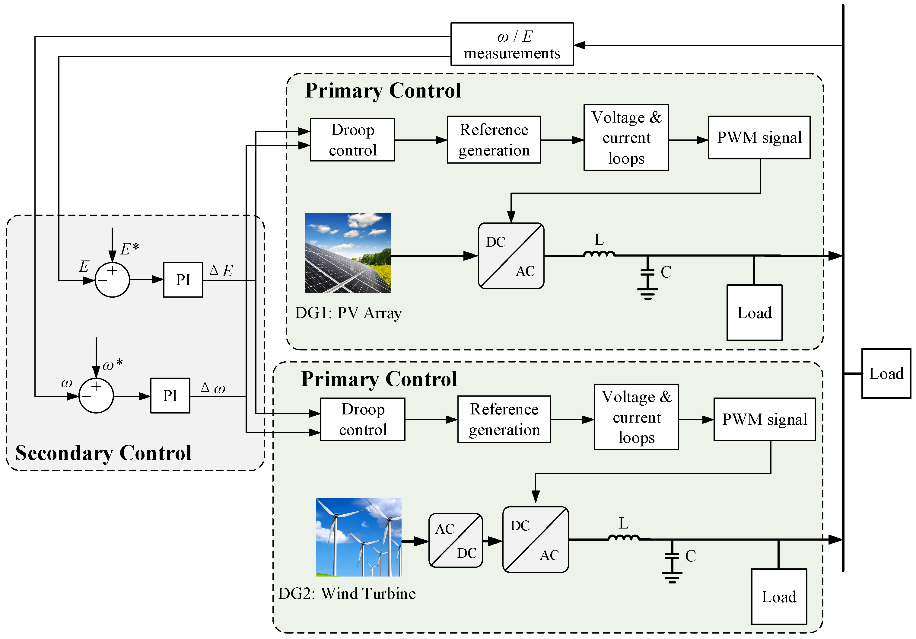
The hierarchical control structure of the microgrid in this study has two layers, and its control structure is shown in Figure 1, where L and C are used to filter the output voltage of the DG, and are the frequency and amplitude of the microgrid output voltage obtained from the measurements, and and are the frequency reference value and amplitude reference value of the microgrid output voltage, respectively. The primary control includes the droop controller, the reference voltage generation part, the voltage–current double closed-loop control, and a pulse width modulation (PWM) signal generator. The secondary control makes a difference between the frequency and amplitude of the microgrid output voltage and its set reference value, and then outputs the frequency adjustment amount and amplitude adjustment amount through the PI controller and acts in the droop control, and finally changes the PWM signal to regulate the power converters of each DG of the microgrid so that it outputs stable voltage and current.
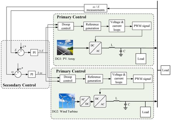
Figure 1.
Hierarchical control structure of microgrids.
2.1. Primary Control
Primary control is mainly concerned with the stability of the local control and the drive signal of the power converter. Droop control is commonly used in primary control, and the droop control strategy has a similar principle to the primary frequency regulation of traditional generators. The control principle outlines the process when the active and reactive power of the microgrid change, the microgrid adjusts the frequency and amplitude of its output voltage according to the P-f and Q-U droop relationship. The equations used in the regulation process are as follows:
where is the output frequency of the microgrid, is the output voltage of the microgrid; and are the rated frequency and rated voltage of the microgrid, respectively; m and n are the droop control coefficients; and are the active and reactive power of the microgrid, respectively; and and are the rated active and rated reactive power of the microgrid, respectively.
2.2. Secondary Control
In order to compensate for the decrease in frequency and amplitude caused by the primary control, the secondary control method is usually used to restore them to their rated values. As shown in Figure 1, the secondary control first obtains the real-time frequency and voltage magnitude of the microgrid output voltage through a measuring device and compares the real-time values with the reference values. Furthermore, the deviation is compensated by a PI controller, which ultimately brings the frequency and magnitude of the microgrid output voltage close to the set reference values. The mathematical expression of the control method is
where and denote the proportional and integral parameters of the PI controller for frequency C. In addition, and denote the proportional and integral parameters of the PI C amplitude compensation in the secondary control; and are the output frequency and voltage amplitude of microgrids; and are reference values of frequency and voltage amplitude, respectively; and and are the regulation values of the frequency and voltage amplitude of the controller output, respectively.
3. Tertiary Control Optimization Methods: Particle Swarm Algorithms
The multi-objective scheduling scheme of the wind–photovoltaic (PV)–diesel–storage microgrid system studied in this paper considers three indicators, namely its economic cost, energy utilization degree, and environmental cost in the islanded state. A multi-objective microgrid model containing PV generators, wind turbines, diesel engines, and storage batteries is established.
3.1. Construction of Microgrid System Scheduling Model Based on Particle Swarm Algorithm
3.1.1. Wind–PV–Diesel–Storage Microgrid Contribution Model of Each Component
According to the characteristics of each component’s output, the output model is analyzed as follows:
- The power of the wind turbine is determined by the wind speed of the region where it is located and the rated power of the generator. The output model expression is as follows:where is the rated power of the wind turbine, is the cut-in wind speed, and is the cut-out wind speed. When the wind speed is less than the cut-in wind speed or greater than the cut-out wind speed, the turbine power will be 0. When the wind speed is between the rated wind speed and the cut-out wind speed, the turbine power will keep the rated power unchanged.
- The power of PV is mainly related to the light intensity and ambient temperature in its region, and the expression of the output model is as follows:where is the output power measured under rated conditions; is the irradiation intensity under rated conditions; is the irradiation intensity at a certain time; is the reference temperature, taking 25 °C; is the surface temperature of the solar panel at a certain time; and k is the power temperature coefficient. From Equation (6), it can be seen that the power generation of solar cells as well as light intensity and ambient temperature are positively correlated.
- Diesel generator output is more stable than that of wind and PV, and it is mainly used as a reliable guarantee in power generation scheduling to maintain normal operation of the microgrid in the case of insufficient new energy output. Its operating power can be kept constant or adjusted between the maximum and minimum power according to the load change to meet the demand. The diesel engine output model is expressed as follows:where is the fuel absorption rate, is the rated power of the diesel engine, is the actual output power of the diesel engine, and and are the correlation coefficients of the diesel generator fuel absorption curve. Diesel generator fuel absorption can be inverted through the diesel generator power generation.
- Wind power generation units and PV power generation units are greatly affected by weather and climate, resulting in uncertainty in their power output, which can easily have an impact on the power grid and deteriorate its power quality. Therefore, the energy storage unit is indispensable for the microgrid. Battery is currently the most mature technology of a battery energy storage technology, with high energy density, stable energy supply, and high cycle efficiency [32]. In this paper, the battery is used as an energy storage device. Its output is related to the battery capacity and deep discharge, which can discharge when the load is not met, charge and store electric energy when the power exceeds the load, and play the role of peak cutting and valley filling. The model is as follows:where is the battery capacity, and are the charging and discharging powers, respectively, and are the charging and discharging efficiencies, S is the rated capacity of the battery, and is the time step.
3.1.2. Objective Function
Microgrid optimization scheduling needs to consider a number of indicators in order to achieve a more optimal performance while meeting the demand load. There are three optimization indexes measured in this paper. One of which is the economic cost, the second is the degree of energy utilization, and the third is the environmental cost. The main objective of this paper is to achieve the goal of minimizing the combination of economic cost, wind, and PV waste rate and environmental pollution by rationally allocating the current generation capacity of each generation unit. The overall objective function is as follows:
where Fnc is the economic cost, which mainly takes into account the generation cost, maintenance cost, battery deep charging/discharging cost, and abandonment/shortage cost of each generation unit; the calculation formula is as follows:
where UE is the degree of energy utilization, which is mainly used to measure the degree of utilization of clean energy by microgrids, and its expression is a linear comprehensive function of the respective absorption rates of wind and PV power generation as follows:
where and are the PV absorption rate and wind absorption rate, respectively, and their values are the ratios of the total amount of generation utilized by the current dispatch scheme to the total amount of generation predicted to be available on that day, both of which are in the range of [0, 1]. Due to the target optimization seeking the minimum value, the degree of energy utilization indicators in the processing of 2 minus the sum of the wind and PV absorption ratio was chosen in order to ensure that the results were positive at the same time, so that the value of the degree of energy utilization became negatively correlated, that is, the smaller the result of the numerical value of the wind and PV integrated rate of absorption of the higher, the higher the degree of energy utilization. The value range of the final data is [0, 2].
Green is the cost of environmental protection, which identifies the amount of pollutant gases generated during the diesel power generation process, which is calculated as the cost of treating the main harmful gases (including CO2, SO2, and NOx) generated by the diesel engine per unit of power generation, with the following expression:
where , , and are the governance costs of CO2, SO2 and NOx, respectively, which are calculated as follows:
where is the cost of treating each kilogram of pollutant, k in the subscript represents three different pollutant gases, and represents the pollutant emission when the output power of diesel engine is P.
Since optimal scheduling needs to be solved using intelligent algorithms, measuring the three indicators requires extending the exploration space of the algorithms to three dimensions—which is difficult in model building—while the convergence speed of the algorithms may slow down considerably—which is not conducive to algorithmic optimization. A simplified mindset was adopted by combining the environmental and economic aspects into a single indicator—financial environmental cost (FEC).
In the study by Linjing Hu et al., ref. [33] considers wind/PV stability with two performance indicators: loss of power supply probability (LPSP) and energy waste rate (EWR). In order to improve the convergence speed, the two metrics are combined into a single metric LE that is balanced with a custom parameter α, which is shown as follows:
This section draws on this methodology by similarly treating economic cost and environmental cost by summing the costs incurred by both and introducing customized parameters for balancing, with the following expressions:
The parameters can be changed to adjust the weight of the two components and modify the focus of the microgrid optimization scheme according to the overall needs of the grid. Therefore, the multi-objective expression of the final system is as follows:
3.1.3. Restrictive Condition
- 1.
- Constraint of Generator Set
In terms of the actual configuration of the microgrid, it is necessary to consider the capacity of each power generation component to ensure that the capacity of each PV generator set is reasonable. In the case of being able to satisfy the load, the scale of the configured equipment should not be too large to save space and economic costs.
Constraints on PV unit output:
Constraints on wind turbine output:
Constraints on diesel generator sets:
- 2.
- Battery Operation Constraints
The energy storage unit has the role of peak shaving and valley filling. When the power grid generates excess power in the low valley, the energy storage unit stores energy. When the power grid generates insufficient power in the high peak, the energy storage device releases energy, which effectively improves the economy of the system operation, reduces the waste of energy, and also regulates the power fluctuation of the load. In this paper, the battery is used as the energy storage device, and its working state has two kinds of charging and discharging. The maximum charging capacity is expressed as a negative number, and the maximum discharging capacity is expressed as a positive number.
The output constraints are as follows:
The capacity constraints are as follows:
where is the current battery capacity, is the maximum capacity of battery deep discharge, and is the maximum capacity of battery charging.
- 3.
- Generation Margin Constraints
The generation margin is the sum of the difference between the dispatched generation and the expected load, and its calculation expression is as follows:
where is the microgrid dispatch generation at moment i, is the expected load value at moment i, and the two are accumulated to obtain the difference between the dispatch generation and the overall expected load in a day.
In order to ensure the reliability of the grid generation, it is necessary to limit the difference between the generation and the expected load not to exceed a certain limit, with the following constraints:
3.2. Research and Improvement of Particle Swarm Algorithm
In the conventional particle swarm algorithm, the values of inertia weight and learning factors , are fixed, which leads to the problem that the traditional particle swarm addressing is not comprehensive and easily falls into the local optimal solution. In order to improve this defect and make the addressing range more extensive, it is necessary to introduce parameter values that change with the increase in the number of iterations, which gives rise to the improved particle swarm algorithm. The basic goal to be achieved by the parameter changes is to make the particle swarm tend to learn autonomously in the early iteration, thus expanding the range of movement of the particle swarm, and to make the particle swarm tend to learn socially in the late iteration, thus accelerating the convergence speed and obtaining the global relative optimal solution.
There are many ways and methods of parameter change guided by this concept, such as linear change and adaptive change. The former mainly realizes the parameter change by presetting the initial and final values of the parameters, and then specifying the linear function that changes with the number of iterations, while the latter needs to consider the current particle’s fitness and the average fitness, and continuously corrects the parameters through screening. In this paper, the linearly varying inertia weight and learning factors are used, and are formulated as follows:
where is the number of iterations; is the maximum number of iterations; , , and are the initial values of inertia weight, self-learning factor, and community learning factor, respectively; and , , and are their final values, respectively.
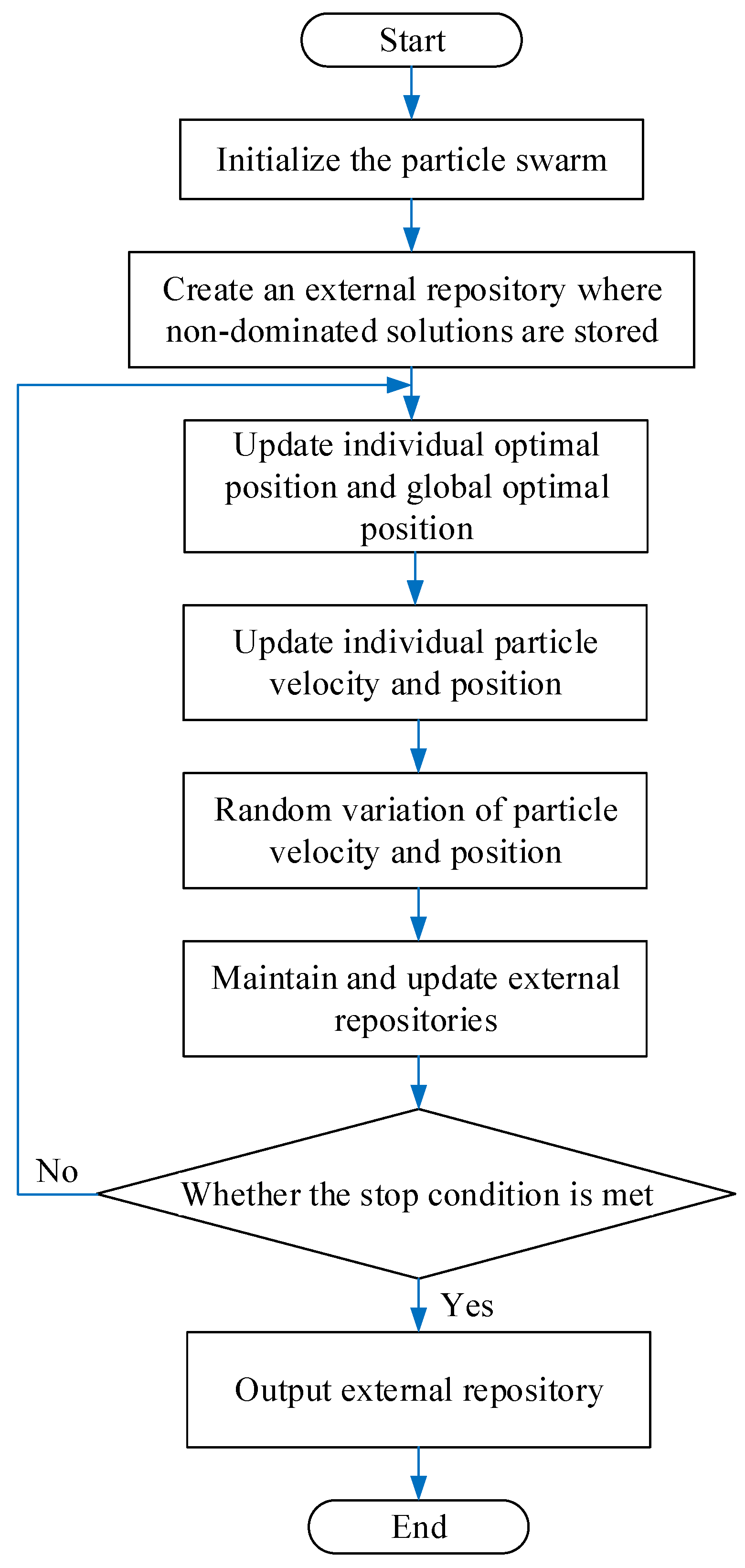
The modified particle swarm algorithm sets up an external repository in order to filter and store the particles that meet the requirements. The particles in the repository determine the particle swarm moving state, and the addition and deletion of particles in the repository are accomplished by the adaptive grid method. The current optimal solution of the swarm is selected by roulette. The search range is divided into grids, each grid is numbered, and the grid to which each particle belongs is labeled by the serial number, and finally the non-dominated solution of the particle is randomly selected from the grid to determine the current optimal position of the particle. Each particle is also randomly mutated during the iteration process, floating up and down the current range to increase the diversity of particles. The final repository holds a series of nondominated solutions as output data, and the final result is subsequently rationalized by selecting the final result based on a trade-off formula determined by the prioritization of the microgrid objectives. The flowchart of the modified particle swarm algorithm is given below (Figure 2).
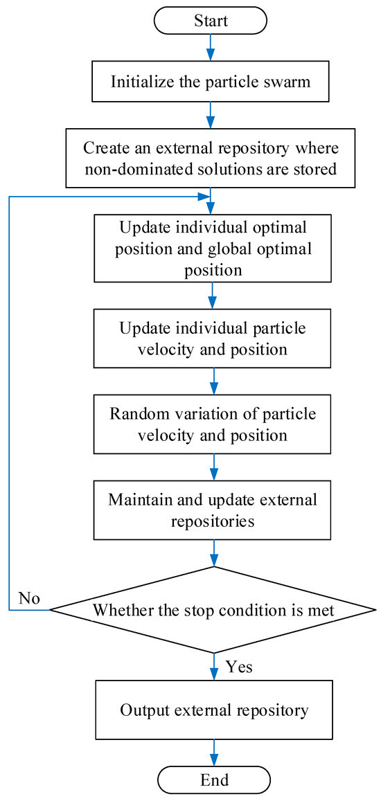
Figure 2.
Modified particle swarm algorithm flowchart.
4. Simulation Results and Discussions
4.1. Particle Swarm Algorithm Simulation
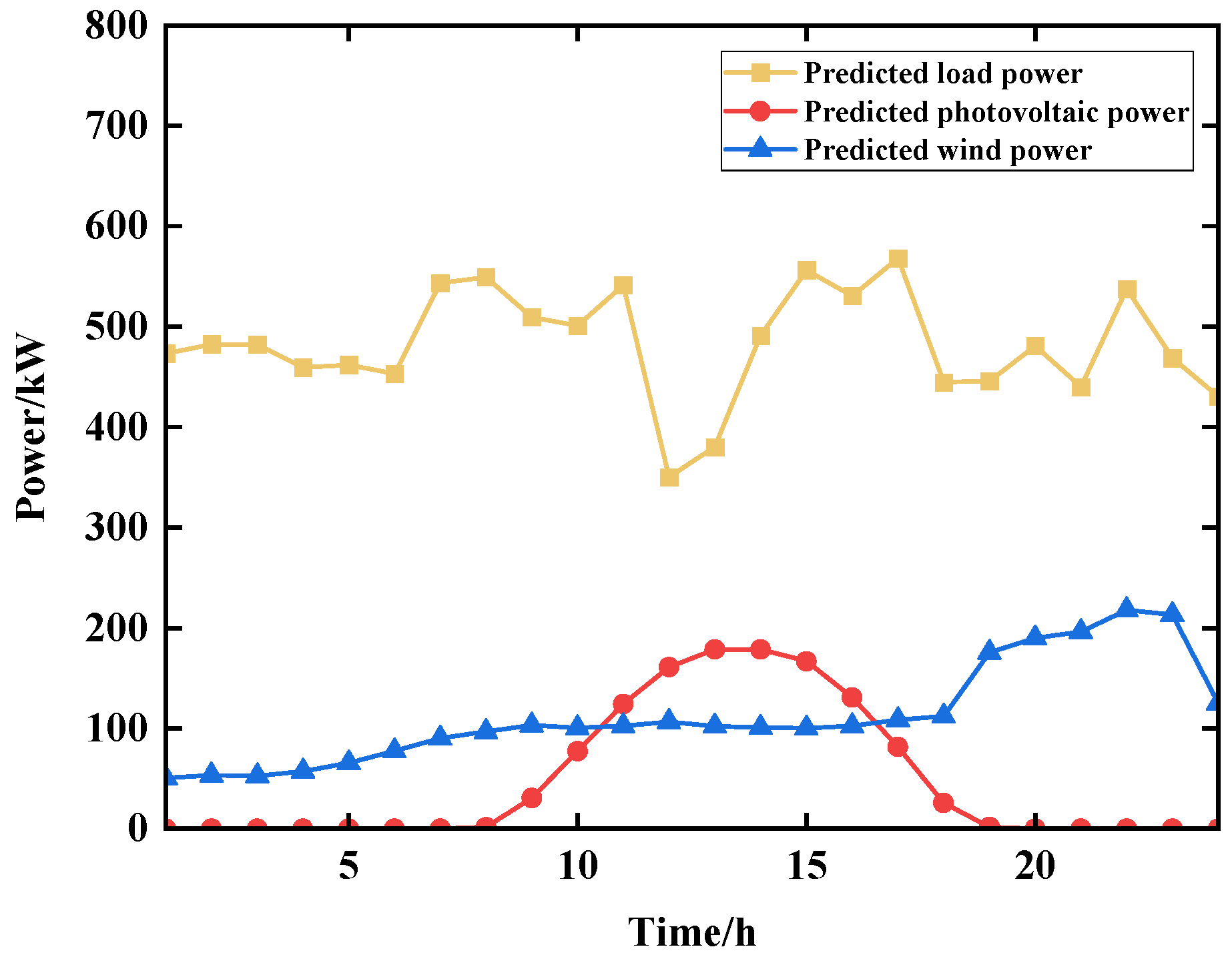
In this study, the Pareto optimal solution theory is adopted to solve the multi-objective optimal scheduling problem of microgrids; the traditional particle swarm and improved particle swarm algorithms are used as the intelligent optimization algorithms; and the data of a power grid in East China are used as the simulation data. The wind power, PV, and load prediction curves in this region are shown in Figure 3. The configuration of the diesel engine unit generates power in the range of 100–400 kW, the maximum charging power of the energy storage battery pack is −200 kW, and the maximum discharging power is 250 kW. The predicted load demand is in the range of 300–600 kW. The whole microgrid can meet the predicted load.

Figure 3.
East China Power Station predicted curve.
A series of nondominated solutions obtained after addressing of particle swarm algorithm is used to obtain the final scheduling result by weighted summation method. All the objective values are normalized and assigned according to the weight. Finally, the particle with the smallest combined value after summation is taken as the optimal solution, i.e., a compromise solution is searched for as the final scheduling solution. The formula is as follows:
where , , and are the weight of each objective value; , , and are the corresponding maxima in the set of non-dominated solutions for each objective value, respectively.
4.2. Traditional Particle Swarm Algorithm Simulation
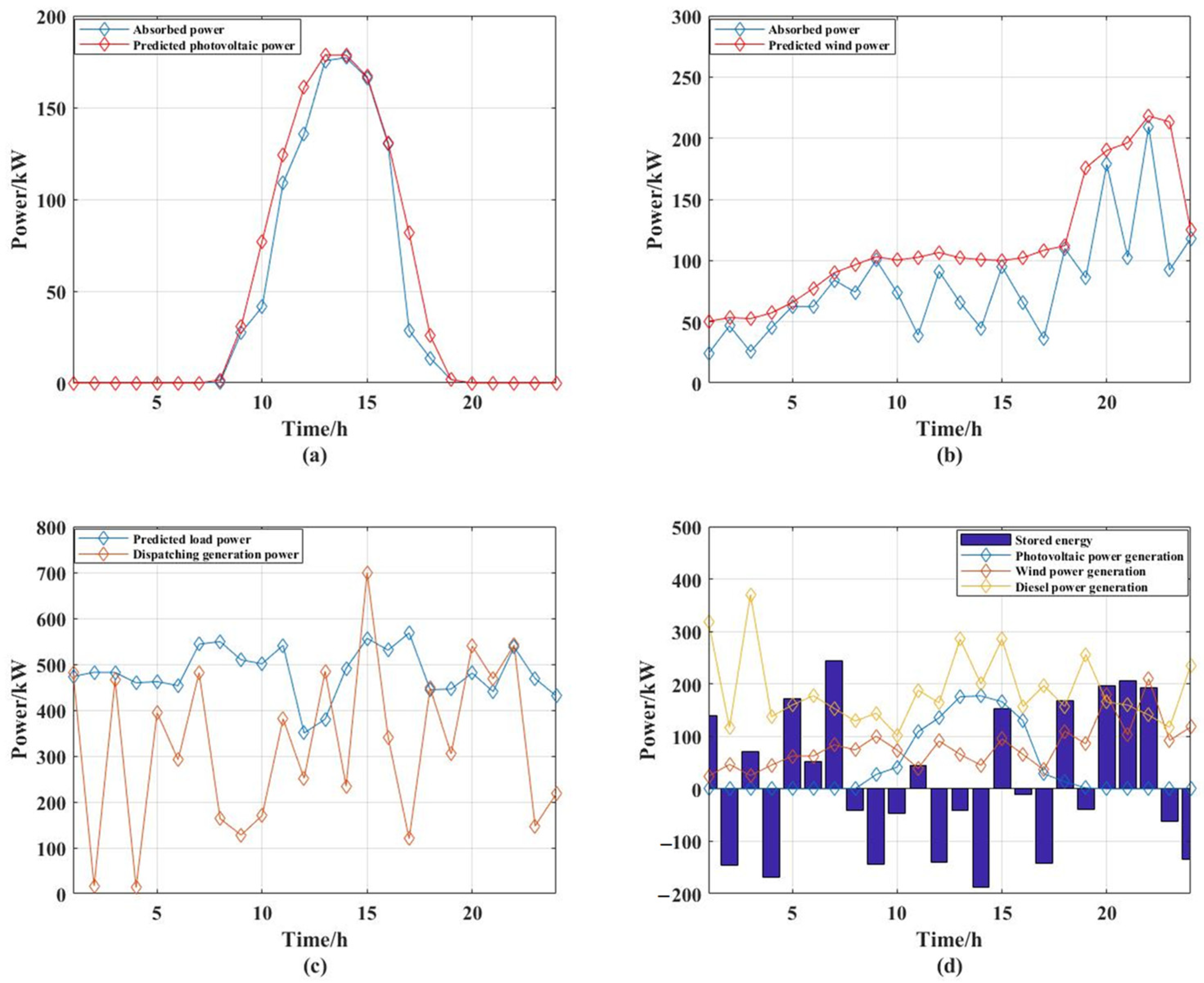
The particle swarm algorithm program is built according to the traditional particle swarm characteristics and is implemented in Matlab 2020b. Based on its standard value range, the parameter values are selected after reasonable testing. The final inertia weight is set to 0.5, the self-learning factor is set to 0.1, the community learning factor is set to 0.2, and the number of iterations is 100. The execution time is 30.009 s. The simulation results are shown in Figure 4.
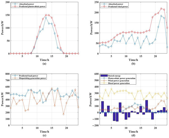
Figure 4.
Traditional particle swarm simulation results: (a) PV generation output; (b) wind generation output; (c) dispatching generation and predicted load; and (d) each component dispatching power generation.
The values of the indicators: the degree of energy utilization is 0.7452; the rate of PV absorption is 0.6578; and the rate of wind absorption is 0.5970; the financial environmental cost is RMB 135,870; the economic cost is RMB 135,380; and the environmental cost is RMB 491.569.
The large values obtained for the energy utilization degree indicator indicate that the PV and wind absorption rates are not excellent. Figure 4a,b show that the dispatch generation of wind and PV outlets is not a very good fit to the predicted capacity.
As can be seen from Figure 4c, the dispatched generation is lower than the predicted load and the gap is larger before 11:00, and gradually approaches the predicted load after 13:00, but there are still some moments when the generation is too low.
From Figure 4d, it can be seen that the diesel engines are more powerful throughout the whole process. Moreover, PV and wind power generation basically follow the law of unit power, but energy storage charging and discharging is more disordered, and it does not play a good role in shaving peaks and filling valleys.
4.3. Modified Particle Swarm Algorithm Simulation
The initial and final values of the inertia weight of the modified particle swarm algorithm are set to 0.9 and 0.2, respectively, and the larger initial value in the early stage facilitates the global search, while the weight gradually decrease as the number of iterations increases, which is convenient for the convergence of the particle swarm. The initial and final values of the self-learning factor are 1.2 and 0.02, respectively. The initial and final values of the community learning factor are 0.01 and 1.2, respectively. The execution time is 27.882 s. The larger self-learning factor and smaller community learning factor in the early stage can reduce the external influences on the particles, which is conducive to the wide range of activities within the feasible range and the global search; the smaller self-learning factor and larger community learning factor in the later stage can increase the particle’s ability to follow the global optimum, which is more conducive to the particle localization of the optimal solution. The simulation results are shown in Figure 5.
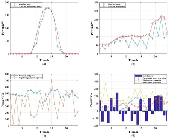
Figure 5.
Modified particle swarm simulation results: (a) PV generation output; (b) wind generation output; (c) dispatching generation and predicted load; and (d) each component dispatching power generation.
The values of the indicators: energy utilization degree is 0.4159; the PV absorption rate is 0.8683; wind absorption rate is 0.7158; the financial environmental cost is RMB 132,230; the economic cost is RMB 131,690; the environmental cost is RMB 533.454.
The value of energy utilization degree is low, indicating that the performance is better. It can also be seen from Figure 5a,b that the fit between the dispatched generation and the predicted generation is very high, which is significantly better than the traditional particle swarm scheduling results. It can be seen that the diesel power generation in the mid-day PV power generation out of the more significant decline, PV power generation is concentrated in the 9:00–17:00 of the mid-day moment, and wind power generation is concentrated in the 18:00–23:00 of the sunset and nighttime moments: the two form a staggered peak complementary effect. Figure 5c,d show the energy storage battery in the PV and wind power generation peak charging and reducing the power generation. With the diesel engine working, there is a better peak that enables the valley to be filled, stabilizing the microgrid power supply.
4.4. Comparative Analysis of Conventional Particle Swarm Algorithm and Modified Particle Swarm Algorithm Simulation
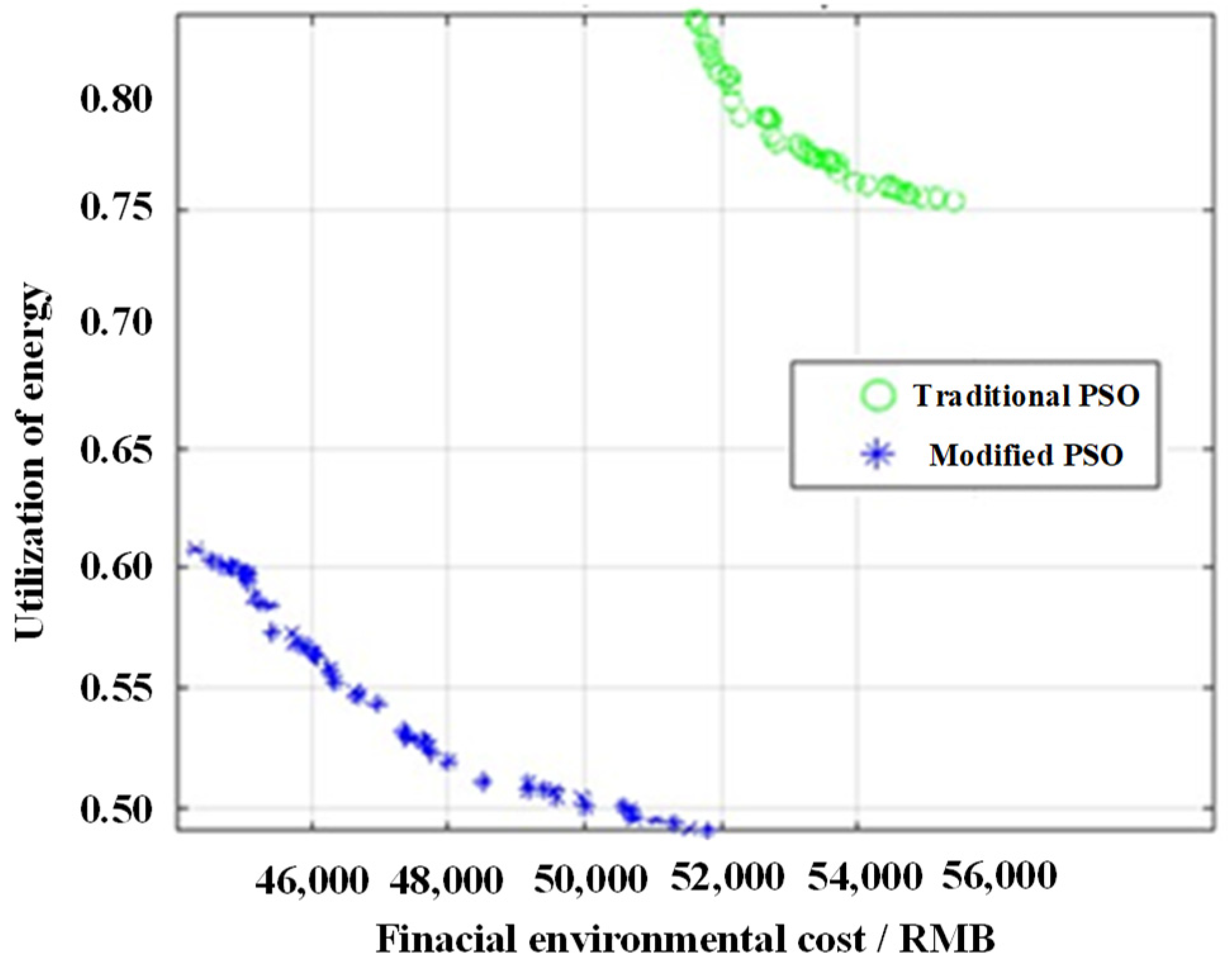
The respective Pareto frontier surfaces of the conventional particle swarm and the modified particle swarm algorithm can be shown by the particle positions in the external repository. As shown in Figure 6, it can be seen that the frontier surface of the modified particle swarm algorithm was advanced in comparison to the conventional particle swarm by the two objective terms stipulated in Equation (16). Moreover, the environmental economy and the degree of energy utilization were optimized, so the solution set of the modified particle swarm algorithm dominates over the solution set of the traditional particle swarm algorithm. This means that the modified particle swarm algorithm finds a more excellent scheduling scheme.
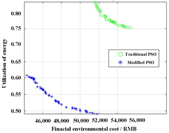
Figure 6.
Pareto frontier comparison between conventional particle swarm algorithm and modified particle swarm algorithm.
At the same time, it can be clearly seen that the number of particles in the storage library of the modified particle swarm algorithm is large and widely distributed. Compared to the conventional particle swarm that is overly centralized and has a small number of particles, the modified particle swarm can utilize the space of the external storage library more efficiently, reduce the waste, and reduce the possibility of local convergence. The modified particle swarm algorithm has a higher convergence in the multimodal problems with a convergence rate from 33.009 s to 27.882 s, as well as simulation results yielding a better global optimal solution than the traditional PSO.
The modified particle swarm algorithm has better global search capability. Its convergence speed varies depending on the complexity of the problem and the number of optimization objectives, and the parameter settings are also crucial to its performance and convergence characteristics. The modified particle swarm algorithm can improve its convergence accuracy.
In order to compare the modified particle swarm algorithm more rigorously to the conventional particle swarm algorithm, the two algorithms are run 100 times under the same conditions. The number of each iteration is 100, and the average and optimal values of the final scheduling results are compared in the following Table 1. Moreover, the total margin of power generation is also added to further measure the performance of scheduling scheme.

Table 1.
Comparison of the results of the modified particle swarm algorithm with the conventional particle swarm algorithm.
As can be seen from the data in Table 1, the time used for 100 runs of the modified particle swarm is longer, indicating that its convergence speed is slower than that of the conventional particle swarm. However, both the average value and the optimal value of the modified particle swarm optimization objective are better than the conventional particle swarm algorithm in terms of energy utilization and economic and environmental protection. In terms of the average value, the value of economic and environmental protection is 29.5% lower than that of the conventional particle swarm. The modified particle swarm also outperforms the conventional particle swarm algorithm in terms of the difference between the dispatched generation and the predicted load. The absolute value of the total generation margin is reduced by 21.1% compared to the conventional particle swarm, which makes the power supply capacity of the microgrid more reliable.
In summary, the modified particle swarm with variable inertia weight and variable learning factors can address systems more widely, break the limitation of conventional particle swarm that is easy to converge on the local optimal solution, improve the utilization rate of the microgrid for wind and PV generation, and reduce the operating cost of the microgrid, which leads to the improved performance of the final scheduling scheme in many aspects.
4.5. Simulation of Results of Modified Particle Swarm Algorithm Runs in Simulink
The scheduling results of wind, PV, diesel, and energy storage components are saved, and then a microgrid model is constructed in Simulink, where four DGs represent PV, wind, diesel, and energy storage components, respectively. Further, the particle swarm algorithm’s process of regulating the power of each component is added to each DG, and the 24 h power regulation process is simulated as 48 s, i.e., every two seconds represents an hour, and the simulation results are described below.
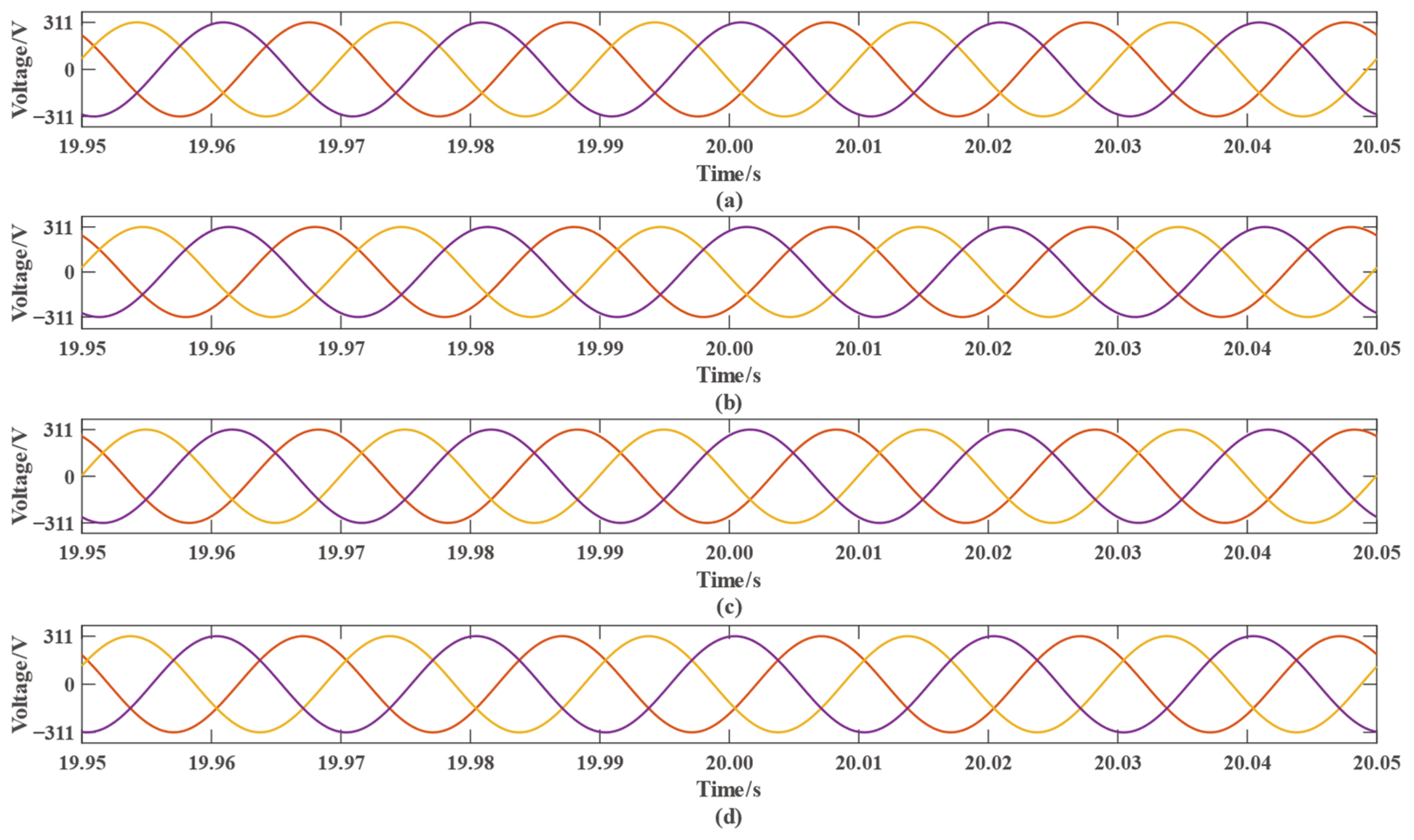
Figure 7 shows the voltages of each component of the microgrid within the period from 19.95 s to 20.05 s. Figure 7a–d represent the voltages of the PV, wind, diesel, and storage parts, respectively. The orange, purple, and yellow lines in Figure 7a–d represent the output three-phase voltage, respectively. It can be seen that the output voltages of each component in this time period are relatively standard three-phase sinusoidal waves, and the amplitudes are all stabilized at 311 V.
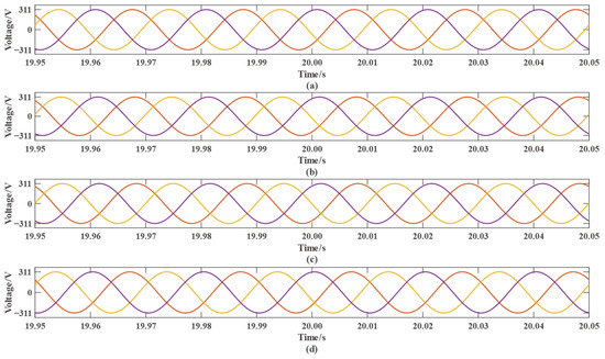
Figure 7.
Output voltage of the microgrid at a certain time period: (a) output voltage of PV power generation; (b) output voltage of wind power generation; (c) output voltage of diesel power generation; and (d) output voltage of the energy storage section.
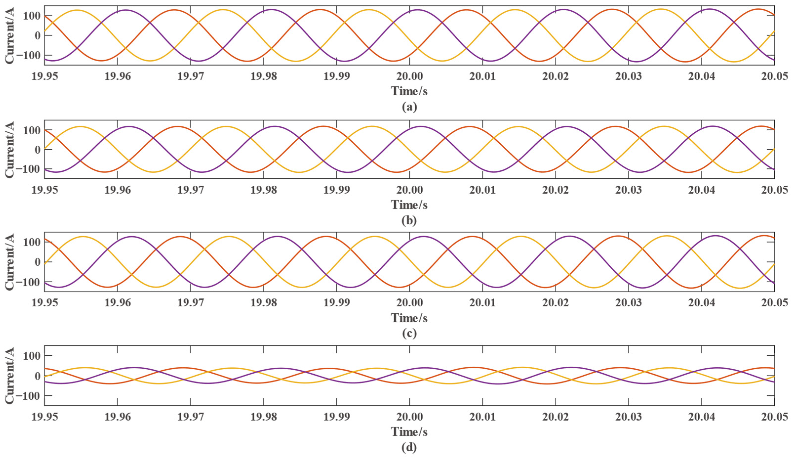
Figure 8a–d represent the currents of each component of the microgrid, and the currents of the microgrid changes continuously due to the power regulation. Figure 9 shows that although the currents of the microgrid change due to the power regulation of each component, the currents of each component are also three-phase sinusoidal waveforms in the time period from 19.95 s to 20.05 s. The orange, purple, and yellow lines in Figure 8a–d represent the output three-phase current, respectively.
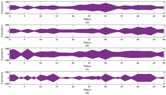
Figure 8.
Output current of each component of the microgrid: (a) output current of PV power generation; (b) output current of wind power generation; (c) output current of diesel power generation; and (d) output current of the energy storage section.
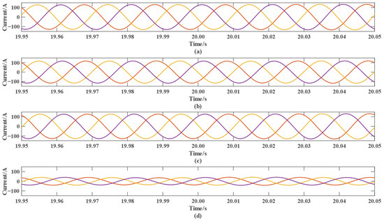
Figure 9.
Output current of the microgrid at a certain time period: (a) output current of PV power generation; (b) output current of wind power generation; (c) output current of diesel power generation; and (d) output current of the energy storage section.
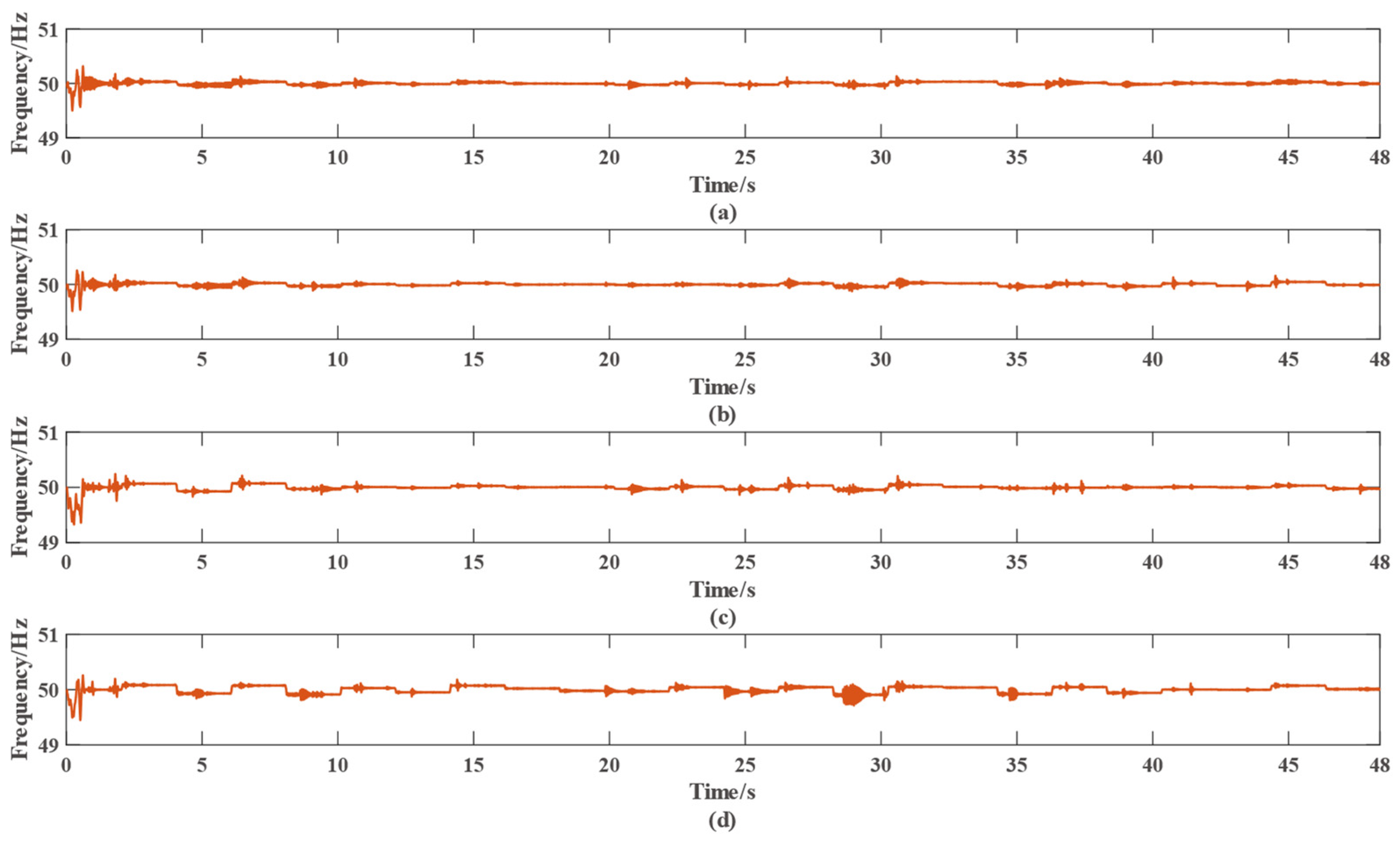
Figure 10a–d represent the frequencies of each component of the microgrid, and it can be seen that the frequencies of the output voltages fluctuate during power regulation, but they are all maintained near the desired frequency of 50 Hz, which indicates that the frequencies of the output voltages of the microgrid are stable.
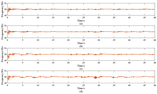
Figure 10.
Frequency of the output voltage of the microgrid: (a) frequency of the output voltage of the PV power generation; (b) frequency of the output voltage of the wind power generation; (c) frequency of the output voltage of the diesel power generation; and (d) frequency of the output voltage of the energy storage section.
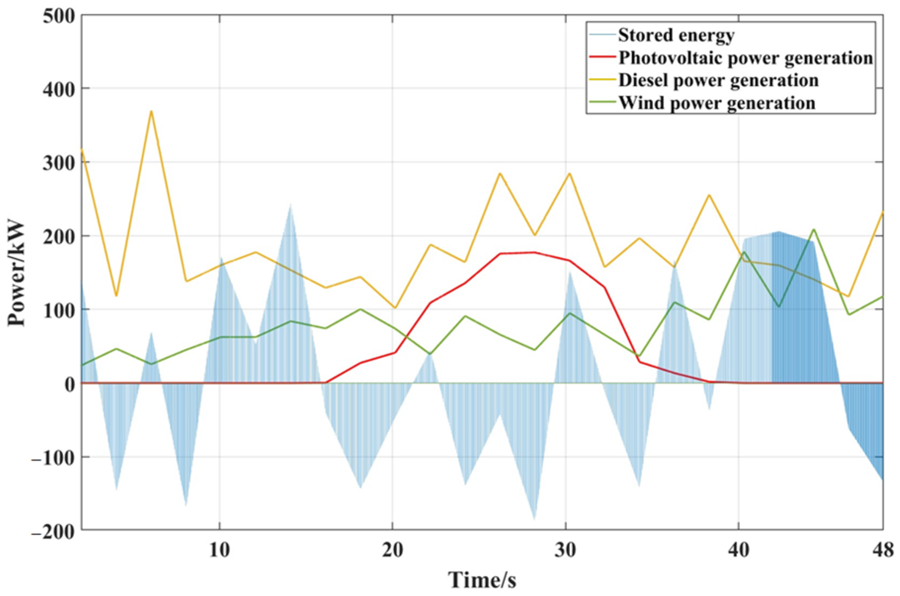
Figure 11 represents the output power of the PV, wind, diesel, and energy storage section, respectively. It can be seen by comparing this figure to Figure 5d, the output power is able to change according to the preset regulation process, which indicates that the modified particle swarm algorithm is able to carry out power scheduling in the microgrid model.
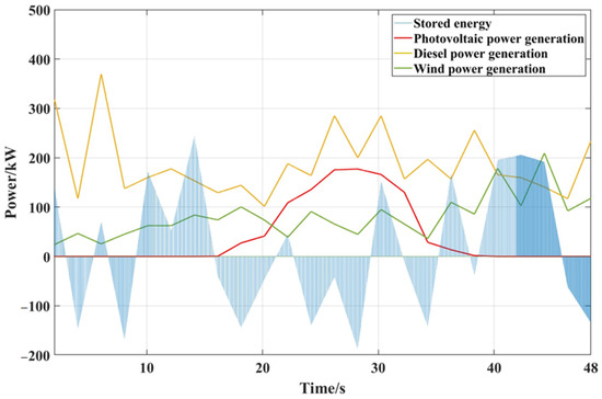
Figure 11.
Output power of each component of the microgrid.
5. Discussion of Microgrids’ Dispatch by Environmental Perturbations
5.1. Analysis of Price Changes in the New Energy Power Generation Market
During the actual operation of microgrids, microgrids’ dispatch is always affected by various factors, such as changes in power generation costs, weather changes, load changes, and so on. By simulating the real-life perturbations, observing the impact on the algorithm optimization results, and analyzing the changes in the scheduling scheme, it is helpful to provide a reference for the future development of microgrids.
According to the information released by the National Development and Reform Commission and the National Energy Administration, the cost of wind power in East China has been lowered 6 times in recent years, from RMB 0.6/kWh down to about RMB 0.5/kWh, and the cost of PV power generation has been lowered 5 times in recent years, from RMB 1.0/kWh down to about RMB 0.6/kWh. New energy prices are gradually entering the era of parity.
On this basis, the simulation of power price downward adjustment is carried out. A loop is set in the algorithm to make PV and wind prices decrease. Because the price is too low or too high to have reference significance, the upper limit of PV power price is limited to RMB 0.7/kWh, the lower limit is RMB 0.3/kWh, the modification step is 0.1, the number of times is 5; the wind power’s upper limit price is RMB 0.6/kWh, the lower limit is RMB 0.2/kWh, the modification step is 0.1, and the number of iterations is 5. The wind power absorption rate and the total surplus of power generation change as shown in Figure 12.
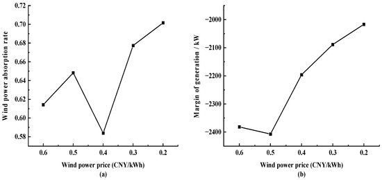
Figure 12.
Results of adjusting wind power price: (a) wind power absorption rate and (b) generation margins.
Figure 12 shows that the midway point of wind power absorption rate fluctuates, the overall trend is increasing, and the value of the total surplus of power generation is generally increasing, which indicates that the absolute value is generally decreasing, i.e., the difference between the dispatched power generation and the predicted load is shrinking. Therefore, as the price of wind power decreases, the utilization of wind turbines is increasing, and the reliability of the generation system is also increasing.
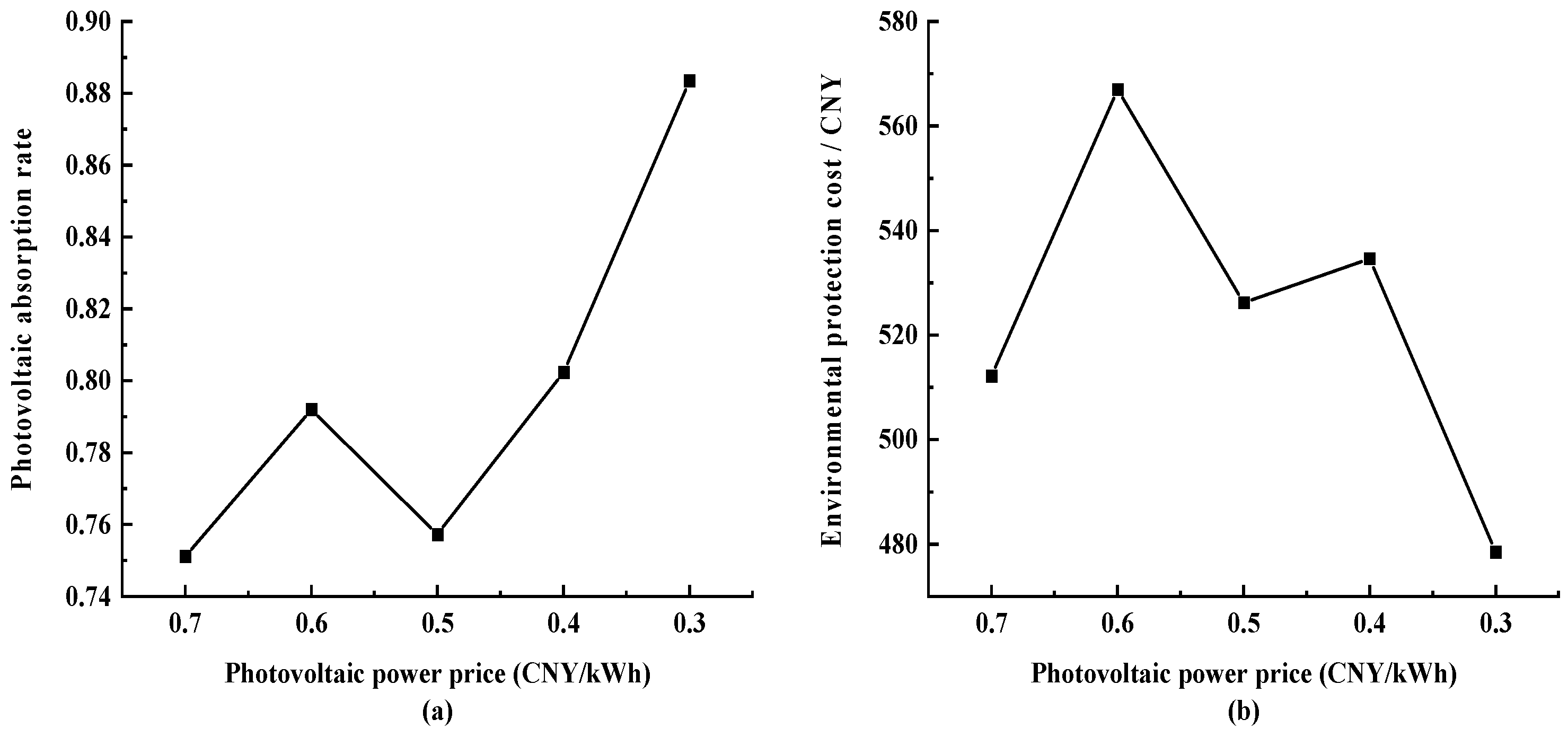
Subsequently, the fixed wind power price is RMB 0.6/kWh. Thus, the PV price must be adjusted from RMB 0.7/kWh to RMB 0.3/kWh. The results are shown in Figure 13, showing that the overall trend of the PV absorption rate is increasing, while the overall trend of the value of environmental costs is decreasing. Therefore, with the reduction in PV prices, the utilization of PV units increases, the amount of emissions that need to be handled decreases, and the environmental performance of the microgrids improves.
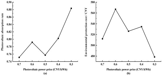
Figure 13.
Results of adjusting PV power price: (a) PV absorption rate and (b) environmental protection cost.
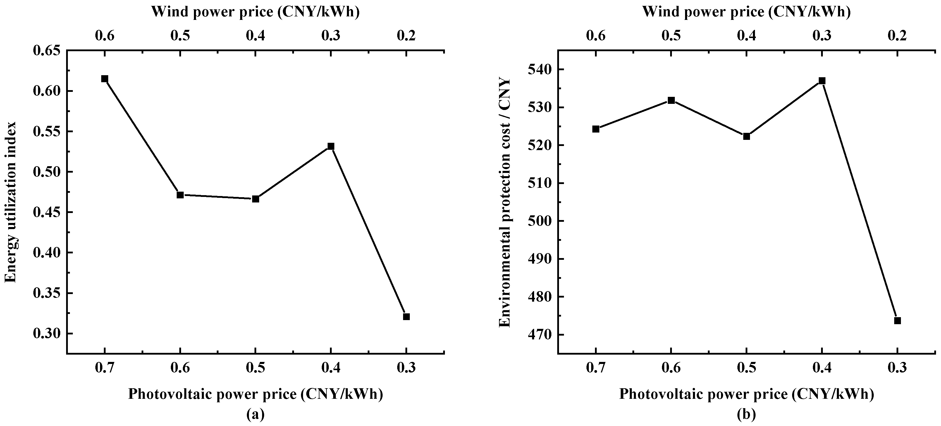
Finally, the prices of PV and wind power generation are adjusted downward at the same time, with the price of PV being adjusted downward from RMB 0.7/kWh to RMB 0.3/kWh, and the price of wind power generation is adjusted downward from RMB 0.6/kWh to RMB 0.2/kWh. The results are shown in Figure 14, showing that with the simultaneous downward adjustment of PV and wind power prices, the value of the stability index has decreased overall. With the downward adjustment of new energy prices, the utilization rate of PV and wind energy will be further improved. The experimental results show that when the price of PV is RMB 0.3/kWh and the price of wind power is RMB 0.2/kWh, the microgrid obtains the optimal environmental protection for scheduling operations.

Figure 14.
Simultaneous adjustment of PV and wind power generation price results: (a) energy utilization indicators and (b) environmental cost.
5.2. Impact of Microgrid Parameter Variations on Optimization Strategies
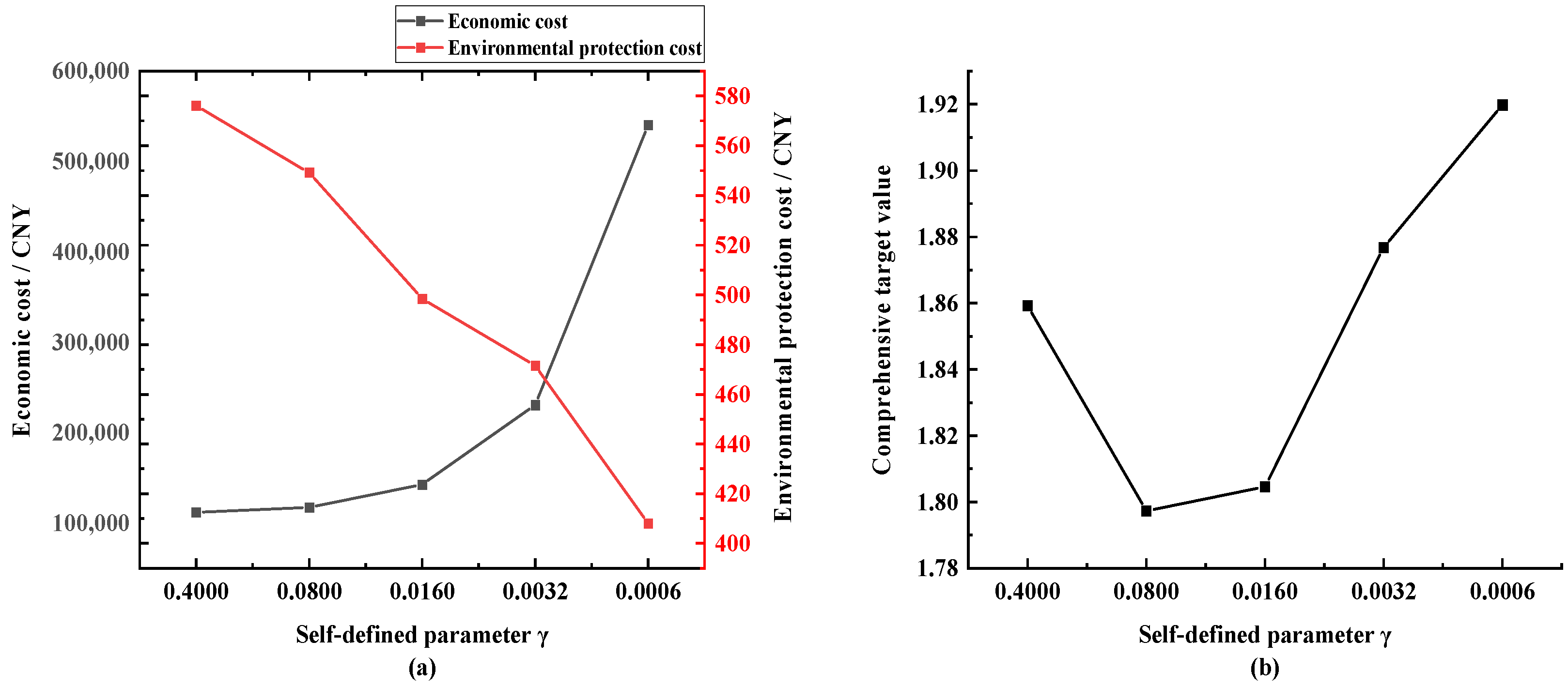
For the convenience of convergence and to quickly address particle swarm optimization, the economic and environmental indicators are combined in the objective function in Section 3.1.2 and balanced with the customized parameter γ, as detailed in Equation (15). The custom parameter γ variate affects the priority of economic and environmental costs in particle swarm optimization. In order to make a side-by-side comparison of the modified parameters’ effects, the generation capacity of the microgrid is altered to compare and analyze the relevant changes that should be made to the optimization strategy under different configurations of wind and PV power generation in the microgrid. The numerical size of the unit capacity adjustment is partially referred to in the literature [34].
The initial value of the customized parameter γ is selected as 0.4, i.e., the weight of the economic index is 0.4, and the weight of the environmental index is 0.6. Subsequently, the formula is used to reduce the value of γ sequentially, and the changes in the environmental and economic indexes are compared to the decreasing value of the weight. The results, after taking the average value of multiple runs, are shown in Figure 15.
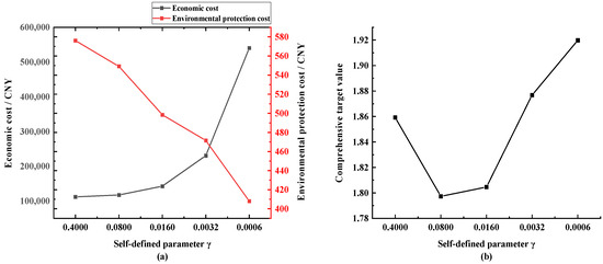
Figure 15.
Changing the economic weights γ results in (a) economic and environmental costs and (b) comprehensive target value.
Figure 15a shows that there is a conflict between the two indicators of environmental friendliness and economy, and the optimization of one indicator causes the deterioration of the other one. The main reason for this is that the improvement in environmental protection will reduce the output of the diesel engine, which may lead to an increase in the load shortage rate, and then lead to an increase in shortage costs, which will decrease the value of the economic index. Therefore, the simultaneous optimization of microgrid economy and environmental friendliness cannot be achieved; however, the corresponding compromise results can be obtained by balancing parameter γ.
The microgrid scheduling optimization of the indicators obtained in accordance with the aforementioned Section 4.1 is part of the optimal solution when the method is subjected to normalization of linear weighting to find a comprehensive value, changing the comprehensive indicator curve, as depicted in Figure 15b. The comprehensive index takes the value range of [0, 2], with a smaller value indicating that the microgrid performance is better. Thus, as the weight γ continues to decrease, the overall comprehensive microgrid performance becomes subjected to a decreasing trend, with optimal performance being achieved when γ = 0.08.
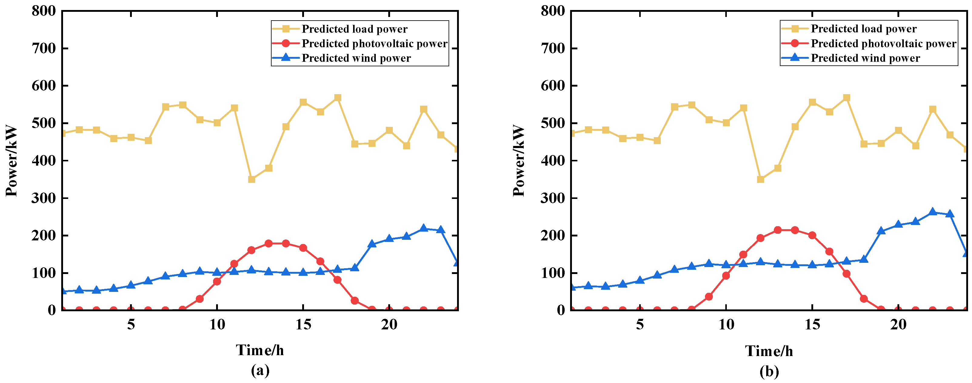
Due to the high proportion of units generating clean energy in the wind–PV–diesel–storage microgrid, the microgrid is affected by the natural environment to a correspondingly large extent. Under a similar load demand and the same constraints, the preferred generation scheduling scheme will be different if the microgrid is in a different geographical environment. In this paper, the natural environment changes are simulated by adjusting the wind and PV generation capacity of the microgrid and by making a side-by-side comparison with the results obtained from the initial microgrid data. Figure 16 depicts the adjusted and original capacity ratios when both the PV and wind power generation capacity are increased by 20%.
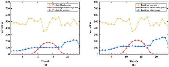
Figure 16.
Comparison of microgrid prediction curves: (a) East China power grid original configuration and (b) East China power grid configuration changes.
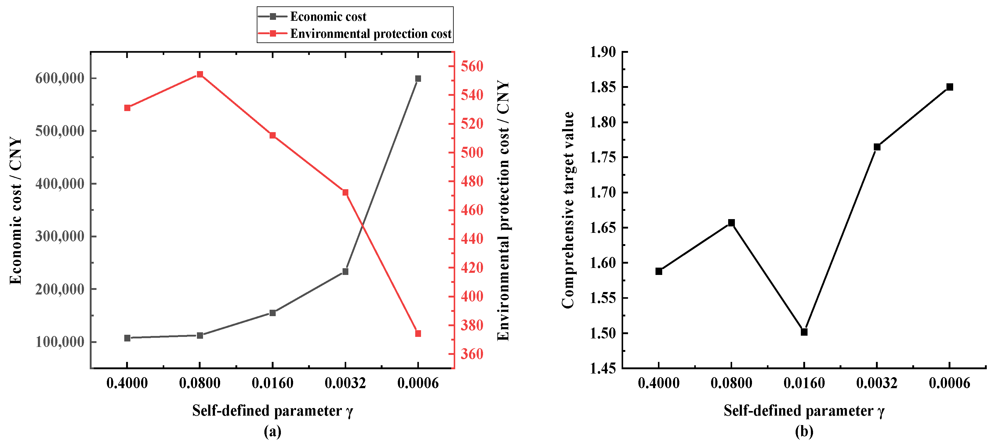
Keeping the load demand the same, a particle swarm simulation is carried out under the same constraints, the same diesel engine unit size and storage battery capacity, and with a customized parameter γ being reduced with the same tendency of variation, with the results being shown in Figure 17.

Figure 17.
Results of changing the economic weight γ after capacity configuration changes: (a) economic and environmental protection cost and (b) comprehensive target value.
As shown in Figure 17, as the customized parameter γ decreases, the economic cost gradually rises, the environmental protection cost undergoes fluctuations with an overall decreasing trend, and the economic and environmental protection indexes still show a negative correlation. The final optimal value of the multi-objective index appears in the case of custom parameter γ = 0.016, which is lower than the optimal strategy under the original configuration γ = 0.08.
The reason for this is that there is a change in capacity configuration, the new energy generation of the microgrid is improved to meet the load demand, and the original configuration is less dependent on the diesel engine to fill the gap. Therefore, appropriately increasing the cost of environmental protection and reducing the use of the diesel engine will not excessively add to the cost of power shortage, which will be burdensome to the whole grid operation. As a result of this, a better microgrid scheduling strategy is obtained. Therefore, as the surrounding environment changes, the microgrid also needs to adjust the optimization strategy in order to obtain the best operating results.
6. Conclusions
From the above simulation results, it can be understood that the modified particle swarm algorithm obtained through the introduction of variable inertia weight and learning factors has a higher utilization rate of external storage libraries and a better global convergence. Moreover, as the microgrid’s photovoltaic absorbed rate increases from 0.7724 to 0.8683 and wind energy absorbed rate from 0.6064 to 0.7158, a 14.89% increase in energy utilization and a reduction in environmental costs from RMB 135,870 to RMB 132,230 is achieved. The microgrid model built in Simulink can output stable voltage, current, and frequency, and the simulation results verify that the modified particle swarm algorithm can be applied to microgrids. As the new energy market power generation price downward adjustment of the situation as well as change in the simulation of microgrid parameters verified that there is a conflict between the economic and environmental protection indexes by adjusting the microgrids’ wind power generation component capacity for a comparison test, we studied the impact of different capacity configurations on the optimization results of microgrid scheduling. Furthermore, we verified the need to reasonably determine the value of custom parameter γ according to the actual situation of the microgrid in order to adjust the optimization strategy. However, the particle swarm algorithm still has the possibility of falling into a local optimal solution. In the future, the researchers would like to adopt a multiple restart strategy, using different random seeds, initial positions, and speeds each time. The instability of the algorithm due to different initial states can be mitigated by comparing the results of multiple independent runs. This could be performed by introducing more intelligent and flexible neighborhood search mechanisms, such as introducing changing neighborhood sizes or neighborhood shapes, as well as introducing an adaptive mechanism that allows the algorithm to automatically adjust the algorithm parameters according to the current search state.
Author Contributions
Y.S. introduced the principle of hierarchical control of an AC microgrid; K.F. carried out the particle swarm algorithm’s simulation; X.W. added the optimization results of the particle swarm algorithm to the Simulink model of the microgrid, carried out the simulation, plotted the graphs of ++each parameter of the microgrid’s outputs, analyzed the data, and wrote this article under the guidance of Y.S. All authors have read and agreed to the published version of the manuscript.
Funding
This work was supported by the National Natural Science Foundation of China (62303107), the Shanghai Sailing Program (21YF1400100), and the Fundamental Research Funds for the Central Universities (2232021D-38, 2232022G-09).
Institutional Review Board Statement
Not applicable.
Informed Consent Statement
Not applicable.
Data Availability Statement
Data are contained within the article.
Conflicts of Interest
The authors declare no conflicts of interest.
References
- Huang, S.; Wu, Q.; Liao, W.; Wu, G.; Li, X.; Wei, J. Adaptive Droop-Based Hierarchical Optimal Voltage Control Scheme for VSC-HVdc Connected Offshore Wind Farm. IEEE Trans. Ind. Inform. 2021, 17, 8165–8176. [Google Scholar] [CrossRef]
- Liang, Z.; Dong, Z.; Li, C.; Wu, C.; Chen, H. A Data-Driven Convex Model for Hybrid Microgrid Operation with Bidirectional Converters. IEEE Trans. Smart Grid 2023, 14, 1313–1316. [Google Scholar] [CrossRef]
- Shan, Y.; Ma, L.; Yu, X. Hierarchical Control and Economic Optimization of Microgrids Considering the Randomness of Power Generation and Load Demand. Energies 2023, 16, 5503. [Google Scholar] [CrossRef]
- Che, L.; Shahidehpour, M.; Alabdulwahab, A.; Al-Turki, Y. Hierarchical Coordination of a Community Microgrid with AC and DC Microgrids. IEEE Trans. Smart Grid 2015, 6, 3042–3051. [Google Scholar] [CrossRef]
- Mutarraf, M.U.; Guan, Y.; Terriche, Y.; Su, C.; Nasir, M.C.; Vasquez, J.M.; Juerrero, J. Adaptive Power Management of Hierarchical Controlled Hybrid Shipboard Microgrids. IEEE Access 2022, 10, 21397–21411. [Google Scholar] [CrossRef]
- Xin, H.; Zhao, R.; Zhang, L.; Wang, Z.; Wong, K.P.; Wei, W. A Decentralized Hierarchical Control Structure and Self-Optimizing Control Strategy for F-P Type DGs in Islanded Microgrids. IEEE Trans. Smart Grid 2016, 7, 3–5. [Google Scholar] [CrossRef]
- Wu, X.; Xu, Y.; He, J.; Wang, X.; Vasquez, J.C.; Guerrero, J.M. Pinning-Based Hierarchical and Distributed Cooperative Control for AC Microgrid Clusters. IEEE Trans. Power Electron. 2020, 35, 9865–9885. [Google Scholar] [CrossRef]
- Tian, P.; Xiao, X.; Wang, K.; Ding, R. A Hierarchical Energy Management System Based on Hierarchical Optimization for Microgrid Community Economic Operation. IEEE Trans. Smart Grid 2016, 7, 2230–2241. [Google Scholar] [CrossRef]
- Hong, Y.; Alano, F.I. Hierarchical Energy Management in Islanded Networked Microgrids. IEEE Access 2022, 10, 8121–8132. [Google Scholar] [CrossRef]
- Agundis-Tinajero, G.; Aldana, N.L.D.; Luna, A.C.; Segundo-Ramírez, J.; Visairo-Cruz, N.; Guerrero, J.M.; Vazquez, J.C. Extended-Optimal-Power-Flow-Based Hierarchical Control for Islanded AC Microgrids. IEEE Trans. Power Electron. 2019, 34, 840–848. [Google Scholar] [CrossRef]
- Baghaee, H.R.; Mirsalim, M.; Gharehpetian, G.B. Performance Improvement of Multi-DER Microgrid for Small- and Large-Signal Disturbances and Nonlinear Loads: Novel Complementary Control Loop and Fuzzy Controller in a Hierarchical Droop-Based Control Scheme. IEEE Syst. J. 2018, 12, 444–451. [Google Scholar] [CrossRef]
- Wang, H.; Xing, H.; Luo, Y.; Zhang, W. Optimal scheduling of micro-energy grid with integrated demand response based on chance-constrained programming. Int. J. Electr. Power Energy Syst. 2023, 144, 108602. [Google Scholar] [CrossRef]
- Pournazarian, B.; Sangrody, R.; Saeedian, M.; Lehtonen, M.; Pouresmaeil, E. Simultaneous Optimization of Virtual Synchronous Generators (VSG) Parameters in Islanded Microgrids Supplying Induction Motors. IEEE Access 2021, 9, 124972–124985. [Google Scholar] [CrossRef]
- Borghei, M.; Ghassemi, M. A Multi-Objective Optimization Scheme for Resilient, Cost-Effective Planning of Microgrids. IEEE Access 2020, 8, 206325–206341. [Google Scholar] [CrossRef]
- Fan, Z.; Wan, Z.; Gao, L.; Xiong, Y.; Song, G. A Multi-Objective Optimal Configuration Method for Microgrids Considering Zero-Carbon Operation. IEEE Access 2023, 11, 87366–87379. [Google Scholar] [CrossRef]
- Tan, B.; Chen, H. Stochastic Multi-Objective Optimized Dispatch of Combined Cooling, Heating, and Power Microgrids Based on Hybrid Evolutionary Optimization Algorithm. IEEE Access 2019, 7, 176218–176232. [Google Scholar] [CrossRef]
- Zhang, Z.; Wang, Z.; Wang, H.; Zhang, H.; Yang, W.; Cao, R. Research on Bi-Level Optimized Operation Strategy of Microgrid Cluster Based on IABC Algorithm. IEEE Access 2021, 9, 15520–15529. [Google Scholar] [CrossRef]
- Yuan, W.; Wang, Y.; Chen, Z. New Perspectives on Power Control of AC Microgrid Considering Operation Cost and Efficiency. IEEE Trans. Power Syst. 2021, 36, 4844–4847. [Google Scholar] [CrossRef]
- Zhu, X.; Peng, C.; Geng, H. Multi-Objective Sizing Optimization Method of Microgrid Considering Cost and Carbon Emissions. In Proceedings of the 2022 4th International Conference on Smart Power & Internet Energy Systems (SPIES), Beijing, China, 9–12 December 2022. [Google Scholar] [CrossRef]
- Zhu, Z.; Zhang, Z.; Man, W.; Tong, X.; Qiu, J.; Li, F. A new beetle antennae search algorithm for multi-objective energy management in microgrid. In Proceedings of the 2018 13th IEEE Conference on Industrial Electronics and Applications (ICIEA), Wuhan, China, 31 May–2 June 2018. [Google Scholar] [CrossRef]
- Alkebsi, K.; Du, W. A Fast Multi-Objective Particle Swarm Optimization Algorithm Based on a New Archive Updating Mechanism. IEEE Access 2020, 8, 124734–124754. [Google Scholar] [CrossRef]
- Khalil, A.; Boghdady, T.A.; Alham, M.H.; Ibrahim, D.K. Enhancing the Conventional Controllers for Load Frequency Control of Isolated Microgrids Using Proposed Multi-Objective Formulation via Artificial Rabbits Optimization Algorithm. IEEE Access 2023, 11, 3472–3493. [Google Scholar] [CrossRef]
- Alvarez, J.A.M.; Zurbriggen, I.G.; Paz, F.; Ordonez, M. Microgrids Multiobjective Design Optimization for Critical Loads. IEEE Trans. Smart Grid 2023, 14, 17–28. [Google Scholar] [CrossRef]
- Fang, S.; Xu, Y.; Li, Z.; Zhao, T.; Wang, H. Two-Step Multi-Objective Management of Hybrid Energy Storage System in All-Electric Ship Microgrids. IEEE Trans. Veh. Technol. 2019, 68, 3361–3373. [Google Scholar] [CrossRef]
- Zeng, Y.; Zhao, H.; Liu, C.; Chen, S.; Hao, X.; Sun, X.; Zhang, J. Multi objective optimization of microgrid based on Improved Multi-objective Particle Swarm Optimization. In Proceedings of the 2022 International Seminar on Computer Science and Engineering Technology (SCSET), Indianapolis, IN, USA, 8–9 January 2022. [Google Scholar] [CrossRef]
- Naderi, E.; Mirzaei, L.; Trimble, J.P.; Cantrell, D.A. Multi-Objective Optimal Power Flow Incorporating Flexible Alternating Current Transmission Systems: Application of a Wavelet-Oriented Evolutionary Algorithm. Electr. Power Compon. Syst 2023, 1–30. [Google Scholar] [CrossRef]
- Naderi, E.; Mirzaei, L.; Pourakbari-Kasmaei, M.; Cerna, F.V.; Lehtonen, M. Optimization of active power dispatch considering unified power flow controller: Application of evolutionary algorithms in a fuzzy framework. Evol. Intell 2023. [Google Scholar] [CrossRef]
- Li, P.; Xu, D.; Zhou, Z.; Lee, W.; Zhao, B. Stochastic Optimal Operation of Microgrid Based on Chaotic Binary Particle Swarm Optimization. IEEE Trans. Smart Grid 2016, 7, 66–73. [Google Scholar] [CrossRef]
- Yang, H.; Cai, D.; Bamisile, O.; Li, J.; Zhang, Z.; Huang, Q. Optimization of Low-carbon Dispatching for Microgrid Based on Improved Particle Swarm Optimization. In Proceedings of the 2022 IEEE 6th Conference on Energy Internet and Energy System Integration (EI2), Chengdu, China, 11–13 November 2022. [Google Scholar] [CrossRef]
- Hu, Z. Research on Multi-Objective Optimal Scheduling of Microgrid Based on Improved Particle Swarm Optimization Algorithm. Master’s Thesis, Nanchang University, Nanchang, China, 7 June 2021. [Google Scholar]
- Zeng, P. Research on Distributed Power access Optimization of Microgrid Based on Improved Particle Swarm Optimization. Master’s Thesis, Shanghai Jiao Tong University, Shanghai, China, 1 January 2015. [Google Scholar]
- Liao, Z. Research on Optimal Operation of Microgrid Based on Improved Particle Swarm Optimization Algorithm. Master’s Thesis, Nanchang University, Nanchang, China, 25 May 2019. [Google Scholar]
- Hu, L.; Liu, T.; Hou, M. Capacity optimization allocation of wind/photovoltaic/diesel/storage based on immune particle swarm optimization. Sci. Technol. Eng. 2020, 20, 14967–14973. [Google Scholar]
- Javidsharifi, M.; Arabani, H.P.; Kerekes, T.; Sera, D.; Guerrero, J.M. Quantifying the Impact of Different Parameters on Optimal Operation of Multi-Microgrid Systems. In Proceedings of the 2022 IEEE 7th Forum on Research and Technologies for Society and Industry Innovation (RTSI), Paris, France, 24–26 August 2022. [Google Scholar] [CrossRef]


Disclaimer/Publisher’s Note: The statements, opinions and data contained in all publications are solely those of the individual author(s) and contributor(s) and not of MDPI and/or the editor(s). MDPI and/or the editor(s) disclaim responsibility for any injury to people or property resulting from any ideas, methods, instructions or products referred to in the content. |
© 2024 by the authors. Licensee MDPI, Basel, Switzerland. This article is an open access article distributed under the terms and conditions of the Creative Commons Attribution (CC BY) license (https://creativecommons.org/licenses/by/4.0/).