Abstract
The paper contributes to the Sustainable Development Goals (SDGs) targeting Life Below Water by introducing user-friendly modeling approaches. It delves into the impact of abiotic factors on the first two trophic levels within the marine ecosystem, both naturally and due to human influence. Specifically, the study examines the connections between environmental parameters (e.g., temperature, salinity, nutrients) and plankton along the Romanian Black Sea coast during the warm season over a decade. The research develops models to forecast zooplankton proliferation using machine learning (ML) algorithms and gathered data. Water temperature significantly affects copepods and “other groups” of zooplankton densities during the warm season. Conversely, no discernible impact is observed on dinoflagellate Noctiluca scintillans blooms. Salinity fluctuations notably influence typical phytoplankton proliferation, with phosphate concentrations primarily driving widespread blooms. The study explores two scenarios for forecasting zooplankton growth: Business as Usual, predicting modest increases in temperature, salinity, and constant nutrient levels, and the Mild scenario, projecting substantial temperature and salinity increases alongside significant nutrient decrease by 2042. The findings underscore high densities of Noctiluca scintillans under both scenarios, particularly pronounced in the second scenario, surpassing the first by around 70%. These findings, indicative of a eutrophic ecosystem, underscore the potential implications of altered abiotic factors on ecosystem health, aligning with SDGs focused on Life Below Water.
1. Introduction
The oceans play a crucial role in providing essential services to both humanity and the planet [1,2,3]. However, the deterioration of its health, productivity, and resilience, primarily caused by escalating human pressures, including land-based pollution, the warming and sea-level rise induced by climate change, ocean acidification, and over-exploitation of marine resources, poses a significant threat [4,5,6,7]. This decline jeopardizes the achievement of adequate nutrition, sustainable livelihoods, and economic growth, particularly for coastal communities. Additionally, it adversely impacts other vital ecosystem services, such as recreation and coastal protection. Global endeavors for Sustainable Development Goal 14 (SDG 14)—Life Below Water—are primarily centered on confronting challenges and enhancing the well-being of the world’s oceans, seas, and marine ecosystems [8,9]. The achievement of SDG 14 relies heavily on advancements made in other interconnected goals [10]. With its extensive presence on Earth, Life Below Water serves as a pivotal nexus, intricately linking and influencing various Sustainable Development Goals (SDGs) [11]. Its impact extends beyond marine health, due to its economic impact resonating with SDG 1 (No Poverty), by supporting coastal communities dependent on marine resources through healthy oceans and seas, and SDG 2 (Zero Hunger) through sustainable fisheries and aquaculture practices, which supports food security [12]. Moreover, it aligns with SDG 3 (Good Health and Well-being) by preserving biodiversity and providing resources for medicine, SDG 6 (Clean Water and Sanitation) through pollution prevention and ensuring sustainable water resources, and SDG 13 (Climate Action) by mitigating climate change effects, in which oceans play a crucial role by absorbing carbon dioxide and heat [13]. This intricate interplay underscores the indispensable role of Life Below Water in shaping a sustainable and interconnected future. Expanding its connections to other SDGs, Life Below Water promotes environmental education and fostering community awareness, addressing SDG 4 (Quality Education). It recognizes the vital roles of women in coastal communities, contributing to SDG 5 (Gender Equality), and explores sustainable energy solutions like wave and tidal energy, aligning with SDG 7 (Affordable and Clean Energy). Additionally, it fosters sustainable livelihoods, economic growth, and decent work opportunities, aligning with SDG 8 (Decent Work and Economic Growth) [14], and encourages innovations in sustainable marine practices, in line with SDG 9 (Industry, Innovation, and Infrastructure), for fisheries, tourism, and shipping industries. The health and well-being of marine ecosystems play a pivotal role in addressing social inequalities, aligning with SDG 10 (Reduced Inequality) by ensuring equitable access to marine resources and benefits. Sustainable coastal development and resilient communities harmonizing with marine ecosystems correspond to SDG 11 (Sustainable Cities and Communities), while responsible consumption and production practices are integral to SDG 12 (Responsible Consumption and Production). Recognizing the interconnectedness of marine and terrestrial ecosystems responds to SDG 15 (Life on Land)—conservation efforts in one area have positive effects on the other, promoting biodiversity and ecosystem resilience. In the context of ongoing global challenges, governance structures ensuring sustainable management and conservation of marine resources resonate with SDG 16 (Peace, Justice, and Strong Institutions), while collaborative partnerships addressing the complex challenges facing Life Below Water align with SDG 17 (Partnerships for the Goals) [15,16].
In essence, achieving Life Below Water standards and SDG 14 is imperative for a sustainable society. SDG 14 acts as a catalyst for a sustainable and interconnected future, embodying the spirit of the 2030 Agenda and emphasizing the necessity for collaborative efforts across all dimensions of sustainable development [17,18,19].
Marine plankton species diversity governs one of the most essential ecosystem functions—biological productivity [20]. Phytoplankton are responsible for the annual production of approximately 50% of the Earth’s net primary production [21]. They are mainly consumed by zooplankton, which in turn supports planktivorous fish production. Together with the ecosystem’s structure, which contains its biotic and abiotic elements, these functions generate an essential service—the habitat [22]—which, if healthy, creates significant social and economic benefits for the coastal community. Romania’s “Blue Economy” sector is undeveloped compared with other European Union (EU) member states and with other national economic sectors. With just over EUR one billion, it represented, in 2018, 0.6% of the national economy and 66,600 jobs [23]. The living resources sector generated only EUR 85 million and 6200 jobs. Excluding issues related to legislative gaps and organizational shortcomings (such as the absence of a maritime spatial plan and the failure to designate areas for aquaculture), it can be said that the growth prospects rely on the well-being of the ecosystem. The ecosystem’s health depends mainly on the intensity of the pressures it is subjected to. The northwestern area of the Black Sea has endured, over time, several abrupt changes in the transition from a low-production system (the 1970s) to a highly eutrophicated system (the 1980s) and then an intermediate state with relatively low biomass (1990s–2000s), when bacterioplankton, zooplankton, and living marine resources had low quantities. Still, the nonfodder component of zooplankton (Noctiluca scintillans) and gelatinous organisms were at moderate levels, indicating a degraded ecosystem [24] and not a trend of improvement and rehabilitation [25]. All these regimes were mainly driven by nutrient discharges from point and diffuse sources. Nowadays, to these are added the effects of climate change, i.e., warming of the seawater, which is expected to cause the extinction of some species in the future by exceeding their thermal limit as well as restructuring of the community’s composition, both associated with possible consequences on the functioning of the marine food chain and biogeochemical cycles [20].
Unfortunately, current managerial practices are ineffective in managing complex phenomena, such as ecosystem regime changes, due to the lack of adequate explanatory models [26]. Thus, using semi-quantitative modeling (Fuzzy Cognitive maps—FCMs) coupled with statistical methods (Machine Learning—ML) to assess the natural and anthropogenic variability of the relationships between abiotic factors and different trophic levels of the marine ecosystem can facilitate the understanding of less-known processes that may occur within the ecosystem [27,28].
The study achieved this by applying semi-quantitative modeling (FCMs) and machine learning (ML) algorithms to create the model for generating applicable predictions in decision making regarding managing pressures on the marine ecosystem. Thus, for the success of decisions, the model can distinguish between factors by generating robust results and improving case study analysis methods [29].
However, implementing ML techniques is not always straightforward and presents several challenges and potential pitfalls. Conversely, these methods present many opportunities and can yield fresh and valuable insights [30]. Thus, secondly, Machine Learning techniques like Forest-based Classification and Regression improved FCMs’ predictive capabilities by learning from data patterns and adapting to new information, making the model more accurate [31]. When properly trained, these models can predict changes in temperature, salinity, nutrient levels, and the population of plankton species, aiding in forecasting ecosystem changes [32]. We thoroughly searched through available resources but did not uncover any papers detailing the integration of Fuzzy Cognitive Maps (FCMs) with machine learning (ML) techniques like Forest-based Classification and Regression.
Consequently, this work contributes significantly to the Sustainable Development Goals (SDGs) related to Life Below Water by offering accessible modeling methods [27,28,33]. It focuses on understanding how abiotic factors impact the initial two levels of the marine ecosystem through natural processes and human influence. The study develops predictive models using the identification of the main drivers by FCMs and machine learning (ML) algorithms based on collected data, to forecast the proliferation of zooplankton. Utilizing machine learning (ML) algorithms to forecast zooplankton proliferation offers a data-driven method to predict ecosystem behavior, providing a more nuanced understanding than traditional modeling approaches. ML excels at handling complex, nonlinear relationships within data, potentially capturing intricate patterns that conventional statistical methods might miss [34]. Consequently, combining fuzzy cognitive maps with machine learning techniques can provide valuable insights into complex ecological systems. However, it is crucial to cautiously approach their development and implementation, ensuring robust data, validation procedures, and a clear understanding of the system’s dynamics and limitations [35].
The study aims to introduce qualitative and semi-quantitative modeling along with machine learning algorithms. The primary focus is running scenarios using these methodologies to predict the ecosystem’s behavior. Additionally, the objective is to assess the natural variability and anthropogenic impact of the relationships between abiotic factors and the first two trophic levels of the marine ecosystem.
2. Materials and Methods
Seawater and biological (for phytoplankton and zooplankton) samples were collected in expeditions organized in the warm season (from May to September) of 2008–2018 in the Black Sea monitoring network, consisting of 39 stations located in variable-salinity, coastal, and marine waters (Figure 1). The year 2012 was not included in the analysis, as expeditions were undertaken only in the cold season this year. Modeling the biotic component of the ecosystem requires long-term data characterizing the entire habitat. Therefore, we used physical and chemical parameters that intervene in plankton development, collected simultaneously (temperature, salinity, and nutrients). On the other hand, this very comprehensive data set helps eliminate the difference in time between the occurrence of changes in abiotic and biotic components. After 2018, the sampling frequency decreased due to the COVID-19 pandemic and, recently, due to the war in Ukraine.
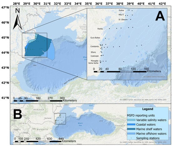
Figure 1.
Map of the study area. The square shows the location of the sampling sites on the Romanian coastline (A) and the position in the Black Sea region (B).
Phytoplankton (N = 7956) and zooplankton (N = 7956) samples were collected and analyzed according to previously described methodology [36,37].
Temperature and salinity (N = 7950) were measured using the reversible thermometer, the titration method, and the CastAway CTD multiparameter probe (YSI Cast Away model).
Dissolved nutrient concentrations (phosphates and silicates, N = 7950; nitrites, nitrates, and ammonia, N = 7861) were determined according to standard methods for seawater analysis [38].
Data statistics and their visualization were performed with STATISTICA 14.0.0.15 [39], an advanced software package that provides data analysis, data management, statistics, data mining, machine learning, text analysis, and data visualization procedures. The data were analyzed by general descriptive statistics and visualized (boxplot); then, the correlations between the parameters (Pearson coefficient, r) were performed, which determined the extent to which the values of the two variables were “proportional” to each other. The significance level (p) calculated for each correlation is a primary source of information about the reliability of the correlation. In the statistical analysis, the threshold value p = 0.05 and enough data (more than 7500 for each variable) were used to respect the hypothesis of normality.
The semi-quantitative modeling was carried out with the Mental Modeler software, a decision support software (open-source, https://www.mentalmodeler.com/) that helps experts understand the impact associated with environmental changes and develop strategies for reducing unwanted outcomes by capturing, communicating, and representing knowledge. By building Cognitive Knowledge Maps (FCMs), the Mental Modeler allows the development of a semi-quantitative model that (1) defines the important components, (2) defines the strength of the relationships between the components, and (3) runs scenarios that determine how the system reacts in certain conditions [40].
ArcGIS Desktop 10.7 software (ESRI, 2019) [41] was used to create distribution maps and machine learning (ML) algorithms. The basic premise of ML is that a machine (e.g., an algorithm or model) can make predictions based on existing data. The basic technique behind all ML methods is an iterative combination of statistics and error minimization, applied and combined to varying degrees. Many ML algorithms iteratively check all or many possible outcomes to find the best outcome for the problem. The potentially large number of iterations is prohibitive for manual calculations and is a large part of why these methods are only now widely available to individual researchers.
- The first step in applying ML was to learn the algorithm using the training dataset (2008–2018), which consists of the independent variables (abiotic components—T, S, PO4, DIN) with dependent variables (total phytoplankton density). The training data is used to “learn” how the independent (input) variables relate to the dependent (output) variable.
- In step two, when the algorithm is applied to new input data, corresponding to the scenarios to be tested, the model applies the learned relationship and returns a prediction. After the algorithm is trained, it must be tested to measure the quality of predictions from new data.
- This requires another data set with independent and dependent variables, but the dependent (target) variables (10–20% of the original data) are not provided. Algorithm predictions (output) are compared with retained data (target) to validate the algorithm. This comparison represents the significant difference between ML and traditional statistical techniques that use p-values for validation [40].
ArcGIS creates models and generates predictions using an adaptation of the random forest algorithm (Leo Breiman) called Forest-based Classification and Regression [42], a supervised machine learning method. Predictions can be made for categorical (classification) and continuous (regression) variables. By default, ML uses 90% of the data to build the model and 10% to validate it (Figure 2).

Figure 2.
Flowchart of the methodology for modeling dynamic processes in the Black Sea pelagic habitat—causal connections between abiotic and biotic factors in two climate change scenarios.
Two scenarios for forecasting the growth of zooplankton were developed and analyzed: Business as Usual, in which temperature increases by 0.4 °C, salinity increases by 0.84‰, and nutrient levels remain constant, and the Mild scenario, in which sea water temperature increases by 0.8 °C, salinity increases by 1.68‰, and nutrients concentrations are decreased by 25% for phosphates and 70% for inorganic nitrogen until 2042.
3. Results
This section is subdivided into three key components, each focusing on distinct aspects of ecosystem analysis. The first, Section 3.1, explores the construction of a semi-quantitative model, delineating the interdependent relationships between environmental factors and specific trophic levels within the ecosystem. The second (Section 3.2) delves into the exploration of potential ecosystem evolution scenarios, employing Fuzzy Cognitive Maps (FCMs) and Machine Learning (ML) methodologies, particularly under the influence of climate change along the Romanian Black Sea coast. The last one (Section 3.3) outlines anticipated directions for future research, focusing on hypotheses regarding planktonic proliferations in the Romanian Black Sea area, intending to expand and deepen the understanding of ecosystem dynamics and responses to environmental changes.
3.1. Semi-Quantitative Model of Causal Relationships between Abiotic Factors (Temperature, Salinity, and Nutrients) and Two Trophic Levels
The water temperature ranged from 13.5 °C to 28.0 °C, and the variability expressed as standard deviation was 3.51 °C. An increasing trend was observed over the entire analyzed period, of 0.18 °C, equivalent to an average of 0.02 °C/year. The salinity ranged from 0.11 to 20.00‰, with values lower than 6.06‰ being uncharacteristic (outliers). During the warm season, salinity variations showed a noticeable upward trend, with an increase of 0.42‰ (Table S1 and Figure 3). This variation is primarily attributed to the significant influence of evaporation and the mixing of water masses, which surpasses the impact of river and precipitation input.
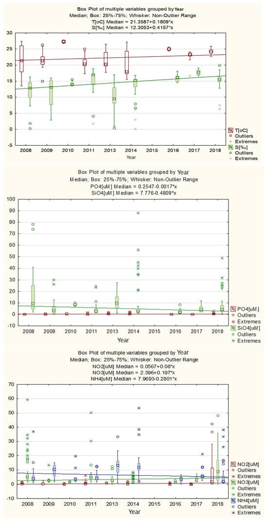
Figure 3.
Annual variation of temperature, salinity, and nutrients—Romanian Black Sea coast, 2008–2018, warm season.
Against the backdrop of increasingly dry summers, a slight decrease in phosphates and silicates was also observed, nutrients whose external input is influenced mainly by river input and continental drainage (Figure 3) (rpo4-s = −0.37; rsio4-s = −0.72). The levels of inorganic nitrogen forms (nitrites, nitrates, ammonium) have different variations during the period analyzed. Thus, nitrites and nitrates have increasing trends, by 0.08 µM and 0.20 µM, respectively, while ammonium decreases by 0.28 µM (Figure 3).
In all cases, uncharacteristic values (outliers) and extremes of the concentrations of nutrients dissolved in seawater were also observed.
Within the phytoplankton assembly, a total of 298 species were distinguished, spanning diverse varieties and forms spread across 16 taxonomic classes (Bacillariophyceae, Chlorodendrophyceae, Chlorophyceae, Chrysophyceae, Conjugatophyceae, Cryptophyceae, Cyanophyceae, Dictyochophyceae, Dinophyceae, Ebriophyceae, Euglenoidea, Prasinophyceae, Prymnesiophyceae, Trebouxiophyceae, Ulvophyceae, and Xanthophyceae). The peak species count, 160, occurred in 2013, while the lowest count, 71, was recorded in 2016. Diatoms (102 species) and dinoflagellates (76 species) constituted the majority, contributing to 60% of the overall species diversity, followed by chlorophytes (46 species) and cyanobacteria (31 species) at 15% and 10%, respectively. In less diverse classes (comprising 5 to 14 species), the Trebouxiophyceae class contributed 5% to the total species count, while Euglenoidea and Cryptophyceae represented 2% each. Classes exhibiting lower diversity (containing one to four species), including Chlorodendrophyceae, Conjugatophyceae, Chrysophyceae, Dictyochophyceae, Ebriophyceae, Prymnesiophyceae, Ulvophyceae, and Xanthophyceae, collectively constituted 6% of the qualitative composition (Figure 4). The yearly means for overall phytoplankton density fluctuated between 245.33 × 10³ cells/L (2016) and 4.10 × 10⁶ cells/L (2014). Regarding biomass, the average annual values ranged from 370 mg/m3 (in 2016) to 2820 mg/m3 (2009) (Table S1).

Figure 4.
Phytoplankton composition from the Romanian Black Sea coast, 2008–2018, warm season.
Between 2008 and 2018, 32 zooplankton taxa were identified, with the highest count found in waters with variable salinity under the Danube’s discharge influence. Copepods prevailed across all marine regions, followed by ten species of cladocerans in areas with variable salinity. The meroplanktonic group encompassed six taxa, while the “other groups” category included three species (Figure 5). Along the entire Black Sea coast, the nonfodder component was evident, with the dinoflagellate N. scintillans being the sole representative species (Figure 6). Fodder zooplankton exhibited fluctuations in density and biomass, reaching a peak annual density of 51,430 ind/m3 and a maximum annual biomass of 1539 mg/m3 in 2018 (Table S1).
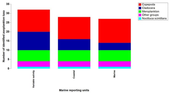
Figure 5.
Zooplankton composition from the Romanian Black Sea coast, 2008–2018, warm season.
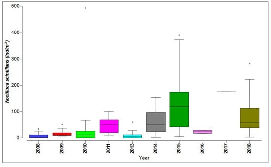
Figure 6.
Distribution of Noctiluca scintillans from the Romanian Black Sea coast, 2008–2018, warm season.
N. scintillans exhibited notable quantitative fluctuations, particularly high biomass and density, observed in 2010, 2015, and 2018, marked by some atypical values (outliers) (Figure 5).
The analysis of significant correlations between the three levels of the marine ecosystem (abiotic components—temperature, salinity, and nutrients; phytoplankton—species densities; and zooplankton—group densities) led to the creation of the Mental Modeler model. Examining the noteworthy correlations among the abiotic and biotic components resulted in the development of the Mental Modeler model.
In this context, the “models” aim is not to predict the state of this intricate ecosystem but rather to semi-quantitatively assess (using significant correlation coefficients) the connections among the various components. These connections serve as working hypotheses in the subsequent development of scenarios. Thus, FCM uses three characteristics of the studied system:
- −
- System components (N = 89)—abiotic parameters (T, S, nutrients), phytoplankton species with more than ten occurrences, zooplankton groups;
- −
- Positive or negative relationships between components (N = 203)—significant correlations, greater than ±0.50, between components;
- −
- The degree of influence that one component can have on another, defined by qualitative weights—as the significant correlations (p < 0.05) coefficient between the system components (Table S2).
Thus, apart from temperature as the main abiotic driver, the model identified as the main “drivers” (out of a total of 31), in order of importance, the concentrations of silicates and ammonium, and as “receivers” (out of a total of 26) the densities of “other groups” and copepods (Figure 7).
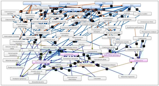
Figure 7.
Fuzzy Cognitive Map (FCM)—the result of applying statistically significant correlations between abiotic factors (blue), phytoplankton species (grey), and zooplankton groups (magenta) and N. scintillans (orange)—warm season, 2008–2018.
3.2. Ecosystem Evolution Scenarios under Climate Change Conditions from the Romanian Coast of the Black Sea Using FCM and ML
Models based on two data sets—normal phytoplankton (domain without outliers and extremes) development (N = 7107) and phytoplankton blooms (over 1 million cells/L)—were analyzed (N = 756), to which we applied two development scenarios aiming at predicting the density of fodder zooplankton groups—copepods, cladocerans, meroplankton, and other groups—and the density of N. scintillans. The explanatory variables used were temperature (°C), salinity (‰), and concentrations of phosphates (PO4) and inorganic nitrogen (DIN—the sum of nitrates, nitrites, and ammonium) (µM), to which we added the total phytoplankton density (cells/L) in the case of zooplankton predictions.
A separate model was developed for each prediction, resulting in 12 regression models with different performances (Table 1). One of the performance parameters of the model is the regression coefficient R2, which represents the proportion of variation in the result that the model can predict based on its characteristics and which is easily calculated with formula (1).

Table 1.
Performance of models and importance of explanatory variables, 2008–2018, warm season.
With one exception, good results are observed when validating the models, expressed as R2 regression coefficients. Therefore, given the poor performance (0.17) of the model described by the explanatory variables chosen for total phytoplankton density under normal conditions, it will be excluded from the following discussions in applying the scenarios.
Although the collected data refer to a single season, the warm one, the importance of water temperature is observed, which is the dominant variable in the case of the density of copepods (36%) and “other groups” (30%) during the blooming period. The water temperature had a minor influence on N. scintillans under normal conditions. It is important to note that the FCM found the temperature as the main abiotic driver, less detailed than ML. Fluctuations in salinity, closely linked to variations in silicate levels—typically associated with riverine input—significantly impact the regular growth of phytoplankton. However, the proliferation of extensive phytoplankton blooms is primarily attributed to phosphate concentrations, which, notably, did not exhibit significant correlations with salinity throughout the study period. This suggests that the phosphate source responsible for these blooms may not result from riverine input (Figure 8). It is well recognized that certain taxonomic groups of zooplankton have strong relationships with particular hydrographic, physical, and chemical circumstances, as well as with the phytoplankton composition [43]. This most likely translates into particular characteristics or quantitative trait values that are more or less strongly correlated with particular physico-chemical circumstances and phytoplankton composition. Trait-based models, utilizing fitness maximization techniques, may forecast the strategies chosen in a given environment [44].
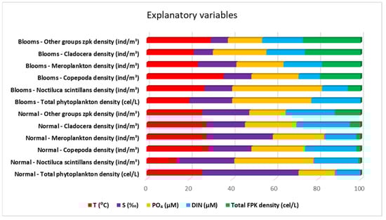
Figure 8.
The importance of explanatory variables from the Machine Learning—Forest-based Classification and Regression algorithm models for the Romanian Black Sea coast ecosystem, 2008–2018, warm season.
Similar to previous research findings documented by Lomartire et al. [45], it has been observed that the overall density of phytoplankton exerts a limited influence on the proliferation of nonfodder zooplankton, such as N. scintillans. However, it facilitates the prevalence of “other groups” and cladocerans, especially during expansive bloom occurrences.
3.3. Working Hypotheses for Future Research on Planktonic Proliferations in the Romanian Area of the Black Sea
Taking into account the above, we developed and run two scenarios (which do not take into account the socio-economic development aspects of the area) to predict the development of the pelagic biological components (phytoplankton and zooplankton) in the warm season over the next 20 years (2042):
- The BAU (Business As Usual) scenario in which the variables behave as they did during the study period—temperature increases by 0.4 °C, salinity increases by 0.84‰, and nutrient concentrations remain constant.
- The scenario corresponding to RCP2.6, the “mildest” climate warming scenario, in which sea water temperature increases by 0.8 °C by 2050 [46]. Associated with this increase, we consider an increase in salinity by 1.68‰. Given that such a scenario envisages environmental protection measures and emission reduction, nutrient concentrations could also be reduced by 25% for phosphates and 70% for inorganic nitrogen [47].
For the dinoflagellate N. scintillans, it is observed that in both scenarios, high densities of the species are reached (with extreme values in scenario 2, which exceed scenario 1 by approximately 70%), characteristic of a eutrophic ecosystem which means that the climate change effects might encompass nutrients reduction (Figure 9).
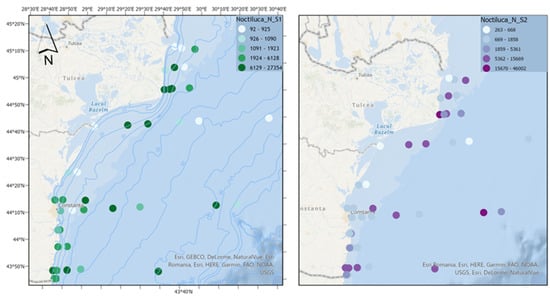
Figure 9.
The density of N. scintillans in scenarios 1 (BAU) (left) and 2 (RCP2.6) (right)—ML prediction for the warm season (2042).
Spatial analysis indicates that in scenario 1, lacking nutrient reduction strategies, elevated abundances are observed in the coastal region. However, in scenario 2, marked by substantial nutrient reduction efforts amidst amplified climate change impacts, nonfodder zooplankton displays comparable abundance levels in the coastal area and heightened values offshore. This shift potentially introduces imbalances, underscoring the critical significance of reducing nutrients in climate change scenarios.
Copepods, a major component of marine zooplankton, are the main food source of fish larvae [48], favoring the survival, growth, and development of juvenile fish [49]. It is observed that in the first scenario, copepods record optimal densities, which indicates a good trophic base for fish. The second scenario involves reaching much higher densities of copepods, which would lead to the development of more-than-favorable conditions of pelagic fish species, which prefer higher water temperatures (Figure 10).

Figure 10.
The density of copepods in scenarios 1 (BAU) (left) and 2 (RCP2.6) (right)—ML prediction for the warm season (2042).
Cladocerans are important components of food webs, consuming large amounts of microalgae and detritus, which, in turn, serve as food for copepods and larval and juvenile stages of fish [50]. In both scenarios, cladocerans reach high densities, indicating, in certain areas, a sustainable trophic base for higher trophic levels adapted to predicted temperature and salinity conditions (Figure 11).

Figure 11.
The density of cladocerans in scenarios 1 (BAU) (left) and 2 (RCP2.6) (right)—ML prediction for the warm season (2042).
Meroplankton can represent a substantial part of the zooplankton community, with its contributions to total density being greater in estuarine areas [51]. The main characteristic of shallow areas is the abundance of meroplankton organisms, which can produce real explosions in the water mass, constituting the dominant elements in zooplankton composition [52]. In the two scenarios, the meroplanktonic component reaches similar density values (Figure 12). It can compete for resources with holoplanktonic species and serves as a food source for planktonic predators [53]. On the other hand, climate change can affect the reproduction and recruitment of benthic invertebrates, affecting the abundance of meroplankton [54].

Figure 12.
The density of meroplankton in scenarios 1 (BAU) (left) and 2 (RCP2.6) (right)—ML prediction for the warm season (2042).
The category “other groups” consists of the appendicular Oikopleura dioica, the chaetognath Parasagitta setosa, and the mysid Mesopodopsis slabberi, with the latter being much less represented and with a low frequency of occurrence. Appendicularians bridge the gap between small primary producers and higher trophic consumers, being important as food for fish larvae [55]. Parasagitta setosa can exert high predation pressure on copepods and thus compete with the food available for the larval stages of fish [56]. Scenario 2 experiences a significant increase in the density of the “other groups” category, in contrast to scenario 1, which shows minimal growth (Figure 13). The overall phytoplankton density primarily drives this difference.
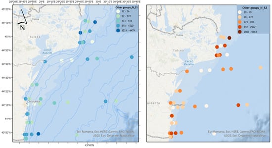
Figure 13.
The density of other groups in scenarios 1 (BAU) (left) and 2 (RCP2.6) (right)—ML prediction for the warm season (2042).
4. Discussion
The Black Sea, characterized by an average salinity of 17–18 g/L, exhibits a strong stratified nature, with distinct biogeochemical layers. The hydrographic regime is characterized by low-salinity surface waters of river origin overlying high-salinity deep waters of Mediterranean origin, with a sharp and permanent pycnocline found between. The pycnocline restricts the penetration of vertical mixing depth to 100–150 m. Its upper layer, the oxic layer, spans nearly 50 m and coincides with the euphotic zone and the pelagic habitat limit. It fosters active biological processes with high oxygen concentrations of about 300 µM, impacted by seasonal variations in nutrients and organic matter from rivers and coastal regions. The oxycline, signaling a sharp oxygen gradient, begins at 70–100 m depths in coastal zones. Below lies the suboxic layer, found at depths of 100–130 m, marked by low oxygen levels (<10 µM) and increasing hydrogen sulfide concentrations. Further down, the anoxic layer, starting at depths of 150–200 m, lacks oxygen, except for sustaining sulfate-reducing bacteria due to hydrogen sulfide [57,58,59].
Zooplankton is crucial for molding planktonic ecosystems, controlling phytoplankton growth, and transferring energy from lower-trophic animals to higher ones [60]. The local community structure is shaped by local environmental parameters, such as water temperature, pH, salinity, trophic state, or combinations of these factors (i.e., the species-sorting hypothesis) [61]. Furthermore, environmental nutrients significantly influence zooplankton [62,63], indirectly impacting zooplankton by having a top-down effect on phytoplankton [64].
Physico-chemical parameters are assessed to analyze the water quality and energy succession of an aquatic environment. The physico-chemical parameters of an aquatic ecosystem affect phytoplankton and zooplankton diversity and abundance [65]. A significant issue for the aquatic food web is the eutrophication caused by high phosphate and nitrate concentrations. Algal blooms prevent phytoplankton and other organisms from receiving enough oxygen, leading to an organism’s demise and to declining biodiversity and water body toxicity [66].
Thus, water temperature, salinity, and nutrient levels intricately shape zooplankton and phytoplankton dynamics within aquatic ecosystems. Temperature influences zooplankton metabolism and phytoplankton photosynthesis rates, impacting their growth and reproduction [67]. Salinity variations affect zooplankton distribution and phytoplankton osmoregulation, influencing community composition and species abundance [64,68]. Nutrient availability directly influences phytoplankton growth and zooplankton populations through food availability. These factors create complex trophic interactions, where changes in one component can cascade throughout the ecosystem, impacting higher trophic levels and overall ecosystem health. The interactions among these factors are often intertwined and non-linear. Changes in one parameter can have cascading effects throughout the entire ecosystem [68,69]. Understanding these mechanisms is critical for predicting and managing the responses of planktonic communities to environmental changes, aiding in the conservation and sustainable management of aquatic ecosystems. Integrated models that consider these interconnected factors are crucial for predicting and managing the responses of zooplankton/phytoplankton dynamics to environmental changes, ultimately preserving aquatic ecosystem stability and function [70].
Fuzzy-Logic Cognitive Mapping (FCM) was developed as early as 1986 to structure expert knowledge using a systems programming approach that is “fuzzy”, thought to be similar to how the human mind makes decisions. Because of their flexibility, FCMs were created to examine the perceptions of an environmental problem or to model a complex system with high uncertainty and little empirical data availability [40]. The model has 89 components and 203 linear connections (positive or negative (Table S2)) between them, connections that human thinking cannot make simultaneously to allow a precise analysis of the evolution of the pelagic component of the marine ecosystem, the concentrations of silicates and nitrates affecting the densities of meroplankton and copepods. Copepods are usually known as ammonium-excreting microorganisms; hence, positive associations between copepods and nitrite (NO2) and nitrate (NO3) have also been documented [71,72]. A comprehensive approach to improving water quality must consider the participation of many stakeholders in water management decisions [73,74,75,76,77,78,79], and FCMs are an important tool to show the connections between ecosystem components. The results obtained with FCM are further the basis of the system knowledge and the generation of hypotheses for the predictions in the different scenarios we developed based on the specialized literature.
In the next stage, based on the collected data and supervised machine learning (ML) algorithms from ArcGIS, we obtained the models and proliferation scenarios of phytoplankton and zooplankton, as indicators of eutrophication in the waters of the Romanian Black Sea coast. Zooplankton demonstrates a wide range of ecological strategies, dominance patterns, and effects on ecosystems in marine habitats. It is difficult and still early to adequately express this variation in conceptual and mathematical frameworks [44]. The advantage of ML over traditional statistical techniques, especially in earth sciences and ecology, is the ability to model numerous variables, which may be non-linear, with complex interactions between them and sometimes with missing values [80,81]. Few comparative studies have demonstrated that machine learning techniques surpass conventional statistical methods across a diverse range of challenges in the fields of earth sciences and ecology [82]. However, this requires careful analysis, so we created the semi-quantitative model based on FCM in the preliminary stage [81].
In both ML scenarios, high densities of N. scintillans were observed. This dinoflagellate impacts the ecosystem in coastal areas around the world [83], generally in the spring and summer seasons, when it registers high abundances, establishing the blooming phenomenon of species [84]. The blooms generated by N. scintillans are closely related to food availability, especially the presence of diatoms, which it consumes, controlling the dynamics of this phytoplankton group [72]. The phenomenon causes mortality among fish, many of which are of economic importance, as well as marine invertebrates, due to the accumulation of high ammonia levels in the water [85]. N. scintillans plays an essential role in marine food chains [84], feeding on a wide variety of organisms such as phytoplankton (mainly diatoms), eggs, larvae, and fecal pellets of crustaceans, as well as other mesozooplanktonic organisms [86]. High densities of this dinoflagellate can limit the local population growth of copepods, not only when they compete for food but also because they feed on their eggs and nauplii [87].
The scenarios run for copepods showed increased abundance, which can positively impact the environment, especially for pelagic fish. There is evidence that recruitment is highly dependent on copepod production [88]; high prey availability encourages recruitment and early survival by maximizing food intake and growth throughout the larval stage of life in the plankton [89]. These findings offer information regarding the presence of plankton prey, which can lead to a more efficient management decisions regarding fisheries. Although it is inconclusive to conclude that zooplankton biomass is the only factor affecting fish recruitment, high prey abundance available during fish spawning will promote recruitment [45]. Still, there remains a possibility that the increase in temperature could lead to a reduction in copepod species diversity and a shift toward smaller-sized copepod communities [90]. Additionally, another potential risk associated with copepods, the predominant zooplankton in oceans, involves their influence on seawater by introducing distinct polar lipids known as copepodamides. These lipids stimulate toxin production and bioluminescence in harmful dinoflagellates [91].
Meroplankton recorded similar abundance values in both scenarios. The ecological significance of planktonic larvae is two-fold: they are a dispersal stage for benthic organisms [92], determining the potential of benthic species to colonize adjacent habitats, and they can also constitute a significant portion of zooplankton [93], potentially competing for resources with holoplanktonic species and serving as a food source for planktonic predators [53,56]. Larval movement is a crucial biophysical mechanism in benthic ecosystems that, in advection-dominated environments, can result in a spatial decoupling between local community production and settlement [52].
The “other groups” category does not undergo an extensive development from a quantitative point of view, in contrast to scenario 2, where a much more significant increase in density is noted. Species belonging to this group act as a crucial link in the food chain between pico- and nanophytoplankton and larger zooplankton like fish larvae [94], copepods, ctenophores [95], and jellyfish [96]. P. setosa grows and matures at high copepod density and greater temperature, indicating that temperature and food are the main factors influencing P. setosa growth in the Black Sea [97], as observed in scenario 2.
Jellyfish and ctenophores, acting as predators of young fish and zooplankton, indicate ecosystem health decline or human-induced stress from overfishing and the reduction of zooplankton predators when they form blooms. This scenario might lead to an excessive presence of gelatinous zooplankton, causing a considerable adverse impact on fish recruitment [45]. The appearance of gelatinous zooplankton indirectly affects the ecosystem by boosting phytoplankton and detritus levels, consequently reducing water quality, triggering hypoxia, and causing harm to fish and other wildlife [98].
The nutritional quality of phytoplankton significantly influences the food web, primarily through its relationship with zooplankton. Therefore, to ensure efficient stock management and optimize fishing resources, it is crucial to consistently assess the trophic interactions among phytoplankton, zooplankton, and fish within fishery management practices [99]. Diminished future phytoplankton biomass will favor the development of gelatinous food webs. Hence, employing the trait-based modeling framework showcased here becomes a potent method for uncovering fresh perspectives on the impact of climate change on zooplankton and their crucial role in global marine ecosystems, effectively linking planktonic organisms with fish populations [100].
Elevated organic matter levels could potentially initiate alterations in the nitrogen-to-phosphorus ratio, significantly affecting the growth and diversity of phytoplankton and various marine algae. These imbalances might lead to shorter trophic food webs, reduced predator numbers, and potential decreases in biodiversity [101].
To prevent pollution in the ocean and govern the fishing sector to promote sustainable fishing, SDG 14, “Life Below Water”, seeks to safeguard marine ecosystems. The preservation and sustainable use of marine ecosystem services is, thus, the main driving force behind this goal [11,102]. The efficiency of conservation measures, their accompanying socio-economic benefits, and the relative contributions of land-based and ocean-based activities are all poorly understood from a scientific standpoint. There are still significant knowledge gaps in several areas of integrated coastal management. Furthermore, there is disagreement regarding the definition of ecosystem-based management. To ensure a successful implementation in managing marine activities, further research on cumulative consequences, the precautionary approach, and explicitly acknowledged trade-offs should be taken into account within such a framework [103]. Conservation efforts are nonetheless beset by issues related to capacity, rising rates of degradation of marine habitats, and a failure to use sustainable marine planning concepts. Stakeholder engagement and integration into decision-making processes still severely limits collaboration, information transfer, and the efficacy of compliance or monitoring initiatives, especially at the local level [104].
Understanding how the marine environment changes and affects ecosystems is crucial for achieving SDG 14 and other SDGs. Recent findings in the area indicated that numerous local stakeholders lack awareness of environmental challenges, as these are overshadowed by social and economic issues [105]. Still, at the national level, the commitment to SDGs exists [18], even though the efforts to build local, sustainable communities is generally low [106,107]. The promotion of sustainability across economic, social, and environmental activities requires the active involvement of national, regional, and local administrations, ensuring a cohesive approach. Alongside strategies and programs implemented at both European and national levels, local initiatives also contribute significantly. These initiatives, manifested through various projects, aim to realize sustainable development objectives. Beyond the broader goals of sustainable development, local policies specifically target meeting human needs and enhancing overall quality of life. However, the lack of continuity in national and local development programs introduces challenges, causing bottlenecks and disruptions in the pursuit of sustainable development goals [107]. As prospective future research, conducting an exploratory study to examine stakeholder views on sustainable development of the coastal community in the context of climate change can influence the development of strategies and policies that align more closely with their expectations, fostering inclusivity and effectiveness in sustainable development endeavors [108]. This exploration would not only contribute to academic insights into the dynamics of coastal community sustainable development but also provide practical inputs for the implementation of policies that resonate with the varied needs and aspirations of stakeholders [109].
Thus, to effectively mitigate the impact of climate change on marine ecosystems, we advocate for a comprehensive approach extending beyond climate issues. For instance, strengthening the resilience of zooplankton communities against climate effects necessitates adopting innovative methods, such as refining farming practices to reduce nutrient inputs. Unlike climate change, this non-climate stressor can be promptly managed through policy adjustments and improved management practices at national and regional levels. The results represent the spatial and temporal assessment and ecosystem modeling of the ecosystem services underpinning the Blue Economy, aligning with Sustainable Development Goal 14. The research emphasizes the urgent need to mitigate human-induced changes in marine ecosystems, shedding light on potential ecosystem changes by 2042 and providing valuable insights for guiding sustainable management practices globally.
This approach exemplifies the need and urgency to understand nutrient sources and concentrations and make nutrient management decisions based on scientific evidence aligned with achieving Sustainable Development Goal (UN) 14 (Aquatic Life)—the conservation and sustainable use of oceans, seas, and marine resources. It creates unique prediction models that explicitly include features and related trade-offs and then uses these qualities to describe and forecast zooplankton community structure and dynamics in various environmental contexts, including those involving possible futures with global climatic change [44]. Thus, the possibility of reaching the SDG goals is increased by filling knowledge and implementation gaps and better utilizing evidence based on science to guide policy formulation and implementation [110].
However, inherent limitations must be acknowledged. Challenges include potential data inadequacies impacting model accuracy, the complexity introduced by combining diverse modeling approaches, the need for careful algorithm selection and tuning, and the difficulty in generalizing predictions to unforeseen scenarios. Additionally, capturing the intricate dynamics of anthropogenic impacts, considering spatial variability, and addressing ethical considerations are vital aspects that require careful attention.
5. Conclusions
Understanding how the marine environment changes and affects ecosystems is crucial to achieving SDG 14—Life below Water. This study contributes to understanding how abiotic factors impact marine ecosystems, specifically focusing on the interactions between environmental parameters and the first two trophic levels for plankton in the Black Sea in two climate change scenarios combined with nutrient management policies. The research highlighted significant relationships by examining the influence of temperature, salinity, and nutrients on plankton over a decade during the warm season. Water temperature is a key driver affecting copepods and other groups of zooplankton densities, underscoring their potential vulnerability to temperature changes. Conversely, salinity fluctuations notably influence typical phytoplankton proliferation, primarily driven by phosphate concentrations. Despite these impacts, the study finds a surprising resilience of N. scintillans blooms to observed abiotic changes, raising questions about the resilience of certain species to environmental shifts. Moreover, the research provides predictive models using fuzzy cognitive maps (FCMs) and machine learning (ML) algorithms to forecast zooplankton growth under varying future scenarios, shedding light on potential ecosystem changes by 2042. Thus, to effectively mitigate climate change’s impact on marine ecosystems, we adopted a comprehensive approach beyond focusing solely on climate issues, e.g., on nutrients reduction policies. Strengthening the resilience of zooplankton communities against climate effects requires developing novel methods to minimize nutrients input by various sources. Unlike climate change, this non-climate stressor can be promptly managed through policy adjustments and improved management practices at national and regional levels [111]. Urgent attention is needed for integrated research that evaluates management solutions capable of addressing the combined impact of climate change and other human-induced pressures like the introduction of nutrients [112].
The implications of this research extend to addressing Sustainable Development Goals (SDGs) related to Life Below Water by emphasizing the urgent need to mitigate human-induced changes in marine ecosystems. The study’s findings highlight the ramifications of altered abiotic factors on ecosystem health, particularly regarding the potential for a eutrophic ecosystem.
Future research directions might encompass more extended and comprehensive monitoring to capture long-term trends, refining models to integrate socio-economic aspects and policy implications, and exploring mitigation strategies to counteract the adverse effects observed, such as eutrophication.
Supplementary Materials
The following supporting information can be downloaded at: https://www.mdpi.com/article/10.3390/su16051849/s1, Table S1: Descriptive statistics of physico-chemical parameters, nutrients, phytoplankton, and zooplankton—warm season, 2008–2018. Table S2: Correlations between physico-chemical parameters, nutrients, phytoplankton species, and zooplankton group density—warm season, 2008–2018. Table S3: Correlations between physico-chemical parameters, nutrients, phytoplankton total density, and zooplankton group density—warm season, 2008–2018.
Author Contributions
Conceptualisation, L.L. and E.B.; methodology, L.L. and E.B.; software, L.L.; validation, L.L. and E.B.; formal analysis, L.L. and E.B.; investigation, L.L. and E.B.; resources, L.L., L.B., E.P., F.T., O.V. and E.B.; data curation, L.L., L.B., E.P., F.T., O.V. and E.B.; writing—original draft preparation, L.L. and E.B.; writing—review and editing, L.L., L.B., E.P., F.T., O.V. and E.B; visualization, L.L., L.B., E.P., F.T., O.V. and E.B.; supervision, L.L. and E.B; project administration, L.L. and E.B; funding acquisition, E.B. All authors have read and agreed to the published version of the manuscript.
Funding
This research was funded by the Nucleu Programme INTELMAR 2019–2022 funded by Ministry of Research, Innovation and Digitization, grant number 45N/2019, project PN 19260202. This manuscript is a result of GES4SEAS (Achieving Good Environmental Status for maintaining ecosystem services, by assessing integrated impacts of cumulative pressures) project, funded by the European Union under the Horizon Europe program (grant agreement No. 101059877) (www.ges4seas.eu, accessed on 4 December 2023).
Data Availability Statement
The data belong to the National Institute for Marine Research and Development “Grigore Antipa” (NIMRD) and can be accessed by request at http://www.nodc.ro/data_policy_nimrd.php, accessed on 5 December 2023.
Conflicts of Interest
The authors declare no conflicts of interest. The funders had no role in the de-sign of the study; in the collection, analyses, or interpretation of data; in the writing of the manuscript; or in the decision to publish the results.
References
- Talukder, B.; Ganguli, N.; Matthew, R.; Vanloon, G.W.; Hipel, K.W.; Orbinski, J. Climate Change-Accelerated Ocean Biodiversity Loss & Associated Planetary Health Impacts. J. Clim. Chang. Health 2022, 6, 100114. [Google Scholar] [CrossRef]
- Hilmi, N.; Chami, R.; Sutherland, M.D.; Hall-Spencer, J.M.; Lebleu, L.; Benitez, M.B.; Levin, L.A. The Role of Blue Carbon in Climate Change Mitigation and Carbon Stock Conservation. Front. Clim. 2021, 3, 710546. [Google Scholar] [CrossRef]
- Franke, A.; Blenckner, T.; Duarte, C.M.; Ott, K.; Fleming, L.E.; Antia, A.; Reusch, T.B.; Bertram, C.; Hein, J.; Kronfeld-Goharani, U.; et al. Operationalizing Ocean Health: Toward Integrated Research on Ocean Health and Recovery to Achieve Ocean Sustainability. One Earth 2020, 2, 557–565. [Google Scholar] [CrossRef]
- Couespel, D.; Lévy, M.; Bopp, L. Oceanic Primary Production Decline Halved in Eddy-Resolving Simulations of Global Warming. Biogeosciences 2021, 18, 4321–4349. [Google Scholar] [CrossRef]
- du Pontavice, H.; Gascuel, D.; Kay, S.; Cheung, W. Climate-Induced Changes in Ocean Productivity and Food-Web Functioning Are Projected to Markedly Affect European Fisheries Catch. Mar. Ecol. Prog. Ser. 2023, 713, 21–37. [Google Scholar] [CrossRef]
- Hall-Spencer, J.M.; Harvey, B.P. Ocean Acidification Impacts on Coastal Ecosystem Services Due to Habitat Degradation. Emerg. Top Life Sci. 2019, 3, 197–206. [Google Scholar] [CrossRef] [PubMed]
- Haas, B.; Mackay, M.; Novaglio, C.; Fullbrook, L.; Murunga, M.; Sbrocchi, C.; McDonald, J.; McCormack, P.C.; Alexander, K.; Fudge, M.; et al. The Future of Ocean Governance. Rev. Fish Biol. Fish. 2022, 32, 253–270. [Google Scholar] [CrossRef] [PubMed]
- Johansen, D.F.; Vestvik, R.A. The Cost of Saving Our Ocean—Estimating the Funding Gap of Sustainable Development Goal 14. Mar. Policy 2020, 112, 103783. [Google Scholar] [CrossRef]
- Stead, S.M. Rethinking Marine Resource Governance for the United Nations Sustainable Development Goals. Curr. Opin. Environ. Sustain. 2018, 34, 54–61. [Google Scholar] [CrossRef]
- Diz, D.; Morgera, E.; Wilson, M. Marine Policy Special Issue: SDG Synergies for Sustainable Fisheries and Poverty Alleviation. Mar. Policy 2019, 110, 102860. [Google Scholar] [CrossRef]
- Gulseven, O. Measuring Achievements towards SDG 14, Life below Water, in the United Arab Emirates. Mar. Policy 2020, 117, 103972. [Google Scholar] [CrossRef]
- Sturesson, A.; Weitz, N.; Persson, Å. Stockholm Environment Institute SDG 14 Life below Water—A Review of Research Needs 1 1 SDG 14: Life below Water A Review of Research Needs Annex to the Formas Report Forskning för Agenda 2030: Översikt Av Forskningsbehov Och Vägar Framåt; Swedish Research Council for Sustainable Development: Stockholm, Sweden, 2018. [Google Scholar]
- Molony, B.W.; Ford, A.T.; Sequeira, A.M.M.; Borja, A.; Zivian, A.M.; Robinson, C.; Lønborg, C.; Escobar-Briones, E.G.; Di Lorenzo, E.; Andersen, J.H.; et al. Editorial: Sustainable Development Goal 14—Life Below Water: Towards a Sustainable Ocean. Front. Mar. Sci. 2022, 8, 829610. [Google Scholar] [CrossRef]
- Haward, M.; Haas, B. The Need for Social Considerations in SDG 14. Front. Mar. Sci. 2021, 8, 632282. [Google Scholar] [CrossRef]
- International Council for Science. A Guide to SDG Interactions: From Science to Implementation; International Council for Science: Paris, France, 2017. [Google Scholar]
- Schmidt, S.; Neumann, B.; Waweru, Y.; Durussel, C.; Unger, S.; Visbeck, M. SDG 14-conserve and sustainable use the oceans, seas and marine resources for sustainable development. In A Guide to SDG Interactions: From Science to Implementation; International Council for Science (ICSU): Paris, France, 2017. [Google Scholar]
- Lubchenco, J.; Camp, E.F.; Vargas, C.A.; Belhabib, D.; Anna, Z.; Amon, D.J.; Metaxas, A.; Harden-Davies, H. Priorities for progress towards Sustainable Development Goal 14 ‘Life below water’. Nat. Ecol. Evol. 2023, 7, 1564–1569. [Google Scholar] [CrossRef] [PubMed]
- Firoiu, D.; Ionescu, G.H.; Băndoi, A.; Florea, N.M.; Jianu, E. Achieving Sustainable Development Goals (SDG): Implementation of the 2030 Agenda in Romania. Sustainability 2019, 11, 2156. [Google Scholar] [CrossRef]
- Asadikia, A.; Rajabifard, A.; Kalantari, M. Systematic Prioritisation of SDGs: Machine Learning Approach. World Dev. 2021, 140, 105269. [Google Scholar] [CrossRef]
- Benedetti, F.; Vogt, M.; Elizondo, U.H.; Righetti, D.; Zimmermann, N.E.; Gruber, N. Major Restructuring of Marine Plankton Assemblages under Global Warming. Nat. Commun. 2021, 12, 5226. [Google Scholar] [CrossRef] [PubMed]
- Stocker, T.F. The Silent Services of the World Ocean. Science 2015, 350, 764–765. [Google Scholar] [CrossRef]
- Barbier, E.B. Marine Ecosystem Services. Curr. Biol. 2017, 27, R507–R510. [Google Scholar] [CrossRef]
- European Commission, Directorate-General for Maritime Affairs and Fisheries, Joint Research Centre. The EU Blue Economy Report 2021: Annexes; Publications Office of the European Union: Luxembourg, 2021. [Google Scholar] [CrossRef]
- Oguz, T.; Velikova, V. Abrupt Transition of the Northwestern Black Sea Shelf Ecosystem from a Eutrophic to an Alternative Pristine State. Mar. Ecol. Prog. Ser. 2010, 405, 231–242. [Google Scholar] [CrossRef]
- McQuatters-Gollop, A.; Mee, L.D.; Raitsos, D.E.; Shapiro, G.I. Non-Linearities, Regime Shifts and Recovery: The Recent Influence of Climate on Black Sea Chlorophyll. J. Mar. Syst. 2008, 74, 649–658. [Google Scholar] [CrossRef]
- Daskalov, G.M.; Boicenco, L.; Grishin, A.N.; Lazar, L.; Mihneva, V.; Shlyakhov, V.A.; Zengin, M. Architecture of Collapse: Regime Shift and Recovery in an Hierarchically Structured Marine Ecosystem. Glob. Chang. Biol. 2017, 23, 1486–1498. [Google Scholar] [CrossRef]
- Singh, K.S.; Gill, S.S.; The Combination between Machine Learning and Sustainable Development Goal (SDG). Insights2Techinfo. 2022. Available online: https://insights2techinfo.com/the-combination-between-machine-learning-and-sustainable-development-goal-sdg/ (accessed on 6 December 2023).
- Vinuesa, R.; Azizpour, H.; Leite, I.; Balaam, M.; Dignum, V.; Domisch, S.; Felländer, A.; Langhans, S.D.; Tegmark, M.; Nerini, F.F. The Role of Artificial Intelligence in Achieving the Sustainable Development Goals. Nat. Commun. 2020, 11, 233. [Google Scholar] [CrossRef] [PubMed]
- Frey, U.J. Putting Machine Learning to Use in Natural Resource Management—Improving Model Performance. Ecol. Soc. 2020, 25, art45. [Google Scholar] [CrossRef]
- Stupariu, M.-S.; Cushman, S.A.; Pleşoianu, A.-I.; Pătru-Stupariu, I.; Fürst, C. Machine Learning in Landscape Ecological Analysis: A Review of Recent Approaches. Landsc. Ecol. 2022, 37, 1227–1250. [Google Scholar] [CrossRef]
- Drogkoula, M.; Kokkinos, K.; Samaras, N. A Comprehensive Survey of Machine Learning Methodologies with Emphasis in Water Resources Management. Appl. Sci. 2023, 13, 12147. [Google Scholar] [CrossRef]
- Pugliese, R.; Regondi, S.; Marini, R. Machine Learning-Based Approach: Global Trends, Research Directions, and Regulatory Standpoints. J. Inf. Technol. Data Manag. 2021, 4, 19–29. [Google Scholar] [CrossRef]
- Goralski, M.A.; Tan, T.K. Artificial Intelligence and Sustainable Development. Int. J. Manag. Educ. 2020, 18, 100330. [Google Scholar] [CrossRef]
- Roy, D.K.; Munmun, T.H.; Paul, C.R.; Haque, M.P.; Al-Ansari, N.; Mattar, M.A. Improving Forecasting Accuracy of Multi-Scale Groundwater Level Fluctuations Using a Heterogeneous Ensemble of Machine Learning Algorithms. Water 2023, 15, 3624. [Google Scholar] [CrossRef]
- Papageorgiou, E.I.; Hatwágner, M.F.; Buruzs, A.; Kóczy, L.T. A Concept Reduction Approach for Fuzzy Cognitive Map Models in Decision Making and Management. Neurocomputing 2017, 232, 16–33. [Google Scholar] [CrossRef]
- Moncheva, S.; Parr, B.; Sarayi, D.; Hareket, I.I. Manual for Phytoplankton Sampling and Analysis in the Black Sea; Phytoplankton Manual, UP-GRADE Black Sea Scene Project, FP7 (226592); Black Sea Commission: Istanbul, Turkey, 2010. [Google Scholar]
- Alexandrov, B.; Arashkevich, E.; Gubanova, A.; Korshenko, A. Manual for Mesozooplankton Sampling and Analysis in the BlackSea Monitoring; Black Sea Commission: Istanbul, Turkey, 2014. [Google Scholar]
- Grasshoff, K.; Kremling, K.; Ehrhardt, M. Methods of Seawater Analysis, 3rd ed.; Grasshoff, K., Kremling, K., Ehrhardt, M., Eds.; Willey-VCH: Weinheim: Germany, 1999. [Google Scholar]
- TIBCO Software, Inc. TIBCO Statistica, Version 14.0.1.25; TIBCO Software, Inc.: Palo Alto, CA, USA, 2023. [Google Scholar]
- Gray, S.A.; Gray, S.; Cox, L.J.; Henly-Shepard, S. Mental Modeler: A Fuzzy-Logic Cognitive Mapping Modeling Tool for Adaptive Environmental Management. In Proceedings of the 2013 46th Hawaii International Conference on System Sciences (HICSS), Maui, HI, USA, 7–10 January 2013; pp. 965–973. [Google Scholar]
- ESRI. ArcGIS Desktop, Version 10.7; Environmental Systems Research Institute: Redlands, CA, USA, 2019. [Google Scholar]
- Breiman, L. Random Forests. Mach. Learn. 2001, 45, 5–32. [Google Scholar] [CrossRef]
- Calbet, A. The Trophic Roles of Microzooplankton in Marine Systems. ICES J. Mar. Sci. 2008, 65, 325–331. [Google Scholar] [CrossRef]
- Litchman, E.; Ohman, M.D.; Kiørboe, T. Trait-Based Approaches to Zooplankton Communities. J. Plankton Res. 2013, 35, 473–484. [Google Scholar] [CrossRef]
- Lomartire, S.; Marques, J.C.; Gonçalves, A.M. The Key Role of Zooplankton in Ecosystem Services: A Perspective of Interaction between Zooplankton and Fish Recruitment. Ecol. Indic. 2021, 129, 107867. [Google Scholar] [CrossRef]
- Genner, M.J.; Freer, J.J.; Rutterford, L.A. Future of the Sea: Biological Responses to Ocean Warming—Foresight Future of the Sea project, 2017, 30. Available online: https://assets.publishing.service.gov.uk/media/5a82cfefed915d74e3403b2a/Ocean_warming_final.pdf (accessed on 6 December 2023).
- Lazăr, L.; Boicenco, L.; Marin, O.; Culcea, O.; Pantea, E.; Bișinicu, E.; Timofte, F.; Abaza, V.; Spînu, A. Black Sea Eutrophication Status—The Integrated Assessment Limitations and Obstacles. Rev. Cercet. Mar. Rev. Rech. Mar. Mar. Res. J. 2019, 49, 57–73. [Google Scholar]
- Poulet, S.A.; Williams, R.; Conway, D.V.P.; Videau, C. Co-Occurrence of Copepods and Dissolved Free Amino Acids in Shelf Sea Waters. Mar. Biol. 1991, 108, 373–385. [Google Scholar] [CrossRef]
- Hansen, B.W. Advances Using Copepods in Aquaculture. J. Plankton Res. 2017, 39, 972–974. [Google Scholar] [CrossRef]
- Havel, J.E. Cladocera. In Encyclopedia of Inland Waters; Elsevier: Amsterdam, The Netherlands, 2009; pp. 611–622. [Google Scholar] [CrossRef]
- Stübner, E.I.; Søreide, J.E.; Reigstad, M.; Marquardt, M.; Blachowiak-Samolyk, K. Year-Round Meroplankton Dynamics in High-Arctic Svalbard. J. Plankton Res. 2016, 38, 522–536. [Google Scholar] [CrossRef]
- Ershova, E.A.; Descoteaux, R.; Wangensteen, O.S.; Iken, K.; Hopcroft, R.R.; Smoot, C.; Grebmeier, J.M.; Bluhm, B.A. Diversity and Distribution of Meroplanktonic Larvae in the Pacific Arctic and Connectivity with Adult Benthic Invertebrate Communities. Front. Mar. Sci. 2019, 6, 490. [Google Scholar] [CrossRef]
- Short, J.; Metaxas, A.; Daigle, R.M. Predation of Larval Benthic Invertebrates in St George’s Bay, Nova Scotia. J. Mar. Biol. Assoc. United Kingd. 2013, 93, 591–599. [Google Scholar] [CrossRef]
- Birchenough, S.N.; Reiss, H.; Degraer, S.; Mieszkowska, N.; Borja, Á.; Buhl-Mortensen, L.; Braeckman, U.; Craeymeersch, J.; De Mesel, I.; Kerckhof, F.; et al. Climate Change and Marine Benthos: A Review of Existing Research and Future Directions in the North Atlantic. WIREs Clim. Chang. 2015, 6, 203–223. [Google Scholar] [CrossRef]
- Gorsky, G.; Fenaux, R. The Role of Appendicularia in Marine Food Webs. In The biology of Pelagic Tunicates; Oxford University Press: Oxford, UK, 1998; pp. 161–169. [Google Scholar]
- Samemoto, D.D. Vertical Distribution and Ecological Significance of Chaetognaths in the Arctic Environment of Baffin Bay. Polar Biol. 1987, 7, 317–328. [Google Scholar] [CrossRef]
- Magliozzi, C.; Palma, M.; Druon, J.-N.; Palialexis, A.; Abigail, M.-G.; Ioanna, V.; Rafael, G.Q.; Elena, G.; Birgit, H.; Laura, B.; et al. Status of Pelagic Habitats within the EU-Marine Strategy Framework Directive: Proposals for Improving Consistency and Representativeness of the Assessment. Mar. Policy 2023, 148, 105467. [Google Scholar] [CrossRef]
- Temel Oguz. State of the Environment of the Black Sea (2001–2006/7); Oguz, T., Ed.; Publications of the Commission on the Protection of the Black Sea Against Pollution (BSC): Istanbul, Turkey, 2008. [Google Scholar]
- Konovalov, S.K.; Murray, J.W. Variations in the Chemistry of the Black Sea on a Time Scale of Decades 1960–1995; Elsevier: Amsterdam, The Netherlands, 2001; Volume 31, Available online: https://www.elsevier.comrlocaterjmarsys (accessed on 1 November 2023).
- Sun, Y.; Li, H.; Yang, Q.; Liu, Y.; Fan, J.; Guo, H. Disentangling Effects of River Inflow and Marine Diffusion in Shaping the Planktonic Communities in a Heavily Polluted Estuary. Environ. Pollut. 2020, 267, 115414. [Google Scholar] [CrossRef]
- Xiong, W.; Li, J.; Chen, Y.; Shan, B.; Wang, W.; Zhan, A. Determinants of Community Structure of Zooplankton in Heavily Polluted River Ecosystems. Sci. Rep. 2016, 6, 22043. [Google Scholar] [CrossRef]
- Santangelo, J.M.; Bozelli, R.L.; Rocha, A.d.M.; Esteves, F.d.A. Effects of Slight Salinity Increases on Moina micrura (Cladocera) Populations: Field and Laboratory Observations. Mar. Freshw. Res. 2008, 59, 808. [Google Scholar] [CrossRef]
- Sun, X.; Zhang, H.; Wang, Z.; Huang, T.; Huang, H. Phytoplankton Community Response to Environmental Factors along a Salinity Gradient in a Seagoing River, Tianjin, China. Microorganisms 2022, 11, 75. [Google Scholar] [CrossRef] [PubMed]
- Sun, X.; Zhang, H.; Wang, Z.; Huang, T.; Tian, W.; Huang, H. Responses of Zooplankton Community Pattern to Environmental Factors along the Salinity Gradient in a Seagoing River in Tianjin, China. Microorganisms 2023, 11, 1638. [Google Scholar] [CrossRef] [PubMed]
- Oparaku, N.F.; Andong, F.A.; Nnachi, I.A.; Okwuonu, E.S.; Ezeukwu, J.C.; Ndefo, J.C. The Effect of Physicochemical Parameters on the Abundance of Zooplankton of River Adada, Enugu, Nigeria. J. Freshw. Ecol. 2022, 37, 33–56. [Google Scholar] [CrossRef]
- Gokhale, G.; Dutt Sharma, G. Impact of Abiotic Stress on Phytoplankton and Zooplankton with Special Reference to Food Web. In Advances in Plant Defense Mechanisms; IntechOpen: London, UK, 2022. [Google Scholar] [CrossRef]
- Zhao, Q.; Liu, S.; Niu, X. Effect of Water Temperature on the Dynamic Behavior of Phytoplankton–Zooplankton Model. Appl. Math. Comput. 2020, 378, 125211. [Google Scholar] [CrossRef]
- Zadereev, E.; Drobotov, A.; Anishchenko, O.; Kolmakova, A.; Lopatina, T.; Oskina, N.; Tolomeev, A. The Structuring Effects of Salinity and Nutrient Status on Zooplankton Communities and Trophic Structure in Siberian Lakes. Water 2022, 14, 1468. [Google Scholar] [CrossRef]
- Wei, Y.; Ding, D.; Gu, T.; Jiang, T.; Qu, K.; Sun, J.; Cui, Z. Different Responses of Phytoplankton and Zooplankton Communities to Current Changing Coastal Environments. Environ. Res. 2022, 215, 114426. [Google Scholar] [CrossRef] [PubMed]
- Acevedo-Trejos, E.; Cadier, M.; Chakraborty, S.; Chen, B.; Cheung, S.Y.; Grigoratou, M.; Guill, C.; Hassenrück, C.; Kerimoglu, O.; Klauschies, T.; et al. Modelling Approaches for Capturing Plankton Diversity (MODIV), Their Societal Applications and Data Needs. Front. Mar. Sci. 2022, 9, 975414. [Google Scholar] [CrossRef]
- Le Borgne, R. The Release of Soluble End Products of Metabolism. In The Biological Chemistry of Marine Copepods; Corner, E.D.S., O’Hara, S.C.M., Eds.; Oxford University Press: New York, NY, USA, 1986; pp. 109–164. [Google Scholar]
- Bișinicu, E.; Abaza, V.; Cristea, V.; Harcotă, G.E.; Lazar, L.; Tabarcea, C.; Timofte, F. The Assessment of the Mesozooplankton Community from the Romanian Black Sea Waters and the Relationship to Environmental Factors. Cercet. Mar. Rech. Mar. 2021, 51, 108–128. [Google Scholar] [CrossRef]
- Fonseca, K.; Espitia, E.; Breuer, L.; Correa, A. Using Fuzzy Cognitive Maps to Promote Nature-Based Solutions for Water Quality Improvement in Developing-Country Communities. J. Clean. Prod. 2022, 377, 134246. [Google Scholar] [CrossRef]
- Zare, S.G.; Alipour, M.; Hafezi, M.; Stewart, R.A.; Rahman, A. Examining Wind Energy Deployment Pathways In Complex Macro-Economic and Political Settings Using a Fuzzy Cognitive Map-Based Method. Energy 2021, 238, 121673. [Google Scholar] [CrossRef]
- Giordano, R.; Pluchinotta, I.; Pagano, A.; Scrieciu, A.; Nanu, F. Enhancing Nature-Based Solutions Acceptance through Stakeholders’ Engagement in Co-Benefits Identification and Trade-Offs Analysis. Sci. Total. Environ. 2020, 713, 136552. [Google Scholar] [CrossRef] [PubMed]
- Grigg, N.S. Social Aspects of Water Management. In Integrated Water Resource Management; Palgrave Macmillan UK: London, UK, 2016; pp. 319–338. [Google Scholar] [CrossRef]
- Özesmi, U.; Özesmi, S.L. Ecological Models Based on People’s Knowledge: A Multi-Step Fuzzy Cognitive Mapping Approach. Ecol. Model. 2004, 176, 43–64. [Google Scholar] [CrossRef]
- Sansa, M.; Badreddine, A.; Romdhane, T. Ben. Sustainable Design Based on LCA and Operations Management Methods:SWOT, PESTEL, and 7S. In Methods in Sustainability Science; Elsevier: Amsterdam, The Netherlands, 2021; pp. 345–364. [Google Scholar] [CrossRef]
- Wilson, N.J.; Mutter, E.; Inkster, J.; Satterfield, T. Community-Based Monitoring as the Practice of Indigenous Governance: A Case Study of Indigenous-Led Water Quality Monitoring in the Yukon River Basin. J. Environ. Manag. 2018, 210, 290–298. [Google Scholar] [CrossRef]
- Recknagel, F. Applications of Machine Learning to Ecological Modelling. Ecol. Model. 2001, 146, 303–310. [Google Scholar] [CrossRef]
- Olden, J.D.; Lawler, J.J.; Poff, N.L. Machine Learning Methods without Tears: A Primer for Ecologists. Q. Rev. Biol. 2008, 83, 171–193. [Google Scholar] [CrossRef]
- Thessen, A. Adoption of Machine Learning Techniques in Ecology and Earth Science. One Ecosyst. 2016, 1, e8621. [Google Scholar] [CrossRef]
- Umani, S.F.; Beran, A.; Parlato, S.; Virgilio, D.; Zollet, T.; De Olazabal, A.; Lazzarini, B.; Cabrini, M. Noctiluca scintillans MACARTNEY in the Northern Adriatic Sea: Long-Term Dynamics, Relationships with Temperature and Eutrophication, and Role in the Food Web. J. Plankton Res. 2004, 26, 545–561. [Google Scholar] [CrossRef]
- Miyaguchi, H.; Fujiki, T.; Kikuchi, T.; Kuwahara, V.S.; Toda, T. Relationship between the Bloom of Noctiluca scintillans and Environmental Factors in the Coastal Waters of Sagami Bay, Japan. J. Plankton Res. 2006, 28, 313–324. [Google Scholar] [CrossRef]
- Tada, K.; Plthakpol, S.; Montani, S. Seasonal Variation in the Abundance of Noctiluca scintillans in the Seto Inland Sea, Japan. Plankton Biol. Ecol. 2004, 51, 7–14. [Google Scholar]
- Ollevier, A.; Mortelmans, J.; Aubert, A.; Deneudt, K.; Vandegehuchte, M.B. Noctiluca scintillans: Dynamics, Size Measurements and Relationships with Small Soft-Bodied Plankton in the Belgian Part of the North Sea. Front. Mar. Sci. 2021, 8, 777999. [Google Scholar] [CrossRef]
- Nakamura, Y. Biomass, Feeding and Production of Noctiluca scintillans in the Seto Inland Sea, Japan. J. Plankton Res. 1998, 20, 2213–2222. [Google Scholar] [CrossRef]
- Castonguay, M.; Plourde, S.; Robert, D.; Runge, J.A.; Fortier, L.; Ludsin, S.A.; DeVanna, K.M.; Smith, R.E.; Murphy, H.M.; Jenkins, G.P.; et al. Copepod Production Drives Recruitment in a Marine Fish. Can. J. Fish. Aquat. Sci. 2008, 65, 1528–1531. [Google Scholar] [CrossRef]
- Cushing, D. Plankton Production and Year-Class Strength in Fish Populations: An Update of the Match/Mismatch Hypothesis. In Advances in Marine Biology; Elsevier Applied Science Publishers Ltd.: London, UK, 1990; Volume 26, pp. 249–293. [Google Scholar] [CrossRef]
- Jiang, Z.-B.; Zeng, J.-N.; Chen, Q.-Z.; Huang, Y.-J.; Liao, Y.-B.; Xu, X.-Q.; Zheng, P. Potential Impact of Rising Seawater Temperature on Copepods Due to Coastal Power Plants in Subtropical Areas. J. Exp. Mar. Biol. Ecol. 2009, 368, 196–201. [Google Scholar] [CrossRef]
- Selander, E.; Berglund, E.C.; Engström, P.; Berggren, F.; Eklund, J.; Harðardóttir, S.; Lundholm, N.; Grebner, W.; Andersson, M.X. Copepods Drive Large-Scale Trait-Mediated Effects in Marine Plankton. Sci. Adv. 2019, 5, eaat5096. [Google Scholar] [CrossRef] [PubMed]
- Shanks, A.L. Pelagic Larval Duration and Dispersal Distance Revisited. Biol. Bull. 2009, 216, 373–385. [Google Scholar] [CrossRef] [PubMed]
- Gluchowska, M.; Kwasniewski, S.; Prominska, A.; Olszewska, A.; Goszczko, I.; Falk-Petersen, S.; Hop, H.; Weslawski, J.M. Zooplankton in Svalbard Fjords on the Atlantic–Arctic Boundary. Polar Biol. 2016, 39, 1785–1802. [Google Scholar] [CrossRef]
- Sakaguchi, K.; Varughese, A.; Auld, G. Climate Wars? A Systematic Review of Empirical Analyses on the Links between Climate Change and Violent Conflict. Int. Stud. Rev. 2017, 19, 622–645. [Google Scholar] [CrossRef]
- Shiganova, T.; Sommer, U.; Javidpour, J.; Molinero, J.; Malej, A.; Kazmin, A.; Isinibilir, M.; Christou, E.; Frangou, I.S.; Marambio, M.; et al. Patterns of Invasive Ctenophore Mnemiopsis leidyi Distribution and Variability in Different Recipient Environments of the Eurasian Seas: A Review. Mar. Environ. Res. 2019, 152, 104791. [Google Scholar] [CrossRef]
- Masunaga, A.; Liu, A.W.; Tan, Y.; Scott, A.; Luscombe, N.M. Streamlined Sampling and Cultivation of the Pelagic Cosmopolitan Larvacean, Oikopleura dioica. J. Vis. Exp. 2020, 16, e61279. [Google Scholar] [CrossRef]
- Mutlu, E. Diel Vertical Migration of Sagitta setosa as Inferred Acoustically in the Black Sea. Mar. Biol. 2006, 149, 573–584. [Google Scholar] [CrossRef]
- Daskalov, G.; Shlyakhov, V. Influence of Gelatinous Zooplankton on Fish Stocks in the Black Sea: Analysis of Biological Time-Series. Available online: https://www.researchgate.net/publication/37615302 (accessed on 30 October 2023).
- Waya, R.K.; Limbu, S.M.; Ngupula, G.W.; Mwita, C.J.; Mgaya, Y.D. Temporal Patterns in Phytoplankton, Zooplankton and Fish Composition, Abundance and Biomass in Shirati Bay, Lake Victoria, Tanzania. Lakes Reserv. Sci. Policy Manag. Sustain. Use 2017, 22, 19–42. [Google Scholar] [CrossRef]
- Heneghan, R.F.; Everett, J.D.; Blanchard, J.L.; Sykes, P.; Richardson, A.J. Climate-Driven Zooplankton Shifts Cause Large-Scale Declines in Food Quality for Fish. Nat. Clim. Chang. 2023, 13, 470–477. [Google Scholar] [CrossRef]
- Reichelt-Brushett, A. (Ed.) Marine Pollution-Monitoring, Management and Mitigation; Springer Nature: Cham, Switzerland, 2023. [Google Scholar]
- Ntona, M.; Morgera, E. Connecting SDG 14 with the Other Sustainable Development Goals through Marine Spatial Planning. Mar. Policy 2018, 93, 214–222. [Google Scholar] [CrossRef]
- Campbell, M.D.; Schoeman, D.S.; Venables, W.; Abu-Alhaija, R.; Batten, S.D.; Chiba, S.; Coman, F.; Davies, C.H.; Edwards, M.; Eriksen, R.S.; et al. Testing Bergmann’s Rule in Marine Copepods. Ecography 2021, 44, 1283–1295. [Google Scholar] [CrossRef]
- Koutouki, K.; Phillips, F.-K. SDG 14 on Ensuring Conservation and Sustainable Use of Oceans and Marine Resources: Contributions of International Law, Policy and Governance. SSRN Electron. J. 2023. [Google Scholar] [CrossRef]
- Lazar, L.; Rodino, S.; Pop, R.; Tiller, R.; D’haese, N.; Viaene, P.; De Kok, J.-L. Sustainable Development Scenarios in the Danube Delta—A Pilot Methodology for Decision Makers. Water 2022, 14, 3484. [Google Scholar] [CrossRef]
- Bercu, A.-M. The Sustainable Local Development in Romania—Key Issues for Heritage Sector. Procedia Soc. Behav. Sci. 2015, 188, 144–150. [Google Scholar] [CrossRef][Green Version]
- Davidescu, A.A.; Apostu, S.A.; Pantilie, A.M.; Amzuica, B.F. Romania’s South-Muntenia Region, towards Sustainable Regional Development. Implications for Regional Development Strategies. Sustainability 2020, 12, 5799. [Google Scholar] [CrossRef]
- Nonet, G.A.-H.; Gössling, T.; Van Tulder, R.; Bryson, J.M. Multi-Stakeholder Engagement for the Sustainable Development Goals: Introduction to the Special Issue. J. Bus. Ethics 2022, 180, 945–957. [Google Scholar] [CrossRef] [PubMed]
- Bal, M.; Bryde, D.; Fearon, D.; Ochieng, E. Stakeholder Engagement: Achieving Sustainability in the Construction Sector. Sustainability 2013, 5, 695–710. [Google Scholar] [CrossRef]
- von Schuckmann, K.; Holland, E.; Haugan, P.; Thomson, P. Ocean Science, Data, and Services for the UN 2030 Sustainable Development Goals. Mar. Policy 2020, 121, 104154. [Google Scholar] [CrossRef]
- Poloczanska, E.S.; Babcock, R.C.; Butler, A.; Hobday, A.J.; Hoegh-Guldberg, O.; Kunz, T.J.; Matear, R.; Milton, D.A.; Okey, T.A.; Richardson, A.J. Climate Change and Australian Marine Life. Oceanogr. Mar. Biol. 2007, 45, 407–478. [Google Scholar] [CrossRef]
- Richardson, A.J. In Hot Water: Zooplankton and Climate Change. ICES J. Mar. Sci. 2008, 65, 279–295. [Google Scholar] [CrossRef]
Disclaimer/Publisher’s Note: The statements, opinions and data contained in all publications are solely those of the individual author(s) and contributor(s) and not of MDPI and/or the editor(s). MDPI and/or the editor(s) disclaim responsibility for any injury to people or property resulting from any ideas, methods, instructions or products referred to in the content. |
© 2024 by the authors. Licensee MDPI, Basel, Switzerland. This article is an open access article distributed under the terms and conditions of the Creative Commons Attribution (CC BY) license (https://creativecommons.org/licenses/by/4.0/).