Abstract
One of the solutions to achieve the goal of net-zero emissions by 2050 is to try to reduce the carbon emission by using the carbon tax or carbon credit (carbon right). This paper examines the impact of carbon taxes and carbon credit costs on the cement industry, focusing on ESG indicators and corporate profits. Utilizing Activity-Based Costing and the Theory of Constraints, a production decision model is developed and analyzed using mathematical programming. The paper categorizes carbon tax models into continuous and discontinuous progressive tax rates, taking into account potential government policies like emission tax exemptions and carbon trading. It finds that reducing emission caps is more effective than increasing carbon tax rates in curbing emissions. These insights can assist governments in policy formulation and provide a reference framework for establishing carbon tax systems.
1. Introduction
In the context of rapid economic growth, the world is increasingly facing critical global challenges such as the greenhouse effect and environmental pollution. This scenario calls for holistic approaches to diminish environmental footprints, including strategies for reducing carbon emissions. In recent times, there has been a heightened focus from both consumers and governments on the environmental responsibilities of corporations [1]. The environmental consequences of corporate activities are now under intense scrutiny, greatly impacting their public image and reputation. Consequently, the integration of Environmental, Social, and Governance (ESG) practices within the changing business landscape has emerged as a paramount concern. Major corporations are actively engaging in the disclosure of ESG-related information, reflecting a commitment that goes beyond static objectives and towards dynamic, performance-based outcomes [2]. However, research is still lacking in providing specific decision support models for emission-intensive industries to comply with increasingly stringent environmental regulations worldwide.
The cement industry, similar to other high-temperature and energy-intensive sectors, is a significant source of carbon dioxide (CO2) emissions [3]. This is primarily due to fuel combustion used in the process. Additionally, the clinker production process, which involves the calcination of calcium carbonate (CaCO3) into calcium oxide (CaO) and CO2, releases a considerable amount of CO2. The emissions typically range from 0.85 to 1.35 tons per ton of clinker (Note: 1 ton = 1000 kg) [4,5,6]. Moreover, cement plants emit a variety of minor pollutants due to fuel combustion, including carbon monoxide (CO) and volatile organic pollutants, which are often categorized as total organic compounds (TOC), volatile organic compounds (VOC), or organic condensable particulate (OCP) [7]. Therefore, examining carbon tax and trading policy impacts on the cement industry is of great practical value and necessity.
This paper focuses on the cement industry to explore the impact of carbon taxes and carbon trading costs on ESG indicators and corporate profits. It examines the production processes in the cement industry, considering various carbon tax models and carbon trading mechanisms in relation to ESG indicators. The aim is to find the optimal product mix md study how carbon taxes and trading costs influence corporate profitability and product combinations. The study employs Activity-Based Costing (ABC) for accurate cost estimation and the Theory of Constraints (TOC) to identify and manage system limitations, thereby establishing a production decision model for businesses. The integrated ABC-TOC simulation model tailored to cement companies could serve as a decision framework for policymakers as well in designing mix-and-match carbon tax and trading schemes balancing environmental effectiveness and economic interests.
2. The Related References
2.1. The Related Researches for the Cement Industry
The carbon emissions from the cement industry can be quantitatively predicted using various mathematical and machine learning models. However, these models typically require multiple input factors, which can be challenging to acquire, leading to data uncertainty. To address this issue, some researchers have imposed strict conditions or enhanced model constraints to reduce uncertainty, aiming to improve prediction reliability.
Early efforts in this regard utilized the Long-range Energy Alternatives Planning System (LEAP) model [8] and were further refined with expert judgment [9]. Other effective models include the Stochastic Impacts by Regression on Population, Affluence, and Technology (STIRPAT) model [10], the Back Propagation Neural Network (BPNN) model [11,12], the Integrated MARKAL-EFOM System (TIMES) model for industry-level predictions [13,14], the Particle Swarm Optimization (PSO) algorithm [12,15], the system dynamic model [16], and the Verhulst Grey forecasting (V-GM) model for country-level predictions [17]. These studies emphasize the utility of these models and demonstrate relatively high levels of accuracy in their results.
However, it is worth noting that only a few studies have attempted to address data uncertainty issues by narrowing down the list of input factors, although most studies have pointed out that the selected factors primarily relate to energy efficiency and production in the cement industry [11,12,13,14,15,16,17].
2.2. Carbon Emissions, Carbon Tax, and Carbon Trading
A Carbon Tax transfers the external cost of carbon emissions to the emitters, effectively reducing emissions and helping achieve national carbon reduction goals [18,19]. Carbon trading, based on the Coase theorem, posits that with clearly defined property rights and minimal transaction costs, the market will allocate resources efficiently regardless of initial distribution [20]. By limiting national carbon emissions and assigning quotas to enterprises and organizations, those achieving carbon reduction can sell excess credits to others needing more. Over time, companies consistently buying credits will increase carbon reduction efforts due to high production costs, thereby decreasing their need and cost for additional credits, leading to overall emission reductions and achieving carbon reduction targets [18,20,21]. While the majority of existing literature focuses exclusively on the impact of carbon taxes, few studies have examined and compared the differential influences of various carbon tax systems along with carbon trading schemes in a holistic model tailored to specific industries. This remains an important research gap needing further investigation.
2.3. ESG Indicators in the Cement Industry
ESG (Environmental, Social, Governance) represents a modern way of assessing a company’s performance beyond financial metrics, encompassing its environmental impact, social responsibility, and corporate governance. Achieving high ESG scores is increasingly important for companies and investors, aiming for sustainable business practices [22,23].
This research showcases the cement corporation as a prime example of commitment to sustainability. Their strategic focus on “low-carbon cement, resource recycling, and green energy” is at the core of their business model [24]. By leveraging the high temperatures inherent in cement production, they effectively dispose of difficult-to-treat industrial and urban waste, fostering a cross-industry circular economy. They place a strong emphasis on replacing traditional cement raw materials and fuels with recycled alternatives, actively contributing to carbon reduction and the development of eco-friendly building materials. In addition, the corporation is making significant strides in renewable energy, investing in both generation and storage technologies. This aligns with their aspiration to achieve the 2050 net-zero emissions target, demonstrating a proactive approach in environmental stewardship and sustainability. However, more quantitative model-based analyses are still needed to provide strategic decision support for cement companies under various policy scenarios of carbon taxes and emissions trading schemes on the pathway towards net-zero goals.
2.4. Activity-Based Costing and Theory of Constraints
Activity-Based Costing (ABC) involves breaking down each product or service into its fundamental activities and then using cost tracing and allocation methods to calculate accurate costs [18,19]. This approach attributes operational costs to cost objects to provide reliable cost distribution information [18,19,25,26]. Many industries now consider not only direct and indirect operational costs but also external costs, including those related to suppliers, environmental protection [27], carbon emissions, and internal carbon pricing [28], to make more precise production decisions. It has been over 30 years since ABC was proposed [29], and ABC has been applied to various industries, non-profitable organizations, and governmental entities [30,31,32,33,34,35,36,37].
The Theory of Constraints (TOC), as outlined by Goldratt and Cox [38], revolves around the concept that all organizations encounter limitations due to resource constraints. Rather than viewing these constraints as weaknesses, TOC suggests they should be leveraged as benchmarks for enhancing production and operational efficiency [39,40]. This theory focuses on optimizing processes within the confines of these constraints to achieve maximum efficiency and utility [41]. Additionally, TOC offers a practical framework for organizations to determine the most effective product mix in uncertain environments [42]. It does this by identifying the key bottlenecks within processes and implementing strategies to manage or alleviate these constraints, thus facilitating smoother and more efficient operations.
Unlike traditional linear programming purely targeting profit maximization, this model leverages key concepts from ABC and TOC in its construction and solution. Specifically, ABC enables higher costing accuracy by allocating operational costs across various activities, as manifested in the incorporation of raw material, labor, and carbon emission costs into the objective function. Additionally, TOC provides guidance to identify the “system constraint” of carbon emission reduction quotas that direct production decisions rather than solely maximizing profit. This aligns with TOC’s notion of benchmarking efficiency improvements to constraints.
3. Research Methods
3.1. Cement Production Process and ESG Indicators
This representation in Figure 1 provides a comprehensive overview of the cement production process, highlighting each key stage: raw meal grinding (m = 1), calcination (m = 2), cement grinding (m = 3), and the three batching processes (m = 4, m = 5, m = 6). A notable innovation in this process is the integration of waste from other industries as alternative raw materials. Particularly during the calcination stage (m = 2), the high temperature, strong turbulence, and prolonged retention time effectively process the waste. The calcination yields useful by-products like sludge and slag, as well as essential elements such as silicon, aluminum, iron, and calcium, which are then recycled back into the production process. This strategy not only aids in waste management but also contributes to cost reduction, making the process more efficient and sustainable.
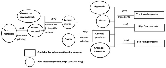
Figure 1.
Cement Production Process.
This study establishes specific objectives for the years 2023 to 2025, aimed at decreasing greenhouse gas emissions and improving resource recycling. The goals for greenhouse gas reduction, based on the 2016 baseline, are focused on CO2 emissions of cementitious material per ton. While the targets for 2023 and 2024 remain undefined, the ambition for 2025 is set at an 11% reduction. In terms of resource recycling, the study sets quantitative targets: 114 ten thousand tons in 2023, increased to 120 ten thousand tons in 2024, and further to 125 in 2025. These targets reflect a strategic move towards enhancing sustainability within the industry.
Key ESG indicators from the cement sustainability report are integrated into the study [24]. The emphasis is on reducing CO2 emissions and using alternative raw materials. The model applies the Theory of Constraints to systematically reduce CO2 emissions annually while increasing the use of alternative materials. This approach aims to align with environmental sustainability, reduce the carbon footprint, and improve resource efficiency, demonstrating a commitment to sustainable industrial practices.
3.2. Research Assumptions
This model sets 3 periods to simulate the evolution of corporate production decisions and profitability when facing more stringent emission reduction requirements over time. The 3-period model can reflect the gradual increases in emission reduction efforts and alternative material usage, as well as their impact on corporate profits. Theoretically, the model can be extended to encompass more periods to simulate and predict corporate decision-making behaviors over a longer time horizon. However, considering the complexity of parameters, it is appropriate to currently set it as 3 periods.
This study uses the cement industry as a case to examine the impact of carbon tax and carbon credit (carbon right) costs on ESG indicators and corporate profitability. By integrating Activity-Based Costing and the Theory of Constraints, a production decision model for the enterprise is established. Mathematical programming methods are then applied to explore the effects of carbon tax and carbon credit costs on ESG indicators and profit. To isolate external uncontrollable factors, the following assumptions are made:
- The company primarily produces four products: Cement finished product (i = 1), Traditional concrete (i = 2), High-fluidity concrete (i = 3), and Self-compacting concrete (i = 4), with unit prices remaining constant during production.
- Seven main raw materials are used: Clinker (j = 1), Gypsum (j = 2), alternative materials (j = 3), Cement (j = 4), Aggregates (j = 5), Water (j = 6), and Pyrite (j = 7), with material costs fixed throughout production.
- Waste from other industries is incorporated as alternative materials, for instance, sludge, slag, and elements like silicon, aluminum, iron, and calcium, which are then used as raw materials. This not only aids in waste treatment but also reduces costs.
- The usage of alternative materials is considered an ESG indicator for the company, with yearly increments aiming to achieve the “Net Zero Emissions by 2050” goal.
- During production, all steps are categorized into unit-level, batch-level, and product-level operations.
- According to regulations and policies, human resources may work overtime, but wages are calculated based on overtime rates. Additionally, the utilization rates of all machinery and labor are 100%, with no idle resources, and wage rates remain constant throughout production.
- Carbon tax is levied on the production of each unit of product, thus the tax amount depends on the quantity produced.
- The cap on carbon credit trading is limited by government regulations, assumed to be unchanged in the short term, and the trading costs of carbon credits for each company are zero.
- The ratio of carbon emission reduction (CO2 in tons/binder material in tons) is progressively increased yearly to meet the “Net Zero Emissions by 2050” target.
3.3. Objective Function
3.3.1. General Formula for the Objective Function
The objective is to maximize profit (π). This is calculated as the total revenue from cement and concrete sales minus the total costs, which include direct material costs, direct labor costs, batch-level operational costs, product-level operational costs, carbon emission costs, and fixed expenses. To maximize profit (π), the formula is defined as follows:
This objection function encapsulates the comprehensive cost structure and revenue streams within a cement and concrete business, taking into account various direct and indirect expenses as well as the environmental costs associated with carbon emissions. The goal is to optimize these variables to achieve the highest possible profit while maintaining operational efficiency and environmental compliance.
The general form of a multi-period objective function might be expressed as:
These definitions provide a structured framework for the mathematical modeling of the cement production process, taking into account various factors like product types, raw materials, production processes, and temporal dynamics.
| Maximization of profit | |
| i | Product index where i = 1 to 4. Products are: i = 1 (Finished Cement), i = 2 (Traditional Concrete), i = 3 (High Fluidity Concrete), i = 4 (Self-compacting Concrete). |
| j | Raw material index where j = 1 to 7. Raw materials are: j = 1 (Clinker), j = 2 (Gypsum), j = 3 (Alternative Materials), j = 4 (Cement), j = 5 (Aggregates), j = 6 (Water), j = 7 (Chemical Additives). |
| m | Process index where m = 1 to 6. Processes are: m = 1 (Raw Meal Grinding), m = 2 (Calcination), m = 3 (Cement Grinding), m = 4, m = 5, m = 6 (Batching). |
| t | Time period index where t = 1 to 3. |
| Unit price of the ith product for different time periods (t = 1, 2, 3). | |
| Quantity of the ith product in period t (i = 1~4; t = 1~3). | |
| Quantity of the jth raw material required for producing one unit of the ith product during the tth time period (i = 1~4; j = 1~7; t = 1~3). | |
| Total direct labor costs at points , and respectively. | |
| Non-negative variables for period t, with at most two adjacent variables being non-zero (t = 1~3). | |
| Unit batch-level cost in the mth process (m = 3~6). | |
| Resource consumption per batch for the ith product in the mth batch-level process (i = 1~4; m = 3~6). | |
| Number of batches for the ith product in the mth process during period t (i = 1~4; m = 3~6; t = 1~3). | |
| Number of batches for the ith product in the mth batch-level process (i = 1~4; m = 3~6). | |
| Unit product-level cost in the mth process (m = 3~6). | |
| Resource consumption for the ith product in the mth product-level process (i = 1~4; m = 3~6). | |
| Binary variable for period t, determining whether the ith product is produced (1 if produced, 0 otherwise) (i = 1~4; t = 1~3). | |
| Total fixed cost in period t (t = 1~3). |
3.3.2. Direct Material Cost Function
This study assumes cement producers primarily use seven raw materials: clinker (j = 1), gypsum (j = 2), alternative materials (j = 3), cement (j = 4), aggregates (j = 5), water (j = 6), and Pyrite (j = 7). In the multi-period model, the usage of alternative materials (j = 3) will be progressively increased each year to meet the ESG targets by 2025, with the direct costs of these materials factored into the profit function.
With constraints:
Symbol Definitions:
| Unit cost of the jth raw material, (j = 1~7) | |
| Quantity of the jth raw material required per unit of the ith product (i = 1~4; j = 1~7; t = 1~3) | |
| Upper limit on the available quantity of the jth raw material in period t (j = 1~7; t = 1~3) | |
| Lower limit on the available quantity of the jth raw material in period t (j = 3; t = 1~3) |
3.3.3. Direct Labor Cost Function
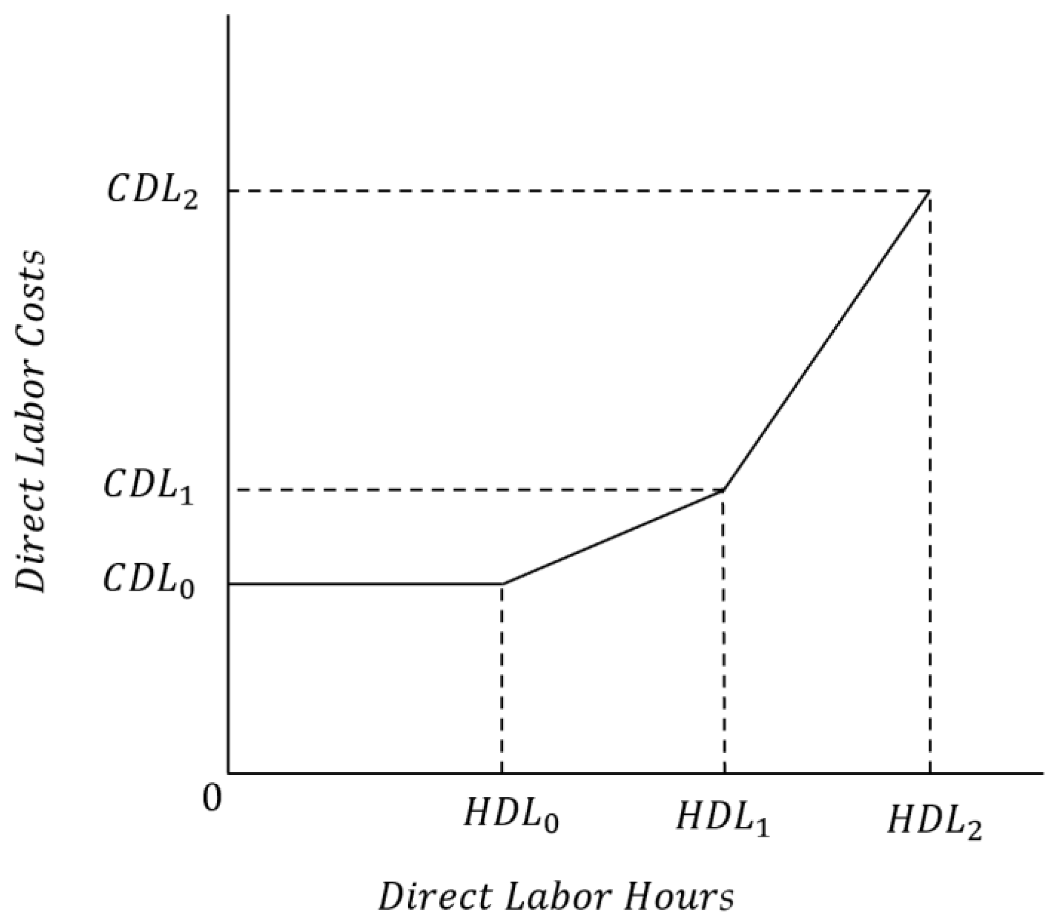
In the cement production process, direct labor, including regular and overtime hours, is a key component. This study assumes that the total direct labor cost function is a continuous piecewise linear function, as illustrated in Figure 2. If the required direct labor hours exceed regular working hours, two different wage rates are applied for the two types of labor hours. It’s assumed that the wage rates for each segment in Figure 2 are WR0, WR1, and WR2, representing different rates for varying work hour segments.
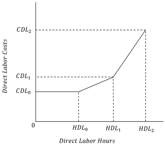
Figure 2.
Direct Labor Cost Function.
Associated constraints for the labor cost function are also defined:
Symbol Definitions:
| Quantity of the ith product in period t, (i = 1~4; t = 1~3) | |
| Non-negative variables where at most two adjacent variables are not 0, (t = 1~3) | |
| Dummy variables (0, 1), where only one can be 1 for each period (t = 1~3) | |
| Labor hours required to produce one unit of the ith product in the mth process. | |
| The total number of labor hours under normal circumstances | |
| Maximum number of labor hours falling in the first overtime segment, as shown in Figure 2 | |
| Maximum number of labor hours in the second overtime segment, as indicated in Figure 2 |
3.3.4. Batch-Level Operational Costs
It’s assumed that four operational activities in the cement production process require estimation of machine handling costs: cement grinding (m = 3) and three batching processes (m = 4, m = 5, m = 6). These costs are deducted in the profit function.
The related constraint functions are:
Symbol Definitions:
| Unit machine handling cost for the mth process | |
| Resource consumption per batch for the ith product in the mth process (i = 1~4; m = 3~6) | |
| Output per batch for the ith product in the mth process (i = 1~4; m = 3~6) | |
| Maximum available resources for the mth batch-level operation (m = 3~6) |
3.3.5. Product-Level Operational Costs
It is assumed that product-level operation costs, specifically for product batching, need to be estimated for four activities: cement grinding (m = 3) and three batching processes (m = 4, m = 5, m = 6). These product batching costs are subtracted from the profit function.
Constraint inequality includes:
Symbol Definitions:
| Unit cost of product batching for the mth process | |
| Resource consumption for the ith product in the mth process (i = 1~4; m = 3~6) | |
| Dummy variable (0, 1) for period t, determining whether the ith product is produced (i = 1~4; t = 1~3) | |
| Maximum available resources for the mth product-level operation (m = 3~6) |
3.3.6. Constraints of Machine Hours
It’s assumed that three types of automated equipment are used in the manufacturing process: raw meal grinding (m = 1), calcination (m = 2), and cement grinding (m = 3), replacing traditional manual labor to enhance efficiency.
The related constraint inequality for machine hours is:
Symbol Definitions:
| Machine hours required to complete one unit of the ith product in the mth process (m = 1~3) | |
| Upper limit of available machine hours for the mth process (m = 1~3) |
3.4. Carbon Tax Cost Function Model
3.4.1. Model 1: Continuous Incremental Progressive Tax Rate Function for Carbon Tax
This study develops a model for a continuous incremental progressive carbon tax function for the cement industry. The cost functions for multiple periods are designed to optimize profit while considering carbon tax expenses. The models are summarized as follows:
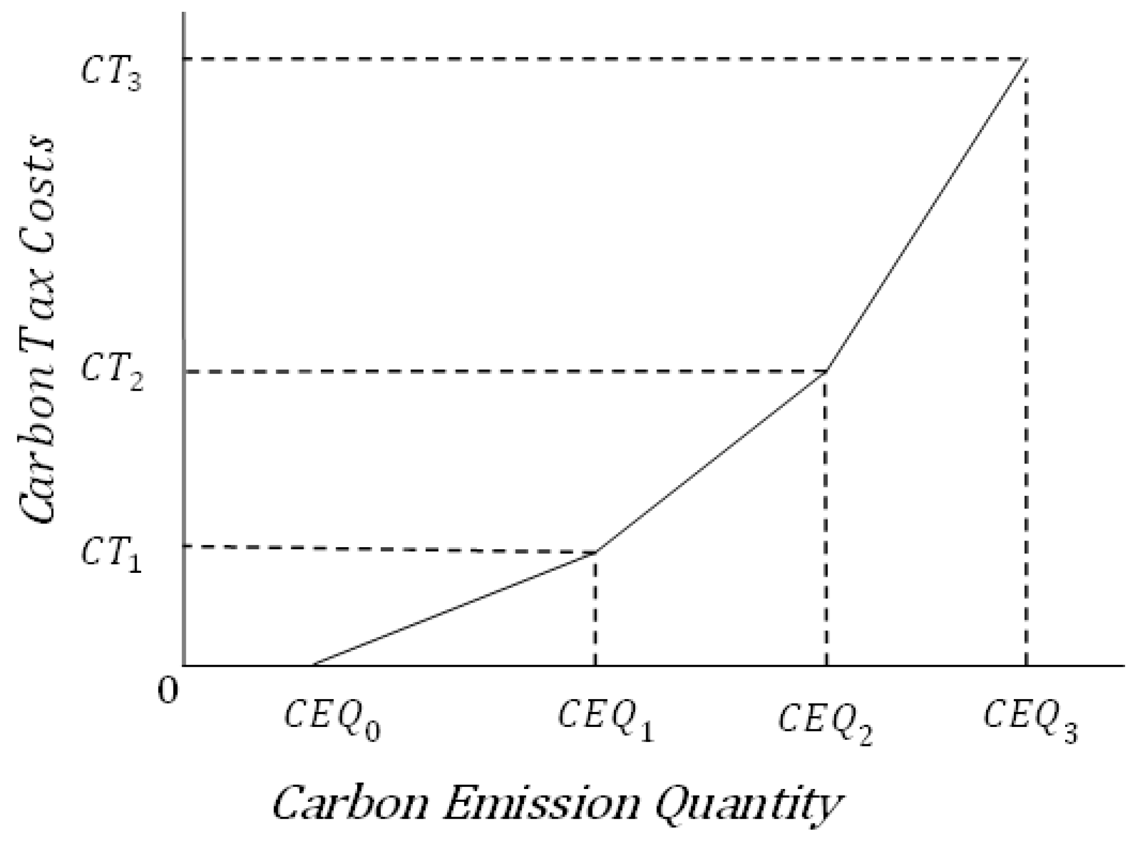
Figure 3 shows the function of carbon tax cost in the continuous incremental progressive tax rate. In Figure 3, the upper limit of carbon emission quantity in the first, second and third sections is , and , the carbon tax costs at the three points of , and are , and respectively, and the carbon tax rates are , and respectively.
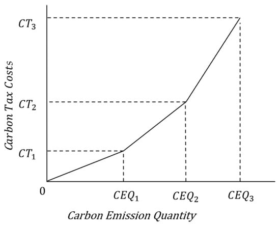
Figure 3.
Carbon Tax Costs Function with Progressive Rates.
General expression of carbon tax cost function in Figure 3 is shown as follows:
The general formula of the carbon tax cost function (15) is derived from this representation. It is a function of the company’s total carbon emissions (q) and is applied in a mathematical programming model. The model includes assumed carbon tax costs function (16), which are deducted from the company’s total profit, along with related restrictions (17)–(25).
Multi-Period Carbon Tax in Objective Function:
Related Constraints:
In Model 1, the study establishes the upper limits for carbon emissions at each stage as . The carbon emissions generated from the mth process for producing one unit of the ith product are denoted by (where m ranges from 1 to 6). The variables are non-negative, and at most two consecutive variables can be non-zero (for periods t = 1 to 3). The variables are dummies (0 or 1), with only one being 1 in any given period (t = 1 to 3). If is set to 1, the other two are zero, and in (20) and (21), would be zero, while in (18) and (19), are less than or equal to 1. In (22), the sum of equals 1. Consequently, from (17), it is determined that the total carbon emissions of the company for the first period are , and the carbon tax cost is . Alternatively, for a given period t, if = 1, then are zero by (23) and (25). It means that the carbon tax cost is in the second segment of Figure 3. On the other hand, the variables are non-negative, and at most two consecutive variables can be non-zero (for periods t = 1 to 3). If the point is in the second segment of Figure 3, then and are non-zero and their sum is 1 by (22). Thus, the corresponding carbon tax cost is by (16) and the corresponding carbon emission quantity is .
In the example, the total optimized profit across three periods (t = 1 to 3) amounts to $22,473,270,000. The profit is highest in the initial period, with subsequent periods showing a decline due to increased use of alternative materials and stricter carbon emission limits. The model also captures a decreasing trend in carbon emission ratios to over the considered timeframe.
3.4.2. Model 2: Continuous Incremental Progressive Carbon Tax Function with Tax Exemption
Model 2 of the study considers continuous incremental progressive carbon tax function with tax exemption. The carbon tax cost function of the progressive tax rate for continuous allowance increase is illustrated in Figure 4. In this figure, represents the total carbon emissions granted by the government for tax exemption, which are not subject to taxation within the carbon emission allowance. The first, second, and third interval have a capped carbon emission quantity at , and respectively. , and denote the cost of carbon tax at these respective levels while , and represent their corresponding tax rates.

Figure 4.
Continuous Incremental Progressive Carbon Tax Function with Tax Exemption.
Henceforth, we can express the carbon tax cost function in Figure 4 as function (26), which serves as a general formula encompassing continuous carbon tax costs with allowances. When calculating the company’s overall profit, it is necessary to deduct the assumed carbon tax costs specified by (27) and (28) in this model. Constraints related to the cost of carbon taxes are defined by (28)–(36).
The general formula for the carbon tax cost function is:
In a multi-period scenario, the function is defined in the objective function as:
The related constraints for the carbon tax cost function are:
Thus, it means that the mathematical fuction f(q) is represented as (27) in the objective function and the associated constraints (28)–(36). If is set to 1, then and are constrained to be zero in (31) and (32). In (29) and (30), and are limited to be less than or equal to 1. In (33), the sum of and must equal 1. Therefore, based on (28), it can be determined that the total carbon emissions of the company are less than or equal to plus , with the carbon tax cost being .
In the example, the total best profit for the enterprise across multiple periods amounts to $22,506,340,000, with the highest profit achieved in the first period. The second and third periods show lower profits due to the consideration of increased lower limits for the use of alternative materials and reduced upper limits for carbon emissions. Additionally, the carbon emission ratio demonstrates a year-over-year declining trend.
3.4.3. Model 3: Continuous Incremental Progressive Carbon Tax Function with Carbon Trading
When the government allows carbon trading, in addition to the carbon tax costs, the costs and benefits of carbon credits must also be considered. Therefore, this section extends the continuous incremental progressive carbon tax cost function of Section 3.4.1 by adding carbon trading functions to the model assumptions. This study assumes that the company uses a single carbon credit price (α) to purchase or sell carbon credits. Hence, the continuous incremental progressive carbon tax cost function, including the cost of carbon credits, is represented by (37).
The multi-period carbon tax objective function, with carbon trading, is formulated as follows:
The related constraints are as follows:
For periods t = 1 to 3, and are dummy variables, each taking a value of 0 or 1, with only one being 1 at any time. If is 1, then by (41), is 0, indicating that the company’s total carbon emissions qt fall within the range [0, ] by (39). This implies that the company doesn’t need to buy carbon credits and can even sell them, with the carbon emission costs being calculated as .
The multi-period continuous incremental progressive carbon tax function with carbon trading (Model 3) achieves an optimal profit of $22,744,860,000. By incorporating carbon credits as part of the profit function, the profits are higher compared to Model 1.
3.4.4. Model 4: Continuous Incremental Progressive Carbon Tax Objective Function (Including Tax Exemption and Carbon Credits)
This section builds upon the continuous incremental progressive carbon tax cost function from Section 3.4.1 and incorporates the tax exemption granted by the government from Section 3.4.2 as well as carbon trading from Section 3.4.3 for the model’s assumptions. The study hypothesizes that the company operates carbon trading at a single carbon credit price (α), hence the continuous incremental progressive carbon tax cost function now includes the costs of tax exemption and carbon credits as represented by (42).
For the multi-period model, the continuous incremental progressive carbon tax cost function that includes both tax exemption and carbon credits is given by:
The related constraints are as follows:
If is set to 1, then = 0 by (46). Then, by (44), the company’s total carbon emissions qt will be within the range [0, , implying the company need not buy carbon credits and may sell them instead. At this point, the carbon emission cost is given by .
3.4.5. Model 5: Discontinuous Incremental Progressive Carbon Tax Objective Function
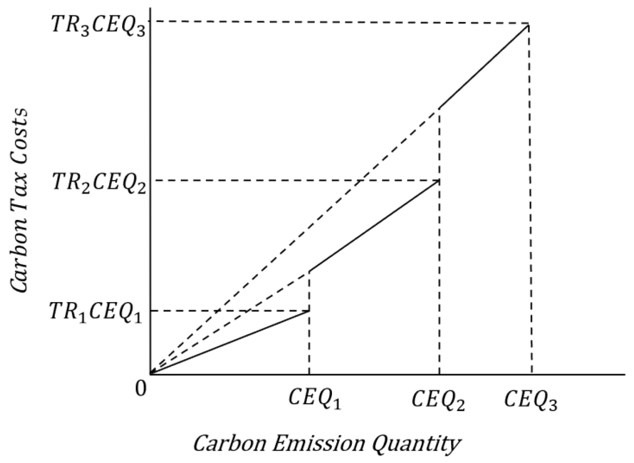
Figure 5 illustrates the carbon tax cost function for a discontinuous incremental progressive tax rate, composed of three consecutive sections. In Figure 5, the maximum carbon emission limits for the first, second, and third sections are , and , respectively. The carbon tax rates at these points are , , and , and the carbon tax costs are calculated as , , and , respectively.

Figure 5.
Discontinuous Carbon Tax Cost.
Therefore, the carbon tax cost function illustrated in Figure 5 can be represented by functions (47). This function serves as a general model for the discontinuous carbon tax cost function, which also corresponds to the company’s total carbon emissions (q) and can be represented through a mathematical programming model. Function (48) is the assumed carbon tax costs in this model and must be deducted when calculating the company’s total profit, while (49)–(54) are the constraints related to carbon tax costs.
General Expression of Carbon Tax Cost Function:
Multi-Period Discontinuous Incremental Progressive Carbon Tax Cost Function:
Related Constraints:
If is 1 in the first period, according to (53), and are 0, and thus, based on (50), the total carbon emissions for the first period fall between [0, ], and the carbon tax cost is calculated as .
3.4.6. Model 6: Discontinuous Incremental Progressive Carbon Tax Function with Tax Exemption
This section extends the discontinuous incremental progressive carbon tax function, incorporating a tax exemption as established in Model 5. The carbon tax function in Model 6 accounts for multiple periods. Figure 6 illustrates the discontinuous incremental progressive carbon tax function with tax exemption. Here, represents the total carbon emission quantity exempted from taxation by the government. The upper limits of carbon emissions for the first, second, and third segments are , and , respectively. The carbon tax costs at these points are , , and , with corresponding tax rates of 1, and .
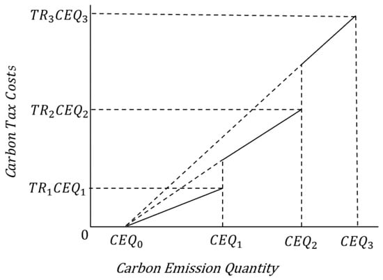
Figure 6.
Discontinuous Incremental Progressive Carbon Tax Cost with Tax Exemption.
The carbon tax cost function in Figure 6 is represented by Function (55), serving as a general model for the discontinuous carbon tax cost function with a tax exemption. This function also relates to the company’s total carbon emissions (q) and is represented through a mathematical programming model. Function (56) is the assumed carbon tax costs in this model, which must be deducted when calculating the company’s total profit. Constraints (57)–(62) are constraints related to the carbon tax costs.
General Expression of Carbon Tax Cost Function:
Multi-Period Discontinuous Incremental Progressive Carbon Tax Cost Function with Tax Exemption:
Related Constraints:
are described as dummy variables, which can only take values of 0 or 1. In this case, if is equal to 1, then according to (62), the rest of the variables must be 0. (59) suggests that this is part of a larger set of functions and conditions in the model. It implies a range or bracket of carbon emissions (, ], and the carbon tax cost for emissions within this range is given .
In the multi-period discontinuous incremental progressive carbon tax objective function—Model 6 (with tax exemption), the optimal profit is $23,958,560,000. The profit is highest in the first period and decreases in the second and third periods due to increased usage of alternative materials and lowered carbon emission limits. Additionally, the carbon emission ratio exhibits a declining trend annually.
3.4.7. Model 7: Discontinuous Incremental Progressive Carbon Tax Objective Function with Carbon Trading
With the introduction of carbon trading by the government, companies must consider the costs and benefits of carbon credits in addition to carbon tax expenses. This section continues from Model 5 (Section 3.4.5), incorporating the discontinuous incremental progressive carbon tax cost function with carbon trading functions. The study assumes that companies buy or sell carbon credits at a single price (α). Therefore, the discontinuous incremental progressive carbon tax cost function, including the cost of carbon trading, is represented by functions (64).
Multi-Period Discontinuous Incremental Progressive Carbon Tax Objective Function (Including Carbon Trading):
Relevant Constraints:
and are dummy variables (0 or 1), where only one can be 1 in a given period. If is 1, then is 0 as per (68), and the total carbon emissions fall within [0, ] as per (66). This implies the company does not need to buy carbon credits and can even sell them, making the carbon emission cost at this point .
In Model 7, which integrates carbon trading with a discontinuous incremental progressive carbon tax system. In the multi-period model, the maximum profit (MAX π) reaches $22,610,140,000. This encompasses the profits, carbon tax costs, carbon emission ratios, and material quantities for each period, with the profits being highest in the first period and gradually decreasing due to heightened use of alternative materials and stricter emission limits. The inclusion of carbon trading significantly boosts the profit compared to previous models without it.
3.4.8. Model 8: Discontinuous Incremental Progressive Carbon Tax Function with Tax Exemption and Carbon Trading
This section extends the discontinuous incremental progressive carbon tax cost function from Section 3.4.5, incorporating the tax exemption provided by the government as outlined in Section 3.4.6 and the carbon trading mechanism as detailed in Section 3.4.7. The model assumes that companies buy or sell carbon credits at a uniform price (α). Consequently, the carbon tax cost function in this model integrates the costs related to both tax exemption and carbon trading, as detailed in functions (69).
For the Multi-Period Scenario (Model 8):
Relevant Constraints:
This model defines and as dummy variables (either 0 or 1). When is 1, as per function (69), is 0. According to (73), if is 1, this indicates that the total carbon emissions of the company are within the range [0, , implying the company is not required to purchase carbon credits and may even sell them. In this case, the carbon emission costs are calculated as the sum of the costs in each segment minus the revenue from selling excess credits: .
In the multi-period scenario, the total optimal profit rises to $24,230,140,000. This increase is attributed to the model’s incorporation of tax exemptions and carbon trading, which optimizes profits across three periods. The model demonstrates the highest profitability among the discontinuous type models due to these combined factors.
4. Research Results and Analysis
4.1. Model Comparison
In this section, the analysis applies the carbon tax cost function model combined with specific model parameter assumptions. Utilizing the LINGO system, the study calculates the optimal profit, carbon tax, and ESG indicators for enterprises under various carbon tax models.
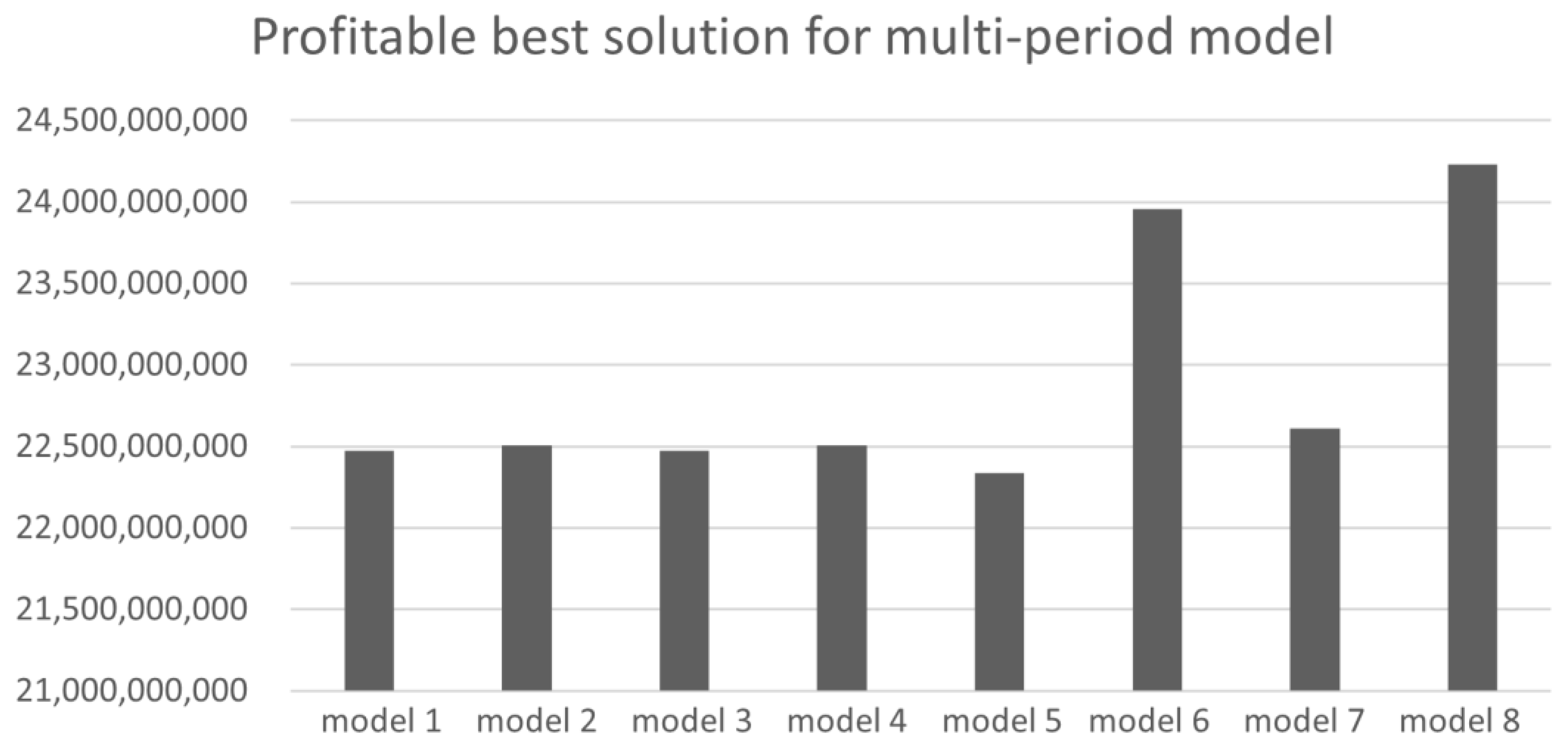
According to Figure 7, the “Discontinuous Incremental Progressive Carbon Tax Objective Function—Model 8 (Including Tax Exemption and Carbon Trading)” is identified as the optimal solution for multi-period models under the assumptions of this study. This model yields a total profit of $24,230,140,000, with annual profits of $9,447,836,000, $7,393,405,000, and $7,388,902,000 respectively. The total carbon emission cost is $3,497,046,100, with yearly costs of $902,645,400, $1,295,614,000, and $1,298,787,000.

Figure 7.
Optimal Solution for Multi-Period Models.
To meet the ESG indicators (a 11% total reduction in carbon emission ratio based on the annual carbon emission ratio limit decreases progressively, set at 0.806, 0.781, and 0.756 respectively. This indicates a yearly reduction in the carbon emission ratio per ton of clinker produced. Additionally, the usage of alternative materials () increases each year, with amounts of 1,157,457 tons, 1,309,303 tons, and 1,461,969 tons respectively.
In the discontinuous carbon tax model, Model 8 outperforms the other three models by incorporating both tax exemptions and carbon trading. With the government’s tax exemption, the first tier of carbon emissions allows for more emissions compared to Model 5, which does not include a tax exemption. This means that the same cost permits more carbon emissions. Furthermore, Model 8 includes carbon trading, allowing the sale of unused carbon credits or the purchase of additional credits to increase emissions. Thus, Model 8 achieves the highest profit within this category of carbon tax models.
In the multi-period model’s carbon emission cost chart, it’s observed that Models 6 and 8 have significantly lower carbon emission costs compared to other models, primarily due to the incorporation of tax exemptions. When tax exemptions are factored into these models, carbon emissions within the government-granted tax-free emission total are not taxed. This setup means that models considering tax exemptions have relatively lower carbon emission costs for the same amount of emissions compared to other models. In other words, at the same carbon emission cost, these models can afford more carbon emissions. This allowance provides businesses the flexibility to consider increasing production to boost revenue. Additionally, if the carbon tax cost is lower than the carbon credit cost (α), these credits can be sold to other enterprises in need, increasing profit from carbon trading.
While Model 8 is identified as the optimal solution for multi-period models under the study’s assumptions, it does not have the lowest carbon emission costs. Model 6 holds this distinction, mainly because Model 8, unlike Model 6, includes carbon trading as a cost consideration. If the carbon tax cost is lower than the carbon credit cost (α), Model 8 can sell its carbon credits to other enterprises, thus boosting its profitability. Therefore, although Model 8 does not have the lowest carbon emission cost, its inclusion of carbon trading makes it the best solution among the multi-period models.
4.2. Sensitivity Analysis
This study conducts sensitivity analyses to assess the future impact of carbon tax and carbon credit policies. By altering the unit cost of carbon credits and taxes between −20% and +20% (in 10% increments) while keeping other parameters constant, the study generates additional data for multi-period scenarios. These analyses aim to understand how changes in carbon-related costs affect profitability, offering insights into the financial implications of evolving environmental regulations and market conditions.
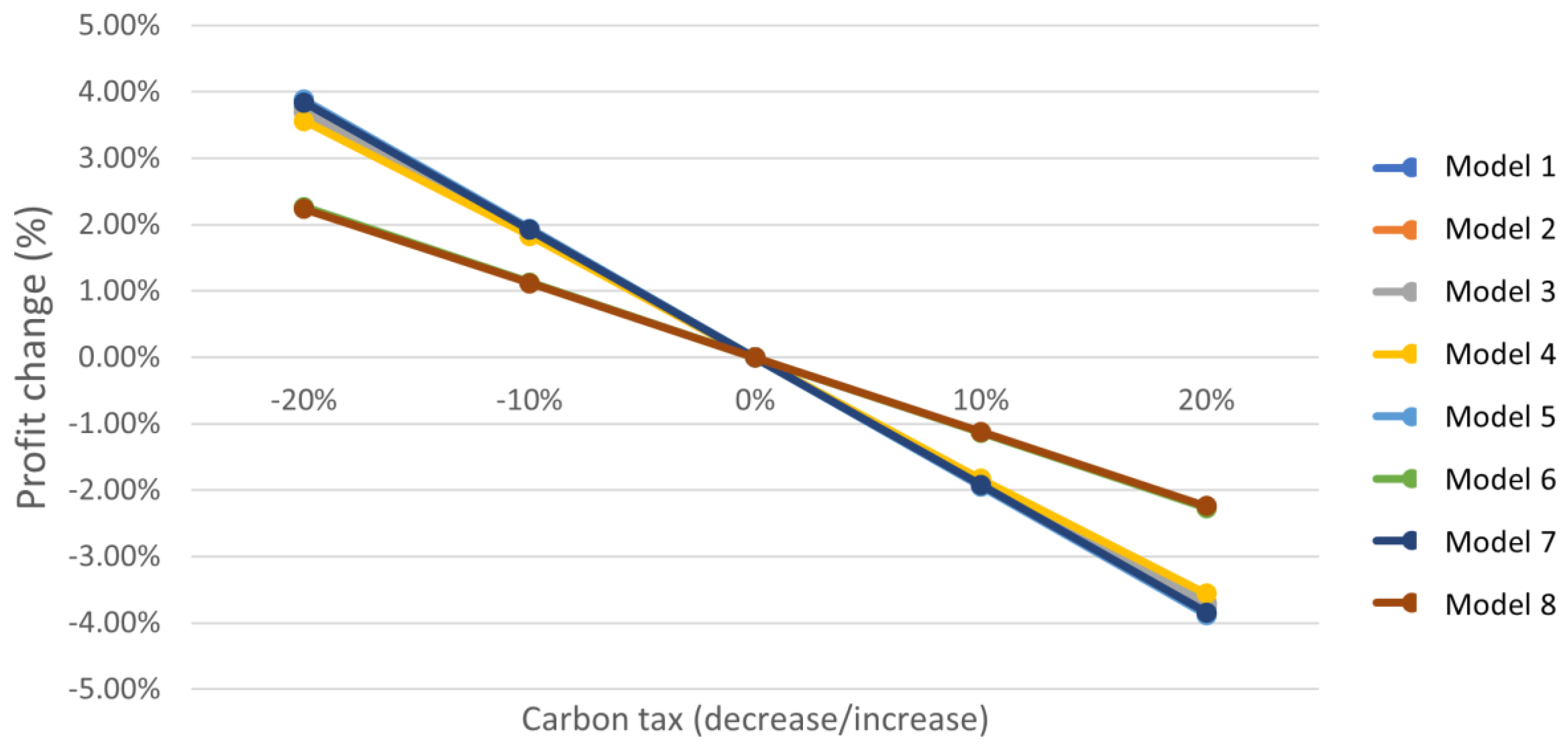
In the multi-period model of sensitivity analysis, the parameters other than the unit cost of carbon tax remain unchanged. The carbon tax cost is adjusted from −20% to +20%, in 10% increments, to generate four different data outcomes. This analysis aims to explore the impact of carbon tax cost variations on profitability. The results, as depicted in Figure 8, show a negative correlation between the carbon tax unit price and profit. Specifically, an increase in the carbon tax unit price leads to a rise in carbon tax costs, resulting in a decrease in profitability.
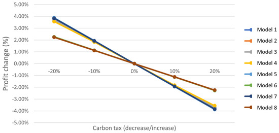
Figure 8.
Comparison of Sensitivity Analysis in Multi-period Model.
Furthermore, Figure 8 reveals that the impact of changes in carbon tax unit costs is relatively lower for Models 6 and 8. This is attributed to the fact that both models employ a discontinuous incremental progressive tax rate and include tax exemptions in their cost calculations. Under this tax structure, both models fall within the first bracket of the carbon tax, where the unit price is fixed. Additionally, Model 8, unlike Model 6, incorporates carbon trading as a cost consideration. This results in a lower proportion of carbon tax cost in the total revenue for Model 8. Therefore, fluctuations in carbon tax prices have a less significant impact on profitability for Model 8 compared to Model 6.
5. Discussion
LINGO 20 [43] is adopted in this study to solve the optimization models with carbon tax and emissions trading considerations, owing to its computational efficiency, flexibility in handling complex constraints and large-scale models, and integration with Excel for results validation. The customized modeling languages in LINGO are particularly applicable for linear, nonlinear, integer programs, fitting the characteristics of the cement production model proposed. It also allows incorporating logical conditions and branch-and-bound algorithms to facilitate the modeling of tiered carbon tax rates and trading decisions. By linking the optimization solutions with Excel analysis, the model results can compare profits, carbon emissions, and other indices under varying policy scenarios to provide scenario-based decision support for enterprises and policymakers, balancing between environmental and economic interests.
This study reveals that the discontinuous progressive carbon tax structure integrated with carbon trading (Model 8) leads to optimal profitability performance. This finding differs from several existing studies suggesting continuous incremental tax rates as the predominant option. The divergence could stem from this study’s simultaneous consideration of both differential tax models and emissions trading schemes. Specifically, the initial milder tax burden during the introductory phases of a graduated carbon tax system allows more flexibility that, when combined with the carbon market mechanisms, could offer a balanced approach accommodating environmental targets and business interests. Hence, the research results underline the importance of evaluating integrative tax and trading policy scenarios to fully assess and leverage potential synergistic effects. As a pioneering empirical attempt at such holistic examination tailored to the cement industry, this study paves the way for further validation through expanded real-world case studies across different sectors. Related future research could also explore optimal transitional paths for emerging economies applying differentiated policy instruments judiciously to progress towards carbon neutrality.
6. Conclusions and Recommendations
Analysis of Different Carbon Tax Models: In the investigation of various carbon tax structures, Models 5 and 6, which utilize a discontinuous progressive tax framework, show superior profitability in comparison to Models 1 and 2 that implement a continuous progressive tax approach. These findings suggest that for businesses, the deployment of discontinuous progressive tax rates by governments can lead to a lessened carbon tax burden. Moreover, for governments, the adoption of discontinuous tax rates initially offers a milder impact on enterprises, thus aiding their transition towards comprehensive carbon tax systems. Additionally, the study explores the integration of carbon trading into these models. The introduction of carbon trading has been found to enable businesses to attain higher profits within established carbon emission limits. Notably, Model 8, incorporating carbon trading, stands out as the optimal choice, highlighting that incorporating carbon trading mechanisms does not adversely impact the expected tax revenues for governments.
This study provides several policy implications. The discontinuous carbon tax structure could serve as a transition mechanism for governments, balancing the goals of emission reduction and business interests. The gradual rate ramp-up grants company time to adapt while maintaining revenues. Moreover, incorporating carbon trading schemes further eases tax burdens. With proper design integration, environmental targets could align with economic sustainability
Striking a balance between environmental conservation and business growth is crucial, particularly in the context of carbon tax implications on companies and consumers. Increased carbon taxes could result in higher product prices from companies, potentially impacting consumer expenses and aggravating inflation. Hence, it’s essential to identify strategies that align ecological preservation with commercial development. In the cement industry, embracing sustainable practices is key. By refining production processes and utilizing alternative materials for industrial waste management, companies can decrease expenses and boost efficiency. These measures are pivotal in reducing the environmental impact of cement manufacturing and promoting effective resource utilization.
In crafting carbon tax and trading policies, it is crucial for policymakers to carefully consider their impact on businesses and the broader economy, fostering an environment where companies are motivated to pursue eco-friendly alternatives and innovative solutions for improved environmental outcomes. Concurrently, enterprises are encouraged to proactively seek out and implement green alternatives and advanced technologies to effectively address the challenges posed by these policies. By investing in sustainable production methods, businesses can enhance their competitiveness and secure long-term benefits. This holistic approach not only promotes environmental protection but also ensures the economic sustainability of businesses, paving the way for greater opportunities in green development and aligning economic objectives with environmental stewardship.
Future Research Directions: The model established in this paper only considers the case of a single company and does not reflect the impact of the overall carbon market dynamics on credit pricing. Further models could be developed by incorporating an assessment of the aggregate supply and demand and trading activities in the carbon market, linking the carbon tax cost function to market prices. This would further enhance the adaptability of model outcomes.
It should be noted that this study only focuses on the cement industry, and the uniqueness of the industry may limit the generalizability of the research findings to other industries. To broaden the impact, follow-up studies could consider applying similar methods to analyze other high carbon-emitting industries, or conduct horizontal comparisons to examine the differences between industries. This would help gain more comprehensive insights.
Author Contributions
Conceptualization, W.-H.T. and W.-H.L.; methodology, W.-H.L.; investigation, W.-H.L.; writing—original draft, W.-H.L.; writing—review and editing, W.-H.T.; supervision, W.-H.T.; funding acquisition, W.-H.T. All authors have read and agreed to the published version of the manuscript.
Funding
The authors would like to thank the National Science and Technology Council of Taiwan for the financial support of this research under Grant No. MOST111-2410-H-008-021 and MOST112-2410-H-008-061.
Institutional Review Board Statement
Not applicable.
Informed Consent Statement
Not applicable.
Data Availability Statement
The author confirms that the data supporting the findings of this study are available within the article.
Conflicts of Interest
The authors declare no conflict of interest.
References
- Wolniak, R.; Wyszomirski, A.; Olkiewicz, M.; Olkiewicz, A. Environmental corporate social responsibility activities in heating industry—Case study. Energies 2021, 14, 1930. [Google Scholar] [CrossRef]
- Yoon, B.; Lee, J.H.; Byun, R. Does ESG performance enhance firm value? Evidence from Korea. Sustainability 2018, 10, 3635. [Google Scholar] [CrossRef]
- Dinga, C.D.; Wen, Z. China’s green deal: Can China’s cement industry achieve carbon neutral emissions by 2060? Renew. Sustain. Energy Rev. 2022, 155, 111931. [Google Scholar] [CrossRef]
- Tesema, G.; Worrell, E. Energy efficiency improvement potentials for the cement industry in Ethiopia. Energy 2015, 93, 2042–2052. [Google Scholar] [CrossRef]
- Wang, N. Environmental Production: Use of Waste Materials in Cement Kilns in China. Master’s Thesis, Høgskolen i Telemark, Porsgrunn, Norway, 2008. [Google Scholar]
- Zhu, Q. CO2 Abatement in the Cement Industry; IEA Clean Coal Centre: 2011. Available online: https://usea.org/sites/default/files/062011_CO2%20abatement%20in%20the%20cement_ccc184.pdf (accessed on 26 February 2024).
- Watson, J.G.; Chow, J.C. Protocol for Applying and Validating Receptor Model Source Apportionment in PMEH Study Areas; Desert Research Institute: Washington, DC, USA, 2018. [Google Scholar]
- Cai, W.; Wang, C.; Chen, J.; Wang, K.; Zhang, Y.; Lu, X. Comparison of CO2 emission scenarios and mitigation opportunities in China’s five sectors in 2020. Energy Policy 2008, 36, 1181–1194. [Google Scholar] [CrossRef]
- Talaei, A.; Pier, D.; Iyer, A.V.; Ahiduzzaman, M.; Kumar, A. Assessment of long-term energy efficiency improvement and greenhouse gas emissions mitigation options for the cement industry. Energy 2019, 170, 1051–1066. [Google Scholar] [CrossRef]
- Yang, L.; Xia, H.; Zhang, X.; Yuan, S. What matters for carbon emissions in regional sectors? A China study of extended STIRPAT model. J. Clean. Prod. 2018, 180, 595–602. [Google Scholar] [CrossRef]
- Dong, C.; Dong, X.; Jiang, Q.; Dong, K.; Liu, G. What is the probability of achieving the carbon dioxide emission targets of the Paris Agreement? Evidence from the top ten emitters. Sci. Total. Environ. 2018, 622–623, 1294–1303. [Google Scholar] [CrossRef]
- Li, W.; Gao, S. Prospective on energy related carbon emissions peak integrating optimized intelligent algorithm with dry process technique application for China’s cement industry. Energy 2018, 165, 33–54. [Google Scholar] [CrossRef]
- Shen, W.; Cao, L.; Li, Q.; Zhang, W.; Wang, G.; Li, C. Quantifying CO2 emissions from China’s cement industry. Renew. Sustain. Energy Rev. 2015, 50, 1004–1012. [Google Scholar] [CrossRef]
- Obrist, M.D.; Kannan, R.; Schmidt, T.J.; Kober, T. Decarbonization pathways of the Swiss cement industry towards net zero emissions. J. Clean. Prod. 2021, 288, 125413. [Google Scholar] [CrossRef]
- Fang, D.; Zhang, X.; Yu, Q.; Jin, T.C.; Tian, L. A novel method for carbon dioxide emission forecasting based on improved Gaussian processes regression. J. Clean. Prod. 2018, 173, 143–150. [Google Scholar] [CrossRef]
- Junianto, I.; Sunardi; Sumiarsa, D. The Possibility of Achieving Zero CO2 Emission in the Indonesian Cement Industry by 2050: A Stakeholder System Dynamic Perspective. Sustainability 2023, 15, 6085. [Google Scholar] [CrossRef]
- Ofosu-Adarkwa, J.; Xie, N.; Javed, S.A. Forecasting CO2 emissions of China’s cement industry using a hybrid Verhulst-GM(1,N) model and emissions’ technical conversion. Renew. Sustain. Energy Rev. 2020, 130, 109945. [Google Scholar] [CrossRef]
- Hsieh, C.-L.; Tsai, W.-H. Sustainable Decision Model for Circular Economy towards Net Zero Emissions under Industry 4.0. Processes 2023, 11, 3412. [Google Scholar] [CrossRef]
- Tsai, W.-H.; Lu, Y.-H.; Hsieh, C.-L. Comparison of production decision-making models under carbon tax and carbon rights trading. J. Clean. Prod. 2022, 379, 134462. [Google Scholar] [CrossRef]
- Zaklan, A. Coase and Cap-and-trade: Evidence on the independence property from the European carbon market. Am. Econ. J. Econ. Policy 2023, 15, 526–558. [Google Scholar] [CrossRef]
- Peng, Z.; Lu, W.; Webster, C. If invisible carbon waste can be traded, why not visible construction waste? Establishing the construction waste trading ‘missing market’. Resour. Conserv. Recycl. 2022, 187, 106607. [Google Scholar] [CrossRef]
- Arvidsson, S.; Dumay, J. Corporate ESG reporting quantity, quality and performance: Where to now for environmental policy and practice? Bus. Strat. Environ. 2022, 31, 1091–1110. [Google Scholar] [CrossRef]
- Clément, A.; Robinot, É.; Trespeuch, L. Improving ESG scores with sustainability concepts. Sustainability 2022, 14, 13154. [Google Scholar] [CrossRef]
- Taiwan Cement Corporation. Taiwan Cement Sustainability Report. 2022. Available online: https://www.taiwancement.com/tw/esgIndex.html (accessed on 3 May 2022).
- Turney, P.B.B. Common Cents: The ABC Performance Breakthrough: How to Succeed with Activity-Based Costing; McGraw-Hill: New York, NY, USA, 2005. [Google Scholar]
- Tsai, W.H.; Lin, T.W.; Chou, W.C. Integrating Activity-Based Costing and Environmental Cost Accounting Systems: A Case Study. Int. J. Bus. Syst. Res. 2010, 4, 186. [Google Scholar] [CrossRef]
- Jasch, C. The use of Environmental Management Accounting (EMA) for identifying environmental costs. J. Clean. Prod. 2003, 11, 667–676. [Google Scholar] [CrossRef]
- Bento, N.; Gianfrate, G.; Aldy, J.E. national climate policies and corporate internal carbon pricing. Energy J. 2021, 42, 89–100. [Google Scholar] [CrossRef]
- Sánchez-Rebull, M.-V.; Niñerola, A.; Hernández-Lara, A.-B. After 30 Years, What Has Happened to Activity-Based Costing? A Systematic Literature Review. SAGE Open 2023, 13. [Google Scholar] [CrossRef]
- Al-Hashimi, A.M.; Al-Ghazal HA, A.-S. Towards corporate sustainability: Cost-benefit considerations of quantitative methods (multiple regression model) versus activity-based methods for determining indirect costs—An applied study in KDD industrial company. AIP Conf. Proc. 2023, 2776, 100005. [Google Scholar] [CrossRef]
- Al-Sayed, M.; Dugdale, D. Activity-based innovations in the UK manufacturing sector: Extent, adoption process patterns and contingency factors. Br. Account. Rev. 2016, 48, 38–58. [Google Scholar] [CrossRef]
- Cannavacciuolo, L.; Illario, M.; Ippolito, A.; Ponsiglione, C. An activity-based costing approach for detecting inefficiencies of healthcare processes. Bus. Process. Manag. J. 2015, 21, 55–79. [Google Scholar] [CrossRef]
- Demdoum, Z.; Meraghni, O.; Bekkouche, L. The Application of Green Accounting According to Activity-Based Costing for an Orientation Towards a Green Economy: Field Study. Int. J. Digit. Strat. Gov. Bus. Transform. 2021, 11, 1–15. [Google Scholar] [CrossRef]
- French, K.E.; Guzman, A.B.; Rubio, A.C.; Frenzel, J.C.; Feeley, T.W. Value based care and bundled payments: Anesthesia care costs for outpatient oncology surgery using time-driven activity-based costing. In Healthcare; Elsevier: Amsterdam, The Netherlands, 2016; Volume 4, pp. 173–180. [Google Scholar]
- Quesado, P.; Silva, R. Activity-Based Costing (ABC) and Its Implication for Open Innovation. J. Open Innov. Technol. Mark. Complex. 2021, 7, 41. [Google Scholar] [CrossRef]
- AL Mashkoor, I.A.S.; Ali, J.H.; Al-Kanani, M.M. The Role of Green Activity-Based Costing in Achieving Sustainability Development: Evidence From Iraq. Int. J. Prof. Bus. Rev. 2023, 8, e01276. [Google Scholar] [CrossRef]
- Tsai, W.-H.; Chang, J.-C.; Hsieh, C.-L.; Tsaur, T.-S.; Wang, C.-W. Sustainability concept in decision-making: Carbon tax consideration for joint product mix decision. Sustainability 2016, 8, 1232. [Google Scholar] [CrossRef]
- Goldratt, E.M.; Cox, J. The Goal: A Process of Ongoing Improvement; North River Press: Great Barrington, MA, USA, 1992. [Google Scholar]
- Burange, L.G.; Yamini, S. Performance of the Indian cement industry: The competitive landscape. Artha Vijnana 2009, 51, 209. [Google Scholar] [CrossRef]
- Demirel, E.; Eskin, İ. Relation between environmental impact and financial structure of cement industry. Int. J. Energy Econ. Policy 2017, 7, 129–134. [Google Scholar]
- Panizzolo, R. Theory of constraints (TOC) production and manufacturing performance. Int. J. Ind. Eng. Manag. 2016, 7, 15–23. [Google Scholar] [CrossRef]
- Mabin, V.J.; Balderstone, S.J. The performance of the theory of constraints methodology: Analysis and discussion of successful TOC applications. Int. J. Oper. Prod. Manag. 2003, 23, 568–595. [Google Scholar] [CrossRef]
- LINGO 20: Mathematical Programming Software; Optimization Modeling Software for Linear, Nonlinear, and Integer Programming. Available online: https://www.lindo.com/index.php/ls-downloads/try-lingo (accessed on 26 February 2024).


Disclaimer/Publisher’s Note: The statements, opinions and data contained in all publications are solely those of the individual author(s) and contributor(s) and not of MDPI and/or the editor(s). MDPI and/or the editor(s) disclaim responsibility for any injury to people or property resulting from any ideas, methods, instructions or products referred to in the content. |
© 2024 by the authors. Licensee MDPI, Basel, Switzerland. This article is an open access article distributed under the terms and conditions of the Creative Commons Attribution (CC BY) license (https://creativecommons.org/licenses/by/4.0/).