Sensitivity-Based Permutation to Balance Geometric Inaccuracies in Modular Structures

Abstract

In modular structures, inaccuracies of the modules superimpose over the entire structure. Depending on the placement of the modules, these inaccuracies have (different) effects on stresses and total deformations. Especially for structures with many individual modules, it is favorable to place them according to their influence. To cover structural diversity, column-, beam-, and wall-like modular structures made from plane modules are investigated. In numerical simulation, geometric inaccuracies are applied via an equivalent temperature approach, which allows almost arbitrary nodal deviations of the modules. With the elementary effects method, the sensitivities of the modules’ inaccuracies regarding their structural impact can be determined with minimal computational effort. On a predefined control node, the overall structural inaccuracies are examined in a simplified manner. Column-like structures experience higher deformations due to inclination than beam-like or wall-like structures. For column-like, the bottommost modules are decisive for the overall inaccuracy, as they contribute significantly to the inclination. By contrast, modules at the supports are identified as particularly sensitive for beam- and wall-like structures. Controlling module placement towards their mean absolute influence, the deformation at the control node is mathematically reduced by at least 43% compared to random placement. Thereby, even modules that do not comply with tolerance requirements for structural components can be used in areas of low influence for a sustainable and low-waste design.

1. Introduction

Modular structures are built up from (precast concrete) components. These offer the advantage that they can be prefabricated in a quality-assured, automated manner [1]. Thus, construction on site is limited to the mere assembly of the modules, which considerably accelerates the building process. This is common practice in steel construction. Components are delivered and connected in situ by simple screwing while tolerances are compensated for, e.g., by hole clearance of few millimeters. Prefabricated concrete components, however, exhibit tolerances in the range of centimeters, so that joining usually means subsequent casting [2]. Although even high tolerances can be compensated for, it again results in hardening times due to the additional casting on-site. This can delay subsequent work and thus the progress of construction. Alternative joining methods are, e.g., (pre-stressed) dry joints [3,4], shear [5] or tension joints [6]. An overview of different approaches (for modular structures) is given in [7,8,9]. Yet, if the joints are not tolerance-compensating, the tolerance requirements on the individual components increase simultaneously, since inaccuracies of the components or connections sum up over the whole structure [2].

Modular construction [10] is most effective when the same element is mass-produced in automated fashion [1]. Therefore, structures are segmented into a large number of equal (or similar) components that form construction kits [11,12,13,14]. The components of these kits can even be structurally optimized for low-weight, sustainable and resource-efficient design [15,16,17]. Additionally, the production can be accelerated by non-standard heat treatment of the concrete elements [18]. The assembly is achieved by means of simple screwing or dry joints [19]. Thereby, high tolerance requirements, which come with higher production costs, emerge [20]. In addition, proper assembly in situ should be ensured to avoid delays due to reworking or replacement of modules. On the one hand, this should be ensured by high standards of quality assurance in production [21,22], e.g., by suited measurement techniques [23,24,25] of the components. On the other hand, if the tolerance requirements of the components are too high, tolerance-compensating placement strategies can be exploited.

Classical approaches to determine tolerance requirements often use tolerance chains that are mainly additive models and restricted to 1D (or 2D directed) problems [26]. Advanced approaches, e.g., using Monte Carlo simulation [27,28], can be used to control the fabrication process but are also limited to the prediction of joint tolerances, however, in a more accurate way. But, all of these tolerance analysis methods do not incorporate compensation of tolerances in assembly. So, appropriate tolerance management [29] can mitigate tolerance requirements by an improved analysis but is not able to outbalance module tolerances within a structure. However, in mechanical engineering, for example, pairing strategies have become established in which “too long” components are paired with equally “too short” components in order to minimize scrap [30]. Aligning and balancing deviations of the modules with the help of optimization-based permutation strategies, such as meta-heuristics [31,32,33], can be used for compensation, but these are usually computationally intensive [34]. In consequence, a direct balancing of module inaccuracies is too expensive for modular structures consisting of a multitude of modules. However, sensitivity analysis, in particular by screening methods [35,36,37] as qualitative methods, has been proven to enable distinguishing relevant from non-relevant parameters with reduced computational effort. Here, those positions within a modular structure that are most sensitive regarding the global deformation are identified first. Then the modules, which possess certain geometric inaccuracies, can be permuted depending on their influence on the superimposed deformation of the structure to outbalance inaccuracies afterwards.

The general procedure of the sensitivity-based permutation method, derived in this paper, is visualized in Figure 1. Geometric inaccuracies of concrete modules are transferred into equivalent temperature constraints within a finite element (FE) environment. They serve as initial deformations within modular structures. For convenience, plane structures are investigated here, which are modeled as column-, beam-, or wall-like structures depending on the number of modules in their spatial directions. Then, the modules that have a significant influence on the superimposed structural deformations—for an examined control node—are determined by means of sensitivity analysis. Depending on the sensitivities, placement is permuted so that more accurate modules are placed in the influential regions to minimize structural inaccuracy. The sensitivity-based permutation is then evaluated by means of Monte Carlo analysis of the structural deformation. In particular, the efficient Latin Hypercube Sampling (LHS) technique is used to sample the geometric inaccuracies of the modules. The evaluation bases on statistical analysis of the resulting structural deformations.

2. Materials and Methods

2.1. Tolerances of Concrete Modules

Concrete modules possess geometric deviations ∆l, which arise from different sources and are usually superimposed. These can be divided into induced, i.e., initial deviations from the production process, and inherent deviations, i.e., load- or material-related, but also transient inaccuracies [38]. The former largely depend on the type of formwork used, the care taken, and the measurement methods chosen, while the latter capture, for example, shrinkage [18] and creep deformations [39].

Geometric deviations are usually specified as tolerances t. These tolerances define limit values that a component exhibits with a certain probability P ϵ [0; 1] of an underlying Gaussian distribution. Precast concrete components usually have relatively low accuracy or high scatter, respectively. Therefore, it is assumed that 95.45% of the expected deviations fall within tolerance limits, which corresponds to two times the standard deviation σ [38]. The limits of t are thus associated with the probabilities P = [0.02275; 0.97725]. By comparison, in mechanical engineering, the so-called 6σ-principle was established to meet high fitting requirements [40]. Its fulfillment means that only 2 out of a billion components do not comply with the tolerances. Yet, these requirements seem hardly transferable to concrete components.

In this work, the geometric deviations ∆l are randomly generated by inverse transformation through a Gaussian distribution, whereby the limits correspond to twice the standard deviation for concrete components as outlined above. The mean value is chosen to be 0, so that no systematic errors are considered for the initial deviations of a module.

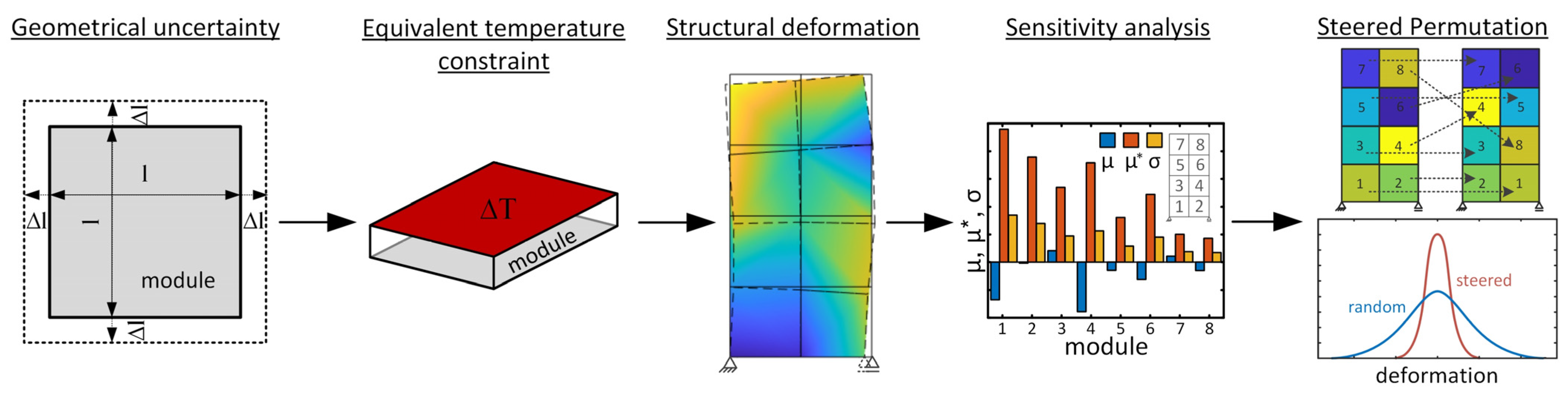
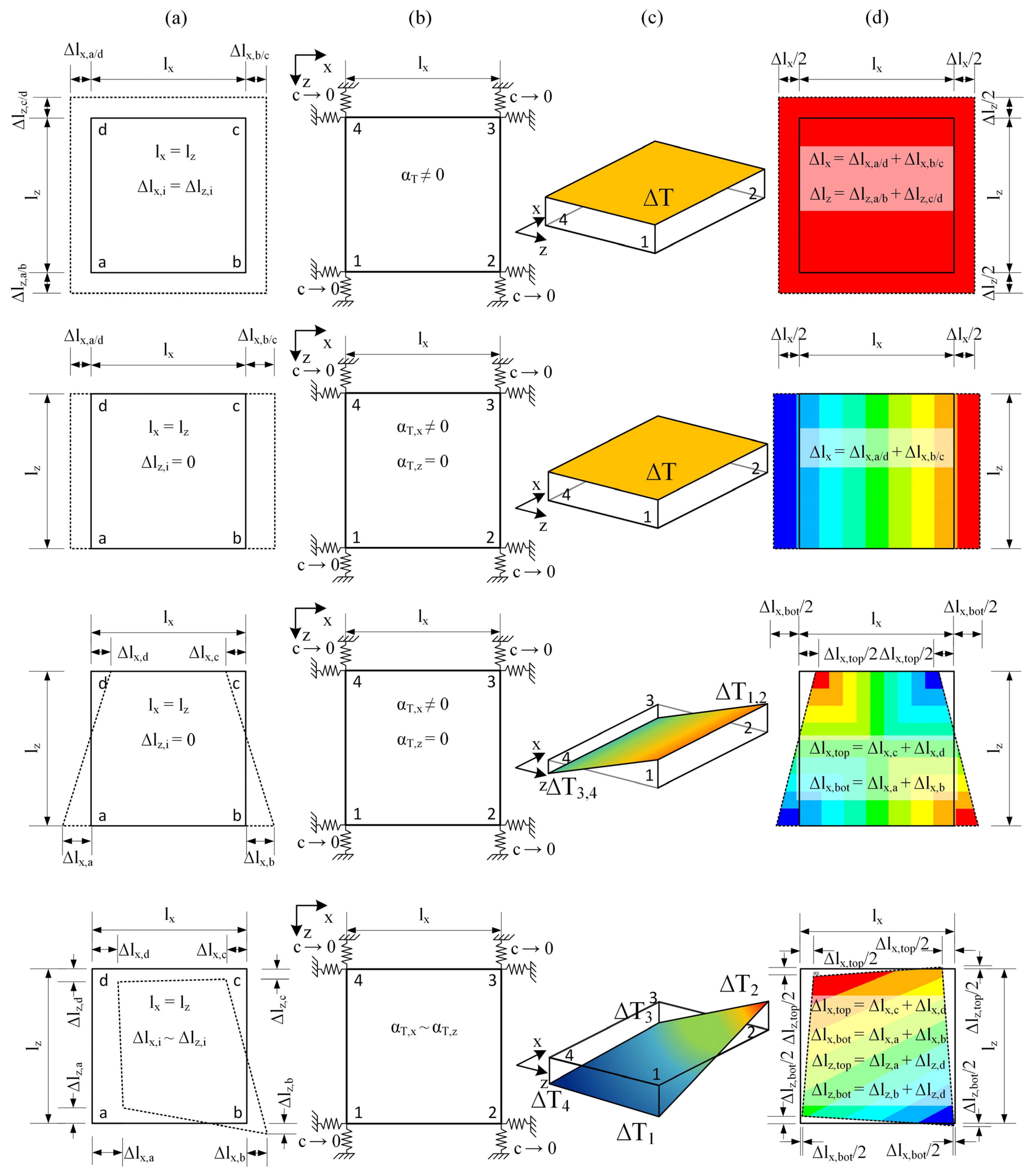
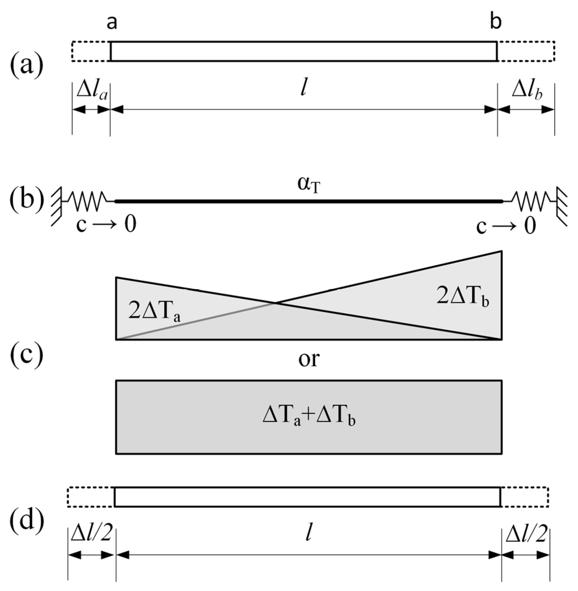
2.2. Modelling Geometric Deviations Using Temperature Constraints

If a solid component is subjected to temperature variation ∆T, its geometric dimensions change depending on the thermal expansion coefficient α_T. For the one-dimensional case, the lengthening ∆l related to the total length l of the component is the thermal strain ${\epsilon }_T$ and calculated as follows:

$$\frac{\mathsf{\Delta }l}{l}={\alpha }_{\mathrm{T}}\mathsf{\Delta }T={\epsilon }_T$$

(1)

Vice versa, the temperature variation ∆T can be determined for which a certain initial deviation ∆l is caused. Thus, geometric deviations can be introduced into a module via equivalent temperature constraints.

The general procedure is shown in Figure 2 on a truss-like element. In (a) the element exhibits nominal length l and initial deviations of ∆l_a and ∆l_b at its nodes a and b. The member is modeled by means of a 1D structural FE with linear shape functions and a thermal expansion coefficient α_T. Support is provided by springs at the nodes a and b in order to avoid kinematics, but with very low stiffness (c → 0) to permit deformation due to temperature constraints (b). For each node, ∆T_a or ∆T_b is determined from Equation (1).

However, the appropriate nodal deviation always bases on the total deformation of the module, i.e., resulting from a constant temperature constraint over the length of the module. If a specific deviation at one node should be directly applied to the module, the respective nodal temperature must be doubled (c). This is due to the always linear course of the temperature for isotropic elements. In general, different deviations for both nodes can separately be considered and superposed. Then a constant temperature constraint over the module, resulting from the sum of ∆T_a and ∆T_b, is prescribed ((c), bottom). The area under the constant temperature curve over the length l complies to the sum of the two triangular distributions ((c), top). The temperature constraint in turn results in a total geometric deviation ∆l, which is divided equally on the two nodes of the module (d). And ∆l corresponds to the sum of ∆l_a and ∆l_b. Geometric inaccuracies can thus not be implemented as direct deformations at the nodes, but as absolute deformations for the whole module.

It should be noted that in principle, the local nodal deviations could also be implemented via temperature constraints. Fixed supports at the position where the mean deformation occurs—which is initially unknown and would have to be derived additionally—must then be implemented. But this greatly complicates the modeling. Moreover, the superposition of the inaccuracies of several modules in structures is then no longer possible.

The transfer of the proposed approach to plane elements (2D) is straightforward. Figure 3 shows the plane case for given but different initial deviations and the associated boundary conditions of the FE model. It consists of a quadratic module with the outer dimensions l_x = l_z (a), which exhibits the initial deviations ∆l_x and ∆l_z at the nodes a, b, c, and d, respectively. The module is designed as a plane finite element with linear shape functions, whose thermal expansion coefficients α_T,x and α_T,z can be defined separately for the spatial directions. Support is provided through directional springs at all nodes, which again have very low stiffness (c → 0) to permit deformations (b). The geometric deviations at the nodes are converted into temperature constraints (c) according to Equation (1). Assuming again a linear course of the temperature distribution, the equivalent ∆T_i per node i corresponds to twice the equivalent temperature. The deformations from finite element analysis (FEA) are shown in (d). It must be noted that the deviations per node are derived separately for the spatial x- and z-directions according to Equation (1). Since for both directions, the same ∆T is used, differences between the deviations are incorporated through the ratio of the thermal expansion coefficients α_T,x and α_T,z.

Four characteristic sets of deformations are obtained from prescribed initial geometric deviations at the nodes shown in Figure 3, from top to bottom:

• Constant plane deformation in both directions (${\alpha }_{\mathrm{T},\mathrm{x}}~{\alpha }_{\mathrm{T},\mathrm{z}}\ne 0,$ ∆T = const.);
• Constant plane deformation in one direction (${\alpha }_{\mathrm{T},\mathrm{x}}\vee {\alpha }_{\mathrm{T},\mathrm{z}}=0,$ ∆T = const.);
• Linear variable deformation over the height (${\alpha }_{\mathrm{T},\mathrm{x}}\ne 0, {\alpha }_{\mathrm{T},\mathrm{z}}=0,$ ∆T₁ = ∆T_2, ∆T₃ = ∆T₄);
• (Almost) arbitrary deformation at the nodes (${\alpha }_{\mathrm{T},\mathrm{x}}~{\alpha }_{\mathrm{T},\mathrm{z}},$ ∆T = var.).

Constant deformations are achieved through a constant ∆T. If deformation should be one directional, α_T must be set to 0 in the other direction. Different deformations for the same dimensions in x- and z-direction can be achieved, fixing the ratio of the deviations as follows:

$${\alpha }_{\mathrm{T},\mathrm{z}}={\alpha }_{\mathrm{T},\mathrm{x}}\left(\frac{\mathsf{\Delta }{l}_{\mathrm{z}}}{\mathsf{\Delta }{l}_{\mathrm{x}}}\right)$$

(2)

A similar approach is possible if the element is not quadratic, but the same deviations are to be applied in both directions (∆l_x = ∆l_z). Through Equation (1), the geometric deviations ∆l are related to the nominal dimension l so that the ratio of α_T,x to α_T,z must be chosen proportional to the ratio of the nominal dimensions l_x and l_z for plane elements with l_x ≠ l_z.

$${\alpha }_{\mathrm{T},\mathrm{z}}={\alpha }_{\mathrm{T},\mathrm{x}}\left(\frac{l_{\mathrm{z}}}{l_{\mathrm{x}}}\right)$$

(3)

Thereby, ∆T remains constant.

In the case of linear variable initial deviations in the x-direction, α_T,z remains 0, but a linear temperature course is chosen affine to the desired deformation. Then, the nodal temperatures ∆T_1–4 result from the corresponding deviations ∆l_a–d as described.

Almost arbitrary deformation can be achieved, defining individual temperature constraints at the nodes (∆T_1–4). This results in a bilinear distribution of ∆T. Prescribing α_T,x and α_T,z, variable deformations in the x- and z-direction can be realized. However, since the values for α_T are defined for the whole module, the ratio of the thermal expansion coefficients must be proportional for all nodes. This means a completely arbitrary modeling of nodal deformation is not possible.

As already recognized for the 1D case (cf. Figure 2), explicit nodal deviations cannot be applied exactly to the FE model by means of the proposed temperature approach, e.g, average absolute deviations of neighboring nodes also occur for the plane state. Thus, for the variants in Figure 3, for example, ∆l_a + ∆l_d = ∆l₁ + ∆l₄ always apply, but not ∆l_b = ∆l₂. (cf. Figure 3, bottom). Since implicitly arbitrary deviations cannot be mapped exactly, they are not considered for structural and sensitivity analysis in the remainder. Nevertheless, the proposed approach resulting in average deformations for each module is considered sufficiently accurate to model geometric inaccuracies.

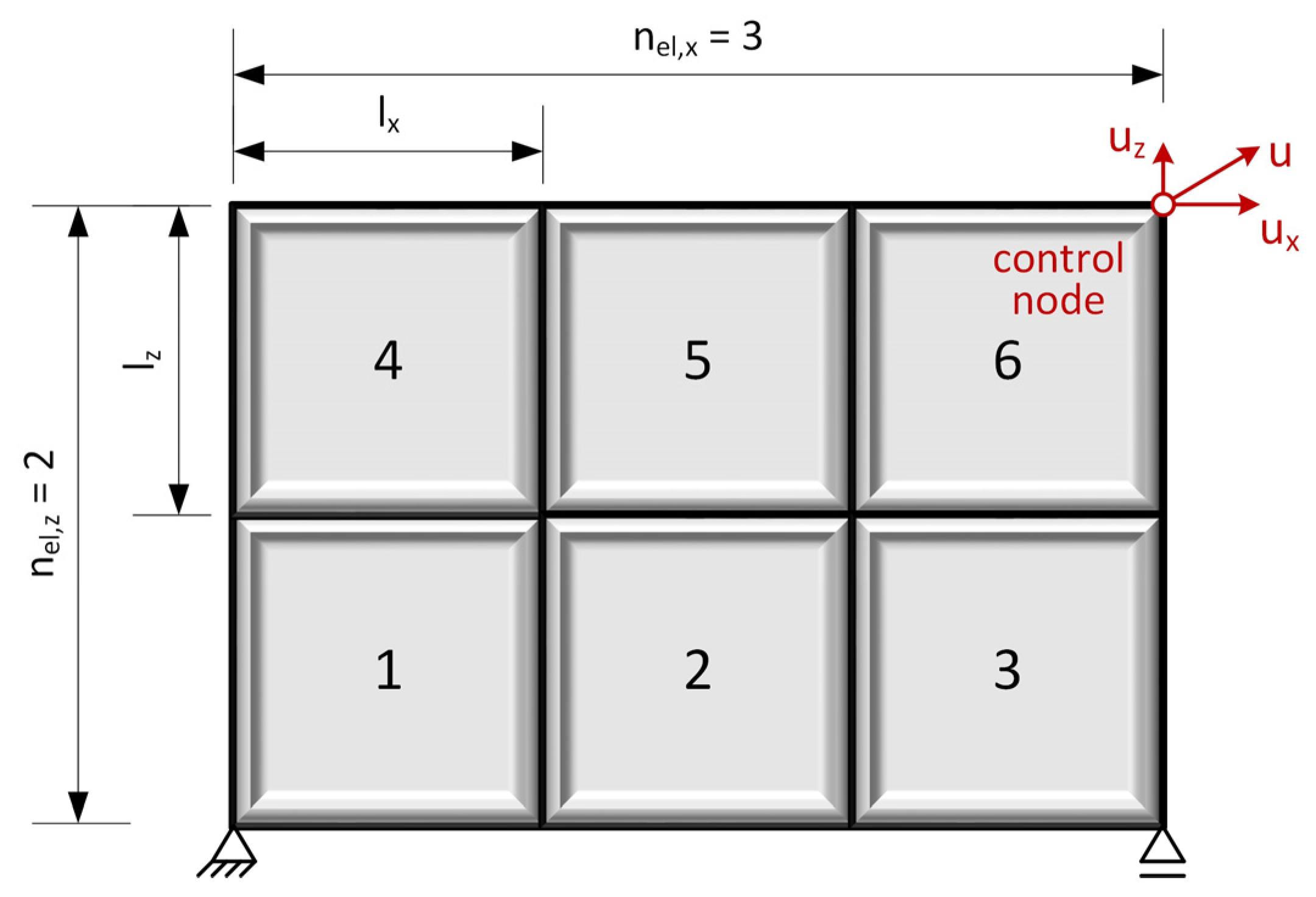
2.3. Extension to (Plane) Structures Consisting of Several Modules—Superposition of Geometric Deviations Due to Temperature Constraints

Planar modular structures are considered next, which are composed of several rectangular finite elements. For convenience, the model is parameterized with respect to the number of modules in horizontal n_el,x and vertical directions n_el,xz as well as for the module dimensions l_x and l_z. Virtually, the system corresponds to a single-span or a wall-like beam, respectively, whereby column-like structures can also be designed depending on the number of modules chosen in the two directions.

To apply geometric deviations according to the temperature equivalent approach introduced in Section 2.2, each module is modeled by a 4-node planar FE with linear shape functions. If the modules would consist of several finite elements with different temperatures, e.g., to model a temperature gradient, unwanted bending occurs. It originates from the forces transferred between the finite elements and would cause unwanted shear stiffening of the module. However and since geometric inaccuracies and their impact on the structure are to be assessed here, this rather coarse discretization with one element per module is seen as sufficiently accurate.

The coefficient of thermal expansion for concrete is set to α_T = 10 × 10⁻⁶ 1/K throughout. For simplicity, the modulus of elasticity is also set constant to 30,000 MPa and representative for a normal-strength concrete. Moreover, the Poisson’s ratio corresponds to ν = 0 to avoid transverse strains and thus orthogonal deformations, which would bias the inaccuracy to be modeled here.

In principle, the deformation can be evaluated on each node or each group of nodes. For the modular structures investigated, this is performed on the node at the top right corner (control node, cf. Figure 4) since it is the most remote from the fixed support. Here, the greatest influences of superimposed deviations due to the inaccuracies of the modules are expected. Horizontal u_x, vertical u_z, and total deformations u are examined. It is worth noting that with another focus, not only deformations but strains, internal forces or other system responses could be used to evaluate sensitivities, too.

Figure 4 shows the conceptual design of the parametrized modular structure exemplary with n_el,x = 3 modules in the x-direction and n_el,z = 2 in the z-direction, i.e., 6 modules in total. The modules are numbered in rows, ascending from bottom left to top right.

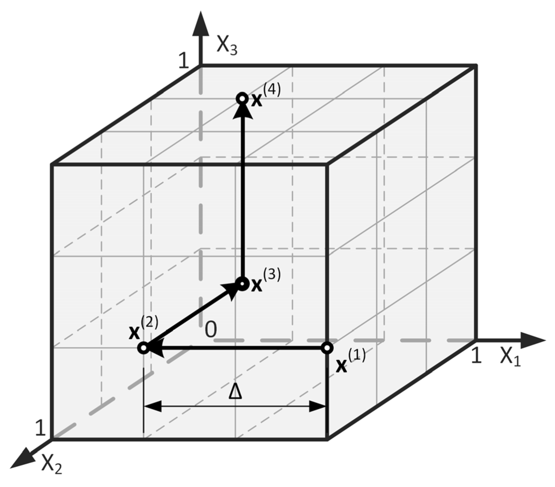
2.4. Sensitivity Analysis of Modular Structures

Sensitivity analysis serves to determine the influence of scattering variables on a system response. In general, local and global techniques are distinguished [41]. The local sensitivity analysis is based on partial derivatives of the system response y according to a parameter x_i* within a set of reference values x_i. The (local) sensitivity S_i with respect to x_i* is numerically obtained as follows:

$$S_{\mathrm{i}}=\frac{y\left(x_1,x_2,\dots , x_{\mathrm{i}}^{\mathrm{*}},\dots , x_{\mathrm{n}}\right)-y\left(x_1,x_2,\dots , x_{\mathrm{i}}^{*}+\mathsf{\Delta }{x}_{\mathrm{i}},\dots , x_{\mathrm{n}}\right)}{\mathsf{\Delta }{x}_{\mathrm{i}}}$$

(4)

Therein, the increment ∆x_i corresponds to the change in the parameter x_i* whose influence is to be analyzed.

Limitation of the local sensitivity analysis lies in the limited value range of parameters, so that possibly decisive regions of the design space might not be examined for their influence. Especially for non-linear models, this can yield insufficient results. Therefore, methods of global sensitivity analysis are recommended, as these allow for variations in the parameters over the entire design space and cover non-linear models as well as enabling the identification of interactions between the parameters.

To quantitatively assess their impact, the scatter of the input variables on the scatter of the system response is examined. Using sampling methods, such as Latin Hypercube Sampling [42,43] or the Sobol’ sequences [44], parameter ranges can be mapped holistically and the scatter can be taken into account via distribution functions. However, for a quantitative analysis, e.g., via quantile values, a large number of evaluations becomes necessary. This often excludes numerical investigations with the finite element method (FEM) due to high computational effort. In comparison to qualitative methods, so-called screening methods [45] require significantly fewer evaluations. Typically, they are used to identify decisive or less relevant parameters, for example, to reduce complex models [46]. Subsequently, a quantitative sensitivity analysis can be carried out in a then reduced design space [41].

For the modular structures investigated here, the elementary effects (EE) method is adapted to identify the modules that have a decisive influence on the superimposed structural inaccuracy. The EE method belongs to the global sensitivity analyses [35] and is used when a too large number of variables does not allow for a more elaborated variance-based sensitivity analysis. It bases on the system response y, e.g., of an FE simulation, which depends on k input parameters. For sampling, the input parameters are successively increased by an increment. Thereby, the k-dimensional design space is built up diametrically. The design space forms—as is usual for sampling methods—a unit space with the limits [0; 1] for each dimension k. Next, the unit space is divided into p-1 intervals of equal size. From this, the increment ∆ can be computed according to [35,47,48]:

$$\mathsf{\Delta }=\frac{p}{2\left(p-1\right)}$$

(5)

The parameter p is an even number and is to be chosen in such a way that ∆ > 0.5 to cover (almost) the entire design space during sampling. The result is a trajectory of k + 1 points describing a path through the k-dimensional unit cube with the diagonal length of ∆√k. Figure 5 shows the trajectory exemplarily for p = 4 (∆ = 2/3) and a dimension of k = 3.

Affine to Equation (4), the (local) sensitivity EE_i of parameter i can be determined according to the change in the system response y due to the increment ∆:

$${EE}_{\mathrm{i}}=\frac{y\left(x_1,x_2,\dots , x_{\mathrm{i}}+\mathsf{\Delta },\dots , x_{\mathrm{k}}\right)-y\left(x_1,x_2,\dots , x_{\mathrm{i}},\dots , x_{\mathrm{k}}\right)}{\mathsf{\Delta }}$$

(6)

To cover the entire unit space, it is advisable to generate several trajectories r. Therefore, a total of r(k + 1) calculations or simulations of y is necessary. According to [36,41], good results are obtained for r = 10 and p = 4.

The random trajectories are generated as follows. A base point x* is created by choosing a random value from the interval [0, 1/(p − 1),2/(p − 1), …, 1 − ∆] for each dimension. x* is then increased by ∆ for one or more parameters and thus forms the starting point x⁽¹⁾. The following points x⁽ⁱ⁺¹⁾ are generated from the previous point x⁽ⁱ⁾ by increasing or decreasing a random parameter j with j = 1, …, k by ∆ until this is completed exactly once for each parameter (cf. Figure 5). All points must lie within the unit space. A numerical implementation in matrix notation is published, for example, in [45].

The sensitivities EE_i are then determined for all trajectories, and the mean μ_i and the standard deviation σ_i are subsequently derived as follows:

$${\mu }_{\mathrm{i}}=\frac{1}{r}\left(E{E}_{\mathrm{i},1}+E{E}_{\mathrm{i},2}+\cdots +E{E}_{\mathrm{i},\mathrm{r}}\right)$$

(7)

$${\sigma }_{\mathrm{i}}=\sqrt{\frac{1}{r-1}\left[{\left(E{E}_{\mathrm{i},1}-{\mu }_{\mathrm{i}}\right)}^2+{\left(E{E}_{\mathrm{i},2}-{\mu }_{\mathrm{i}}\right)}^2+\cdots +{\left(E{E}_{\mathrm{i},\mathrm{r}}-{\mu }_{\mathrm{i}}\right)}^2\right]}$$

(8)

The mean thus corresponds to the average influence of the parameter i. The standard deviation provides information on non-linearities or interactions between the input parameters [41]. According to [36], it is recommended to use the mean μ_i* of the absolute values |EE_i| to avoid sign-related misinterpretation.

$${\mu }_{\mathrm{i}}^{\mathrm{*}}=\frac{1}{r}\left(\left|E{E}_{\mathrm{i},1}\right|+\left|E{E}_{\mathrm{i},2}\right|+\cdots +\left|E{E}_{\mathrm{i},\mathrm{r}}\right|\right)$$

(9)

This ensures that significant influences that take on partially positive or negative values and thus might negate each other are identified, too.

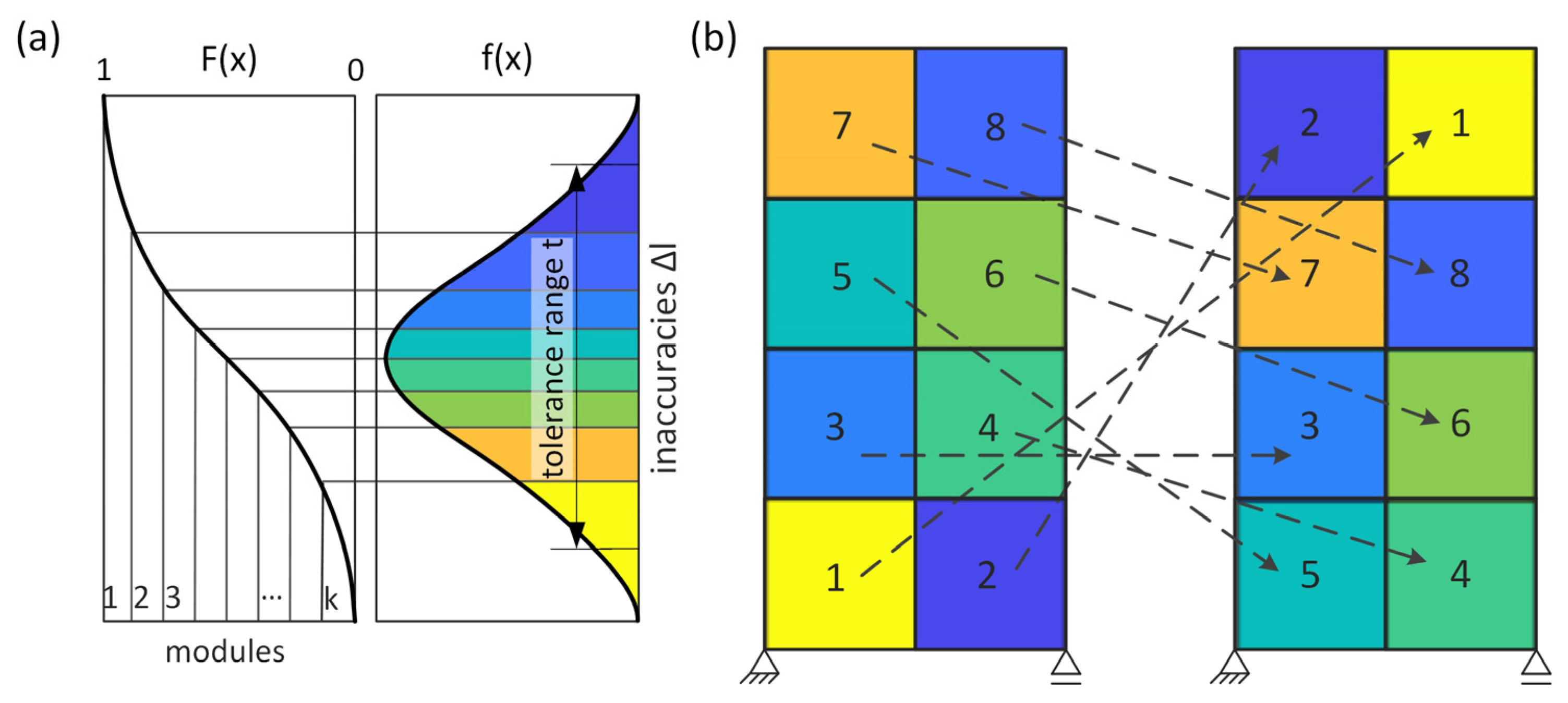
2.5. Sensitivity-Based Permutation of Modules

Once the decisive positions of modules in the structure have been identified by means of the EE method, it is favorable to arrange them regarding the weighting of their average influence μ_i⁽*⁾. All modules together define a construction kit that contains as many modules as necessary for the structure sought. Here, the structure is designed in such a way that each module can be interchanged with any other (cf. Figure 4). No limitations arise from individual bearing capacities that might be incorporated defining two or more different module types. Then of course, the type of module would affect the sensitivities, too. Just for the sake of simplicity when identifying the sensitive positions here, an equal type of module has been used to compute the EEs. The placement strategy is as follows: module positions that possess high μ* are assigned to modules that have low deviations. This means that modules with low inaccuracy are assigned to positions with high impact and vice versa.

For illustration, a construction kit is formed containing the k modules of the structure in Figure 6. The geometric inaccuracies of the modules scatter in the tolerance range t. LHS of the inaccuracies ∆l is performed to cover the design space completely. For precast concrete elements, the tolerance range corresponds to two times the standard deviation of a Gaussian distribution [38]. This construction kit is then used to place the modules and compute the resulting structural deformations. These deformations are compared for random placement versus sensitivity-based permutation. Qualitative evaluation employs repeated simulation. n_sim kits of the same tolerance range are generated, the modules placed and the resulting structural inaccuracies evaluated.

3. Results

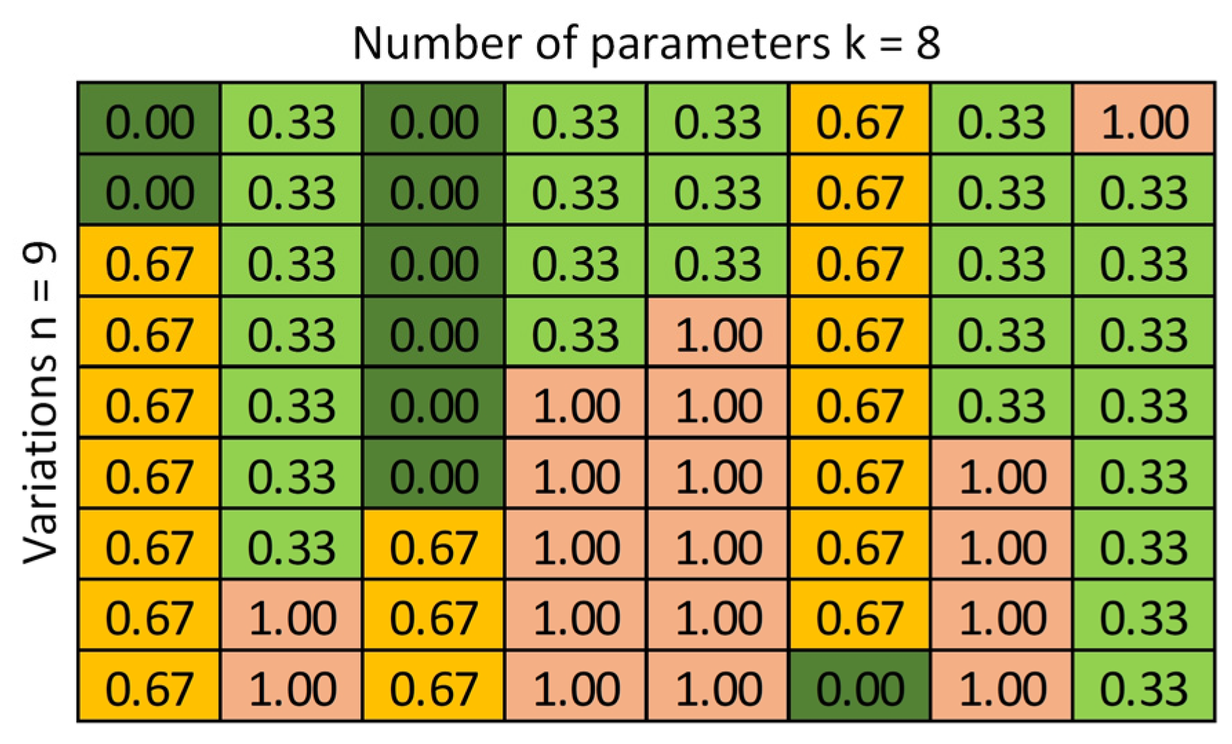
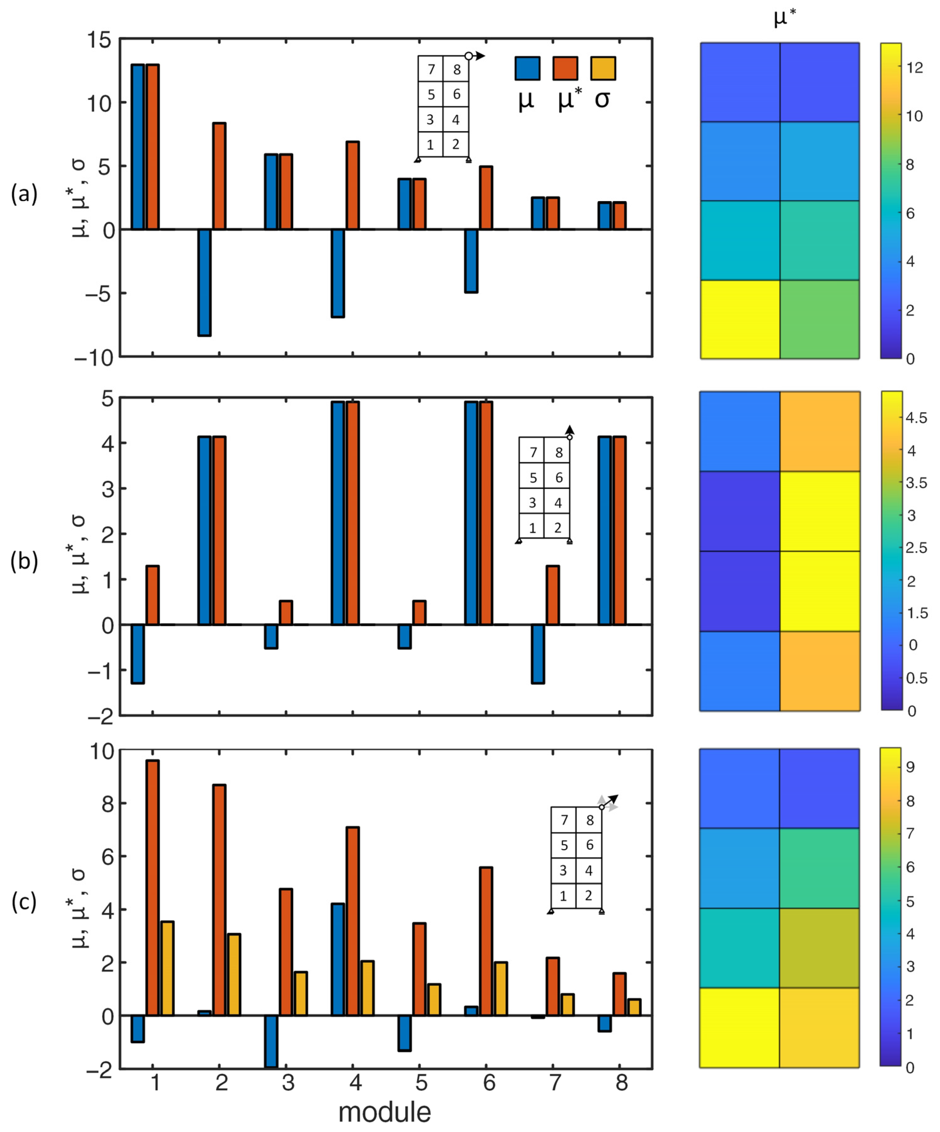
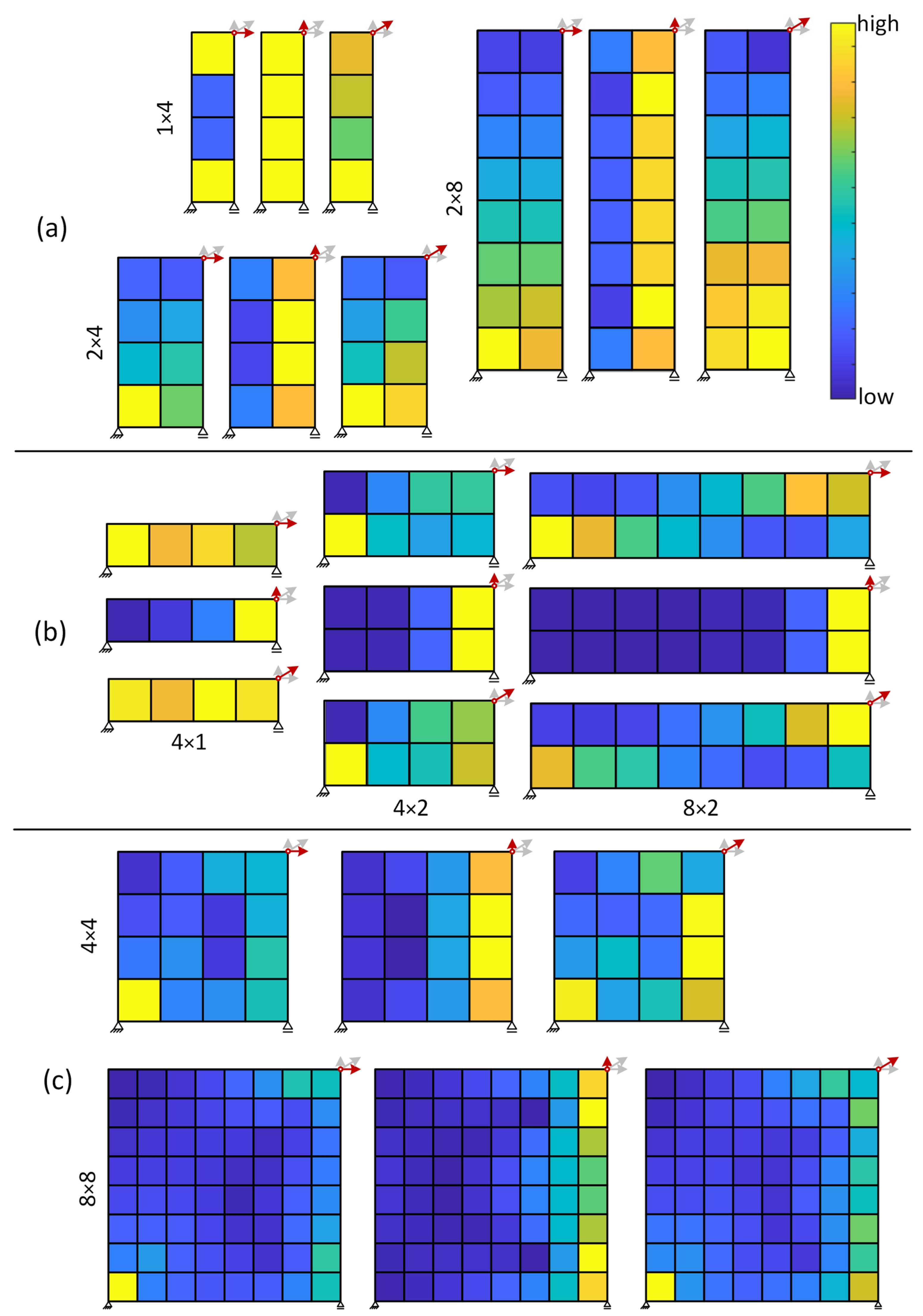
3.1. Sensitivity Analysis

3.1.1. Sampling of Inaccuracies

To evaluate the impact of individual module inaccuracies on the entire structure, the equivalent temperature constraints must be sampled according to the procedure outlined in Section 2.2. Therefore, the trajectory through the unit space is first constructed as a function of the parameter k, which corresponds to the number of modules in the overall structure (n_el,x × n_el,z). With p = 4, the interval [0, 1] is divided into p − 1 = 3 subintervals. The increment corresponds to ∆ = 2/3 (cf. Equation (5)). Figure 7 shows the trajectory for a structure with k = 8 modules in matrix notation. Between each of the n = 9 variations, only one entry is altered by ∆. All possible values of the sampling points, i.e., 0, 0.33, 0.67, and 1, for the variations are color-coded to illustrate this graphically. As recommended in Section 2.4, r = 10 trajectories are investigated in total, which leads to n_sim = r(k + 1) = 90 simulations in the example.

The matrix entries are then interpreted as probabilities P and matched to the tolerance range of the geometric inaccuracies ∆l. For concrete, a tolerance range of twice the standard deviation is chosen as discussed above (cf. Section 2.1). The modules here are assumed to possess a tolerance of ± 2 mm, which represents the production-induced tolerance [38]. Matching associates the lower limit 0 with a probability of P = 0.02275 and the upper limit 1 with P = 0.97725 of the Gaussian distribution. This yields geometric deviations of ∆l = [−2, −0.41, 0.41, 2] mm at the sampling points of the unit trajectory. Obviously, the increment in the unit space is not proportional to the change in ∆l.

Next, ∆l is converted into equivalent temperature constraints ∆T. For the sake of simplicity, constant equivalent temperature constraints ∆T and thus equal deviations in both directions on quadratic modules are applied. Consequently, α_T,x equals α_T,z and ∆T can be determined from Equation (3), just as a function of the module size l.

3.1.2. Sensitivity Analysis of Exemplary Modular Structures

Sensitivities are analyzed on the example of structures with a few square modules of the same edge lengths l_x = l_z = 0.5 m for convenience. To cover diversity, the selection includes 1D column- or beam-like structures with a minimum number of n_elx = n_elz = 4 elements and square 2D wall-like structures with up to n_elx = n_elz = 64 modules. Thus, the sampling of the EE method requires 50 to 650 simulations. Figure 8 shows the corresponding temperature constraint ∆T (left) and the resulting absolute deformations u (right) exemplarily for a modular structure of 2 × 4 modules. For the module size of 0.5 m and the maximum tolerances of ±2 mm, ∆T varies between −400 K and 400 K. Maximum deformation occurs in the top right corner of the column-like structure due to the tilt.

The elementary effects of this structure are shown in Figure 9 for the horizontal u_x (a), vertical u_z (b), and total deformations u (c) at the control node. For both the horizontal and vertical deformations, the standard deviation for each module is zero, which indicates an additive model (no interaction). Only for the total deformations do the EE scatter (σ ≠ 0). This is because absolute deformations are always positive, which is interpreted as a non-linear effect.

Regarding the horizontal displacements of the structure (Figure 9a, left) the influence of the modules increases continuously from bottom to top. The modules on the left above the fixed support always have more impact μ* than the others. Moreover, all modules on the right—except for the top row—exhibit a negative impact μ. This means that positive inaccuracies have a negative impact on the horizontal deviation at the control node and vice versa. This just does not apply to the upper row, since the module at the control node has a direct effect on the horizontal deviation. For the vertical displacement at the control node (Figure 9b, left), the modules on the right have the greatest influence. In comparison, the modules on the left have a small influence μ, which is also negative throughout.

The elementary effects μ and μ* show the same absolute value per module for the horizontal as well as for vertical deformations. This is no longer the case for the total deformations (Figure 9c). Here, some μ* are significantly bigger than the associated μ, so that misinterpretation might happen when analysis is just based on μ. Therefore, μ* is used in the remainder as the essential characteristic of the analysis of the influence of the module position.

μ* is separately visualized by color coding the modules in Figure 9 (right). The influence μ* on the total deformation also increases from bottom to top, similar to the horizontal deformations. The module at the fixed support possesses maximum influence since it contributes significantly to the inclination of the structure due to the bearing concept chosen. Simultaneously, the increased influence of the right-hand side modules, as identified in (b), can be observed, which have an almost additive effect on the vertical and thus the total deformations. However, the horizontal displacements due to inclination are decisive for this structure since the maximum influences of the horizontal deformations dominate the vertical ones.

In the following, the absolute influences μ* for different structures are investigated. Figure 10 shows these in color coding for horizontal, vertical, and total displacements, whereby the influence is colored qualitatively from low or none (blue) to high (yellow). The types of structure cover columns (a), beams (b), and walls (c).

As is shown in Figure 9, modules at the support of column-like structures have the greatest impact on deflection. This trend is confirmed in Figure 10a for structures with more modules over the height. The higher the position of a module, the less influence it has, except for vertical deformations. Here, the entire column of modules below the control node is most influential. In general, this picture is also confirmed for columns with only one module across the width. However, the support then acts like a clamp and causes uniform impact of all elements against vertical deformation. Then, the vertical direction even dominates and leads to an almost equal weighting of all modules that prevails for the overall deformations.

A similar result is observed on modular beams with one module in the z-direction. Here, μ* for the horizontal displacement is almost the same for all modules. However, since the static system is a simply supported beam, bending effects can occur due to the varying temperature constraints which affect the modules’ influence and, hence, not all are identified as equal. For beam-like structures with two modules over the height (n_el,z = 2), a higher influence of the module at the fixed support on the horizontal and total deformations is observed. In the lower row, the influence decreases continuously from the support to the control node, while it is exactly the opposite in the top row. Differently, the vertical deformations are significantly influenced just by the modules at the right edge, i.e., those below the control node, as already observed for the column-like structures.

A similar observation is made for wall-like structures (c). The module at the fixed support is decisive for the total and especially for the horizontal deformations. Vertical deformations are again dominated by the modules below the control node at the right edge. By contrast, wide areas inside the structure, especially for large structures (8 × 8 modules), have hardly any influence.

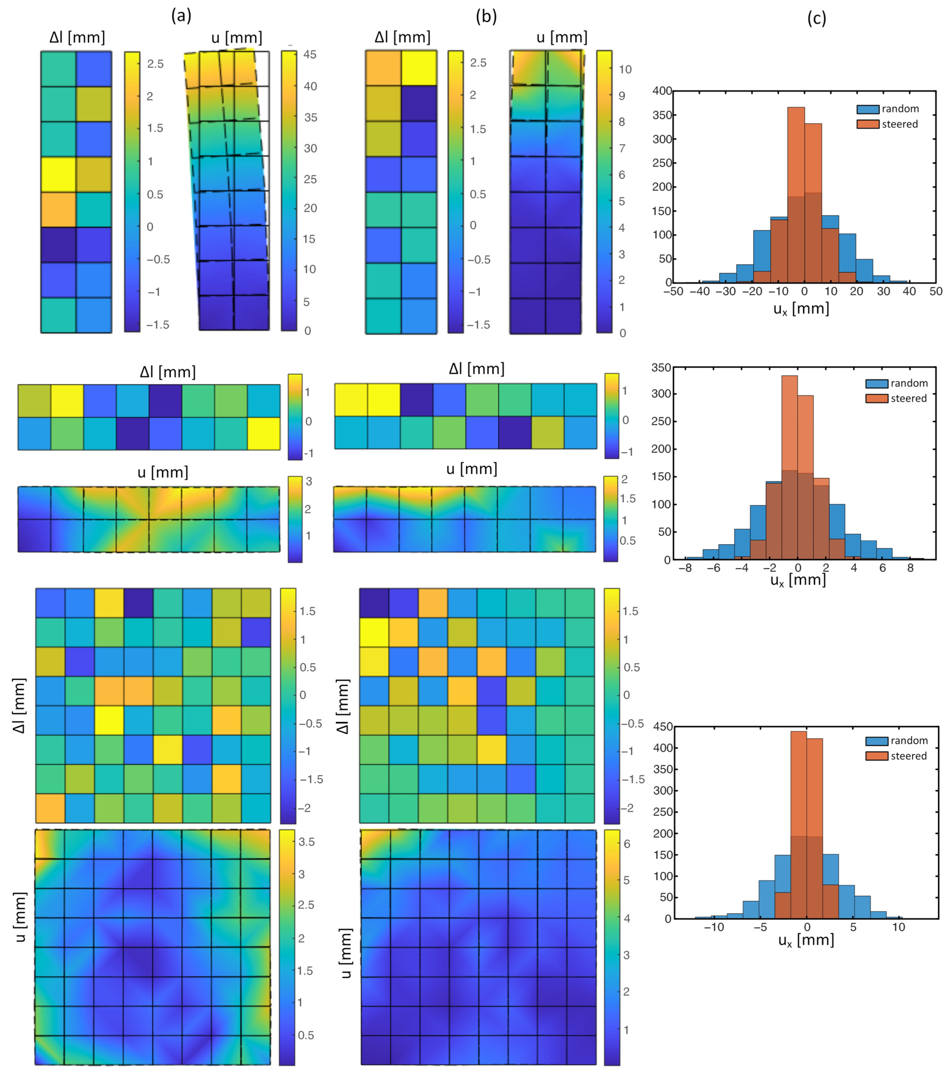
3.2. Sensitivity-Based Permutation to Reduce Structural Inaccuracies

As said, the EE method belongs to the qualitative methods and primarily serves for screening. Nevertheless, it quantifies the impact of individual modules regarding their mean (absolute) influence. It is therefore investigated how the structural deformations can be improved if modules with individual inaccuracy are placed in the structure with respect to their influence μ*. Here, μ* is applied on the total deformation u. To capture the diversity of structures, a column (2 × 8), a beam (8 × 2), and a wall with 8 × 8 modules are analyzed. All have been assessed with respect to their sensitivities (cf. Figure 10).

For qualitative evaluation, a total of n_sim = 1000 simulations is carried out for each structure. The inaccuracies cover the tolerance range of +/−2 mm, which describes the previously defined confidence interval of 95.45% (2σ) of a Gaussian distribution. Using LHS, the inaccuracies of the individual modules are sampled. Thereby, values greater than the tolerance range of 2 mm can appear but with low probability (cf. Figure 6a). Finally, the sampled ∆l are converted to ∆T, as proposed above (cf. Section 2.5).

Each simulation hereby comprises two calculations, i.e., one for an initial, random placement and one for a permutated one of the same modules just weighted by μ*. The results are visualized in Figure 11 for the column-like (top), beam-like (center) and wall-like structures (bottom). Shown are the basic module inaccuracies ∆l and resulting total structural deformations u from random sampling (a), sensitivity-based placement by permutation (b), and the histograms of the horizontal deformations u_x at the control node for all n_sim simulations (c).

Due to inclination, the column-like structure exhibits the greatest horizontal deformation. The beam-like and wall-like structures show less deformation, as the inaccuracies of the modules tend to partly compensate for each other. For all structures, however, a reduction in the deformations at the control node is achieved for the steered placement, as shown in Figure 11c in the example of u_x. In relation to the overall structure, however, controlled placement can result in locally higher deformations, as can be observed in the wall-like structure, for example. Since the evaluation of the modules’ influence on the deformations was performed with respect to the control node, high deformations due to permutation are observed in the upper left edge, too. They even exceed the maximum deformations of a random placement. In general, however, reduced deformations are obtained over wide parts of the structures for all three cases investigated. For the column-like and beam-like structure, the total deformation is, thereby, usually reduced (cf. Figure 11).

Basic statistics of the horizontal u_x, vertical u_z, and absolute deformations u, like the mean values (mean) and standard deviations (std), are summarized in

Table 1. Evaluation of the deformations in the control node for different modular structures as mean value (mean) and standard deviations (std) for a random placement and sensitivity-based permutation of the modules according to Figure 11.

Type of Modular Structure	Number of Modules		Deformation [mm]
			ux				uz				u
			Random		Steered		Random		Steered		Random		Steered
	nel,x	nel,z	Mean	Std	Mean	Std	Mean	Std	Mean	Std	Mean	Std	Mean	Std
Column	2	8	0	13.38	−0.37	6.74	0	3.59	0.14	3.42	11.38	7.88	6.44	3.96
Beam	8	2	0	2.76	0	1.32	0	1.82	0.03	0.7	2.9	1.58	1.26	0.78
Wall	8	8	0	3.54	0.01	1.17	0	2.85	−0.02	0.94	3.93	2.29	1.32	0.71

. As expected, u_x and u_z have zero means for random placement of the modules, which slightly differs for the permutation approach. Moreover, the absolute total deformation u is always positive, and so is the mean. Maximum mean deformation and scatter occur on the column-like structure. The beam- and wall-like structures show lower deformation. In a comparison of the two, it is slightly higher for the wall.

Throughout, standard deviations and means are significantly reduced with sensitivity-based permutation. Regardless of whether components or total quantities are considered, mean and standard deviations of wall-like structures are reduced to 33%. For column- and beam-like structures, standard deviations in the (horizontal) x-direction and in total are reduced to 50%. Again, the (vertical) z-direction is special. While the standard deviation of columns is nearly not affected at all, it is reduced to 38% for beams. Due to the one dominant direction of columns and beams, the decrease in mean deformation is lower compared to walls (43% and 57%, respectively).

4. Discussion

4.1. Modeling Inaccuracies with Temperature Constraint

Geometric inaccuracies can be modeled in a simplified way by means of equivalent temperature constraints ∆T. These are then applied on elements or modules, respectively, within an FE environment. For plane elements, almost any deviations can be induced via different temperature constraints at the nodes, whereby the average deformations per spatial direction of neighboring nodes result. Since different deviations in the spatial directions are controlled by the corresponding thermal expansion coefficients α_T,x and α_T,z, the deviations for each node of an element must be equally proportional. The following deformation can be set:

• Constant deformation in one direction.
• Constant, proportional deformations for both directions in the plane.
• Linearly variable deformation in one direction.
• Linearly variable, proportional deformation in both directions.

Completely arbitrary deviations of the nodes are impossible to capture by this approach. Further limitations result from the static system of the modular structure that is to be investigated or more precisely from its degree of static determination. If it is statically determined, the deformations due to temperature constraints superimpose additively. If the system is (internally) static-overdetermined, module inaccuracies are still additive in the spatial directions—as revealed by means of the sensitivity analysis—yet a quantitative evaluation of the structural deformation becomes infeasible due to constraint-induced eigenstresses. In assembly, these stresses must be absorbed by the modules if possible. If not, tolerance-compensating joints that are to be derived with respect to the specific structure and joining method must be implemented. However, in this case, computationally intensive modeling approaches, such as direct kinematics, are preferred [49]. In general, the presented method with equivalent temperature constraints is sufficient to simulate qualitative deviations in structures to identify modules whose inaccuracy has a significant effect on the overall structural inaccuracy using sensitivity analysis.

4.2. Sensitivity-Based Permutation Approach

Using the EE method, decisive parameters can be identified for a certain system response with a maximum of 650 simulations for the largest modular structure investigated here. In contrast, other sensitivity analysis techniques, e.g., sensitivity-based total effects [50], require N·(k + 2) simulations, in which the sample size N varies between a few hundreds to thousands and more depending on the model under investigation [41]. Already with N = 100, which is still much too low for reliable results [46], the EE method requires more than 10 times fewer simulations. This is why the EE method is adapted for the analysis of relevant module positions that mainly cause deformations on an overall structure. Here, the structural inaccuracy was determined for the superimposed deformations at a predefined control node. The evaluation of the module impact thus only applies to the examined deviations at this location. It has been shown that for the selected node, which is located most remotely from the fixed support, the deformations are greatly reduced by a permutation of the modules weighted by the mean absolute influence μ*. This holds true for different types of modular structures, i.e., plane modular columns, beams, and walls consisting of quadratic modules. Furthermore, deformations over large areas of the structure are also counterbalanced. In construction, modules with high deviations that exceed tolerance requirements can be placed in areas of low influence so that overall structural tolerance is still satisfied. Thereby, expensive and emitting reworking or even disposal of these modules is avoided, helping to ensure a sustainable design. However, areas with low influence might get worse and reveal higher deformations. Then, only single modules might be replaced with newly built, more accurate ones. For a holistic approach, further control points or even sets of nodes can be defined. But, too many control points with conflicting sensitivities could prevent optimal rearrangement, and then the effort of steered placement would no longer be worthwhile. However, the specific optimization for a certain node of the structure that requires high accuracy, e.g., for connections [9], is more appropriate. The approach shown here is useful for this. Using the EE method, the positions that require precise modules can be identified with minimal computational effort by means of FEA. These specific regions or points can then be communicated to the quality management within a BIM (building information modeling) environment or digital twin framework [51,52], so that tolerance requirements are controlled in the production process, e.g., using laser scanning, to guarantee fast construction [53,54].

5. Conclusions

This paper presents a sensitivity-based approach using the EE-method to identify module positions in modular structures that are highly influential on the overall structural inaccuracy. To cover diversity, column-, beam-, and wall-like structures whose modules have individual geometric inaccuracies that interact holistically are investigated. The following conclusions are drawn:

• Versatile but not arbitrary geometric deviations can be modeled through the equivalent temperature approach. In an FE environment, corresponding temperature constraints are directly applied to the nodes of the modules. But, deviations are not explicitly prescribable at the nodes, just indirectly for a module. Nevertheless, this approach is considered sufficiently accurate to model geometric inaccuracies within modular structures.
• Deviations in (internally) static-overdetermined modular structures cause eigenstresses which must be absorbed by the modules, in assembly.
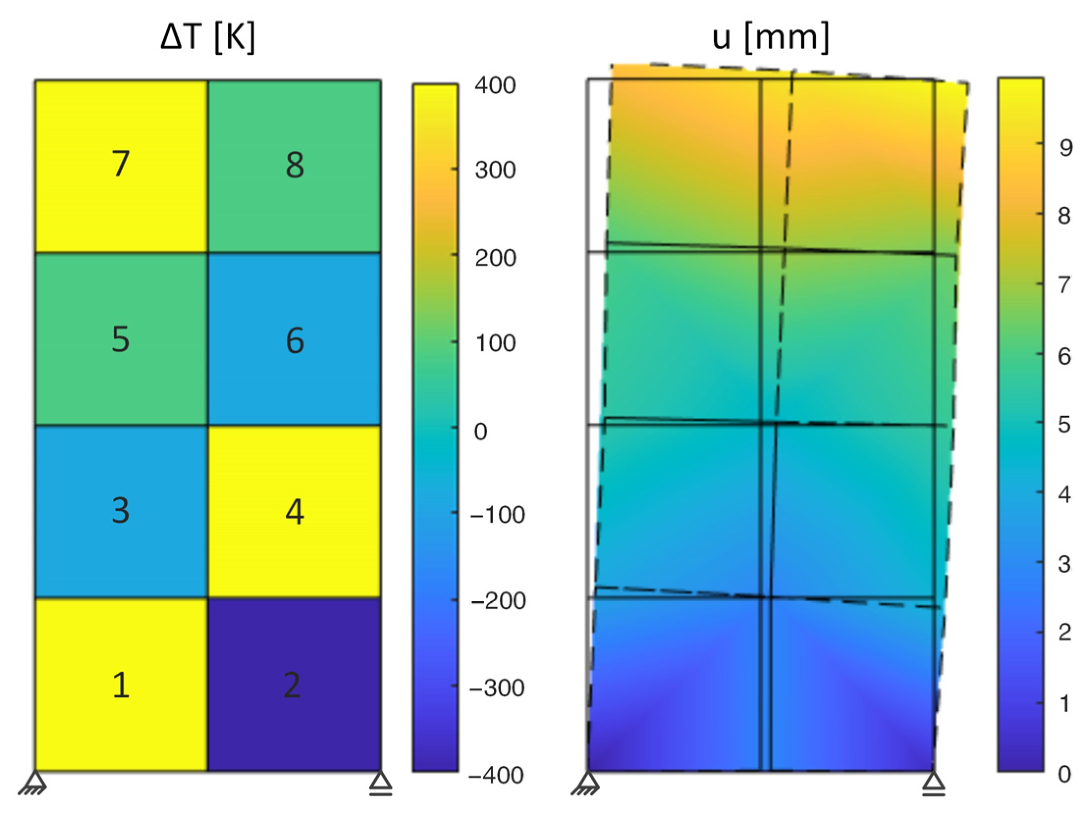
• In the chosen statically determinate system, which resembles a simply supported beam, the horizontal deformations of the investigated structures dominate. For column-like modular structures, this bearing configuration results in particularly high deformations due to inclination.
• Modules at the fixed support always exhibit the greatest impact on the absolute deformation at the control node regardless of the type of structure. The impact on the structural inaccuracy decreases the higher the position of the module for column-like structures.
• Sensitivity-based permutation with the EE method reduces the total deformations at the control node by at least 43% on average. The scatter of deformation is also significantly reduced by at least 50% for columns and beams or 69% for walls. Modules with high inaccuracies that otherwise would be disposed of due to tolerance requirements can still be used in areas of low influence. A resource-efficient and sustainable design is ensured.
• The sensitivity-based permutation approach can easily be adapted to evaluate other system responses rather than deformations, e.g., strains, stresses, or internal forces.
• With respect to sustainability, this method provides two crucial advantages. First, the reworking and disposal of modules can be reduced or even avoided due to the tolerance-compensating placement. Second, the modular design enables the exchange of modules in the structure, e.g., to extend the service lifetime of the whole structure without deconstruction. Hereby, the approach of temperature constraints can be adapted to minimize the eigenstresses of the module for exchange by temperature induction of the adjacent modules, which will be the focus of future investigations.

References

1. Kolbeck, L.; Kovaleva, D.; Manny, A.; Stieler, D.; Rettinger, M.; Renz, R.; Tošić, Z.; Teschemacher, T.; Stindt, J.; Forman, P.; et al. Modularisation Strategies for Individualised Precast Construction—Conceptual Fundamentals and Research Directions. Designs 2023, 7, 143. [Google Scholar] [CrossRef]
2. Steinle, A.; Bachmann, H.; Tillmann, M. Precast Concrete Structures, 2nd ed.; Ernst & Sohn: Berlin, Germany, 2019; ISBN 978-3-433-03225-1. [Google Scholar]
3. Oettel, V.; Empelmann, M. Structural behavior of profiled dry joints between precast ultra-high performance fiber reinforced concrete elements. Struct. Concr. 2019, 20, 446–454. [Google Scholar] [CrossRef]
4. Manny, A.; Stempniewski, L.; Albers, A.; Simons, K. Conceptual design and investigation of an innovative joint for the rapid and precise assembly of precast UHPC elements. Eng. Struct. 2022, 265, 114454. [Google Scholar] [CrossRef]
5. Kim, Y.-J.; Chin, W.-J.; Jeon, S.-J. Interface Shear Strength at Various Joint Types in High-Strength Precast Concrete Structures. Materials 2020, 13, 4364. [Google Scholar] [CrossRef] [PubMed]
6. Baghdadi, A.; Heristchian, M.; Kloft, H. Connections placement optimization approach toward new prefabricated building systems. Eng. Struct. 2021, 233, 111648. [Google Scholar] [CrossRef]
7. Baghdadi, A.; Heristchian, M.; Ledderose, L.; Kloft, H. Experimental and numerical assessment of new precast concrete connections under bending loads. Eng. Struct. 2020, 212, 110456. [Google Scholar] [CrossRef]
8. Bischof, P.; Mata-Falcón, J.; Burger, J.; Gebhard, L.; Kaufmann, W. Experimental exploration of digitally fabricated connections for structural concrete. Eng. Struct. 2023, 285, 115994. [Google Scholar] [CrossRef]
9. Rajanayagam, H.; Poologanathan, K.; Gatheeshgar, P.; Varelis, G.E.; Sherlock, P.; Nagaratnam, B.; Hackney, P. A-State-Of-The-Art review on modular building connections. Structures 2021, 34, 1903–1922. [Google Scholar] [CrossRef]
10. Thai, H.-T.; Ngo, T.; Uy, B. A review on modular construction for high-rise buildings. Structures 2020, 28, 1265–1290. [Google Scholar] [CrossRef]
11. Rettinger, M.; Prziwarzinski, A.; Meyer, M.; Kolbeck, L.; Tošić, Z.; Hückler, A.; Lordick, D.; Borrmann, A.; Haist, M.; Lohaus, L.; et al. Modulare Fußgängerbrücken aus seriell hergestellten Betonfertigteilen. Beton Stahlbetonbau 2023, 118, 803–814. [Google Scholar] [CrossRef]
12. Teschemacher, T.; Bletzinger, K.-U. CAD-integrated parametric modular construction design. Eng. Rep. 2023, 5, e12632. [Google Scholar] [CrossRef]
13. Stieler, D.; Schwinn, T.; Menges, A. Automatisierte Bauteilzerlegung für Betonfertigteile aus additiv hergestellten Schalungen. Beton Stahlbetonbau 2022, 117, 324–332. [Google Scholar] [CrossRef]
14. Markowski, J.; Meyer, M.; Haist, M.; Lohaus, L. Duktilitätssteigernde Bewehrungssysteme für fließgefertigte Stabelemente aus UHFB. Beton Stahlbetonbau 2022, 117, 998–1007. [Google Scholar] [CrossRef]
15. Blandini, L.; Kovaleva, D.; Haufe, C.N.; Nething, C.; Nigl, D.; Nitzlader, M.; Smirnova, M.; Strahm, B.; Bosch, M.; Funaro, D.; et al. Leicht bauen mit Beton—ausgewählte Forschungsarbeiten des ILEK—Teil 2: Strukturleichtbau. Beton Stahlbetonbau 2023, 118, 320–331. [Google Scholar] [CrossRef]
16. Gappmaier, P.; Reichenbach, S.; Kromoser, B. Automated Production Process for Structure-Optimised Concrete Elements. In Building for the Future: Durable, Sustainable, Resilient; Ilki, A., Çavunt, D., Çavunt, Y.S., Eds.; Springer Nature Switzerland: Cham, Switzerland, 2023; pp. 1577–1585. ISBN 978-3-031-32510-6. [Google Scholar]
17. Stoiber, N.; Kromoser, B. Topology optimization in concrete construction: A systematic review on numerical and experimental investigations. Struct Multidisc Optim 2021, 64, 1725–1749. [Google Scholar] [CrossRef]
18. Stindt, J.; Forman, P.; Mark, P. Influence of Rapid Heat Treatment on the Shrinkage and Strength of High-Performance Concrete. Materials 2021, 14, 4102. [Google Scholar] [CrossRef] [PubMed]
19. Schoening, J.; Della Pietra, R.; Hegger, J.; Tue, N.V. Verbindungen von Fertigteilen aus UHPC. Bautechnik 2013, 90, 304–313. [Google Scholar] [CrossRef]
20. Shahtaheri, Y.; Rausch, C.; West, J.; Haas, C.; Nahangi, M. Managing risk in modular construction using dimensional and geometric tolerance strategies. Autom. Constr. 2017, 83, 303–315. [Google Scholar] [CrossRef]
21. Liu, Y.; Yao, F.; Ji, Y.; Tong, W.; Liu, G.; Li, H.X.; Hu, X. Quality Control for Offsite Construction: Review and Future Directions. J. Constr. Eng. Manag. 2022, 148, 03122003. [Google Scholar] [CrossRef]
22. Ma, Z.; Liu, Y.; Li, J. Review on automated quality inspection of precast concrete components. Autom. Constr. 2023, 150, 104828. [Google Scholar] [CrossRef]
23. Du Plessis, A.; Boshoff, W.P. A review of X-ray computed tomography of concrete and asphalt construction materials. Constr. Build. Mater. 2019, 199, 637–651. [Google Scholar] [CrossRef]
24. Mendricky, R. Determination of measurement accuracy of optical 3D scanners. MM Sci. J. 2016, 2016, 1565–1572. [Google Scholar] [CrossRef]
25. Sun, K.; Tran, T.-H.; Guhathakurta, J.; Simon, S. FL-MISR: Fast large-scale multi-image super-resolution for computed tomography based on multi-GPU acceleration. J. Real-Time Image Proc. 2022, 19, 331–344. [Google Scholar] [CrossRef]
26. Ballast, D.K. Handbook of Construction Tolerances, 2nd ed.; Wiley: Hoboken, NJ, USA, 2007; ISBN 978-0-471-93151-5. [Google Scholar]
27. Rausch, C.; Nahangi, M.; Haas, C.; Liang, W. Monte Carlo simulation for tolerance analysis in prefabrication and offsite construction. Autom. Constr. 2019, 103, 300–314. [Google Scholar] [CrossRef]
28. Long, H.; Luo, X.; Liu, J.; Dong, S. The Analysis and Application of Installation Tolerances in Prefabricated Construction Based on the Dimensional Chain Theory. Buildings 2023, 13, 1799. [Google Scholar] [CrossRef]
29. Talebi, S.; Koskela, L.; Tzortzopoulos, P.; Kagioglou, M. Tolerance Management in Construction: A Conceptual Framework. Sustainability 2020, 12, 1039. [Google Scholar] [CrossRef]
30. Wagner, R.; Kuhnle, A.; Lanza, G. Optimising Matching Strategies for High Precision Products by Functional Models and Machine Learning Algorithms. In Proceedings of the 7th WGP-Jahreskongress, Aachen, Germany, 5–6 October 2017; Schmitt, R.H., Schuh, G., Eds.; pp. 231–239. [Google Scholar]
31. Kaveh, A.; Zolghadr, A. Meta-heuristic methods for optimization of truss structures with vibration frequency constraints. Acta Mech 2018, 229, 3971–3992. [Google Scholar] [CrossRef]
32. Alberdi, R.; Khandelwal, K. Comparison of robustness of metaheuristic algorithms for steel frame optimization. Eng. Struct. 2015, 102, 40–60. [Google Scholar] [CrossRef]
33. Nigdeli, S.M.; Bekdaş, G.; Yang, X.-S. Metaheuristic Optimization of Reinforced Concrete Footings. KSCE J. Civ. Eng. 2018, 22, 4555–4563. [Google Scholar] [CrossRef]
34. Stindt, J.; Frey, A.M.; Forman, P.; Mark, P.; Lanza, G. CO2 reduction of resolved wall structures: A load-bearing capacity-based modularization and assembly approach. Eng. Struct. 2024, 300, 117197. [Google Scholar] [CrossRef]
35. Morris, M.D. Factorial Sampling Plans for Preliminary Computational Experiments. Technometrics 1991, 33, 161. [Google Scholar] [CrossRef]
36. Campolongo, F.; Cariboni, J.; Saltelli, A. An effective screening design for sensitivity analysis of large models. Environ. Model. Softw. 2007, 22, 1509–1518. [Google Scholar] [CrossRef]
37. de Zanet, G.; Viquerat, A. Screening methods for sensitivity analysis applied to thin composite laminated structures. Thin-Walled Struct. 2022, 172, 108870. [Google Scholar] [CrossRef]
38. Forman, P.; Mark, P. Fertigungstoleranzen von Betonfertigteilen für die modulare Bauweise. Beton Stahlbetonbau 2022, 117, 286–295. [Google Scholar] [CrossRef]
39. Bazant, Z.P. Criteria for Rational Prediction of Creep and Shrinkage of Concrete. In SP-194: The Adam Neville Symposium: Creep and Shrinkage-Structural Design Effects; American Concrete Institute: Indianapolis, IN, USA, 2000; ISBN 9780870316920. [Google Scholar]
40. Toutenburg, H.; Knöfel, P. Six Sigma: Methoden und Statistik für die Praxis, 2nd ed.; Springer: Berlin/Heidelberg, Germany, 2008; ISBN 9783540851370. [Google Scholar]
41. Saltelli, A.; Ratto, M.; Andres, T. Global Sensitivity Analysis: The Primer, 1st ed.; Wiley-Interscience: Hoboken, NJ, USA, 2008; ISBN 0470059974. [Google Scholar]
42. Helton, J.C.; Davis, F.J. Latin hypercube sampling and the propagation of uncertainty in analyses of complex systems. Reliab. Eng. Syst. Saf. 2003, 81, 23–69. [Google Scholar] [CrossRef]
43. McKay, M.D.; Beckman, R.J.; Conover, W.J. Comparison of Three Methods for Selecting Values of Input Variables in the Analysis of Output from a Computer Code. Technometrics 1979, 21, 239–245. [Google Scholar] [CrossRef]
44. Sobol’, I. On the distribution of points in a cube and the approximate evaluation of integrals. USSR Comput. Math. Math. Phys. 1967, 7, 86–112. [Google Scholar] [CrossRef]
45. Sanio, D.; Obel, M.; Mark, P. Screening methods to reduce complex models of existing structures. In Proceedings of the 17th International Probabilistic Workshop (IPW), Edinburgh, UK, 11–13 September 2019; pp. 51–56. [Google Scholar]
46. Sanio, D.; Ahrens, M.A.; Mark, P. Lifetime predictions of prestressed concrete bridges—Evaluating parameters of relevance using Sobol’ indices. Civ. Eng. Des. 2022, 4, 143–153. [Google Scholar] [CrossRef]
47. Campolongo, F.; Saltelli, A. Sensitivity analysis of an environmental model: An application of different analysis methods. Reliab. Eng. Syst. Saf. 1997, 57, 49–69. [Google Scholar] [CrossRef]
48. Campolongo, F.; Tarantola, S.; Saltelli, A. Tackling quantitatively large dimensionality problems. Comput. Phys. Commun. 1999, 117, 75–85. [Google Scholar] [CrossRef]
49. Singh, R.; Kukshal, V.; Yadav, V.S. A Review on Forward and Inverse Kinematics of Classical Serial Manipulators. In Advances in Engineering Design; Rakesh, P.K., Sharma, A.K., Singh, I., Eds.; Springer: Singapore, 2021; pp. 417–428. ISBN 978-981-33-4017-6. [Google Scholar]
50. Saltelli, A.; Annoni, P.; Azzini, I.; Campolongo, F.; Ratto, M.; Tarantola, S. Variance based sensitivity analysis of model output. Design and estimator for the total sensitivity index. Comput. Phys. Commun. 2010, 181, 259–270. [Google Scholar] [CrossRef]
51. Kosse, S.; Vogt, O.; Wolf, M.; König, M.; Gerhard, D. Digital Twin Framework for Enabling Serial Construction. Front. Built Environ. 2022, 8, 864722. [Google Scholar] [CrossRef]
52. Kosse, S.; Vogt, O.; Wolf, M.; König, M.; Gerhard, D. Requirements Management for Flow Production of Precast Concrete Modules. In Advances in Information Technology in Civil and Building Engineering; Skatulla, S., Beushausen, H., Eds.; Springer International Publishing: Cham, Switzerland, 2024; pp. 687–701. ISBN 978-3-031-35398-7. [Google Scholar]
53. Kalasapudi, V.S.; Tang, P.; Zhang, C.; Diosdado, J.; Ganapathy, R. Adaptive 3D Imaging and Tolerance Analysis of Prefabricated Components for Accelerated Construction. Procedia Eng. 2015, 118, 1060–1067. [Google Scholar] [CrossRef]
54. Kim, M.-K.; Wang, Q.; Park, J.-W.; Cheng, J.C.; Sohn, H.; Chang, C.-C. Automated dimensional quality assurance of full-scale precast concrete elements using laser scanning and BIM. Autom. Constr. 2016, 72, 102–114. [Google Scholar] [CrossRef]
Figure 1. Procedure of the sensitivity-based placement strategy.
Sustainability 16 03016 g001
Figure 2. Modeling geometric deviations for a truss element: (a) 1D module with initial deviations, (b) schema of the FE, (c) temperature constraints, (d) resulting deviations.
Sustainability 16 03016 g002
Figure 3. Modelling geometric deviations for plane FE: (a) 2D module with initial deviations, (b) FE net, (c) temperature constraints, (d) resulting deformations; from top to bottom: biaxial constant, uniaxial constant, uniaxial variable, (almost) arbitrary at the nodes (red – positive temperatures or deformations, blue – negative temperatures or deformations).
Sustainability 16 03016 g003
Figure 4. Parametrized modular structure of a wall-like beam made of 3 × 2 modules. Control node to evaluate the superimposed deformations located at the top right corner.
Sustainability 16 03016 g004
Figure 5. Exemplary trajectory in a 3-dimensional unit space with p = 4 and k = 3.
Sustainability 16 03016 g005
Figure 6. (a) Latin Hypercube Sampling of geometric inaccuracies with respect to a tolerance range, (b) random placement and sensitivity-based permutation of modules.
Sustainability 16 03016 g006
Figure 7. Trajectory in the unit space for k = 8 parameters and n = 9 variations in matrix notation.
Sustainability 16 03016 g007
Figure 8. Temperature constraints (left) and corresponding absolute deformations (right) of a simply supported column made from 2 × 4 square modules.
Sustainability 16 03016 g008
Figure 9. Elementary effects μ, μ*, and σ for the modular structure according to Figure 8 (left) with additional absolute effect μ* of module inaccuracies (right) with respect to horizontal (a), vertical (b), and absolute deformations (c).
Sustainability 16 03016 g009
Figure 10. Qualitative elementary effects μ* of module positions within modular structure as columns (a), beams (b), and walls (c) with respect to horizontal, vertical, and absolute deformation.
Sustainability 16 03016 g010
Figure 11. Geometric deviations ∆l and resulting deformations u for random placement (a) and a sensitivity-based permutation of the modules (b) with corresponding deformations in horizontal direction ux as bar plots at the control node (c).
Sustainability 16 03016 g011