The Impact of Official Promotion Incentives on Urban Ecological Welfare Performance and Its Spatial Effect

Abstract

Economic growth, environmental protection, and welfare improvement are closely related to local officials. Therefore, exploring the paths that affect ecological welfare performance (EWP) from the perspective of official promotion incentives has certain practical significance. EWP is an indicator that measures the welfare relationship between ecological resource inputs and outputs, reflecting the sustainable development status of a region. First, considering the background of the dual carbon goals, the EWPs of 284 cities from 2007 to 2020 were measured by constructing an indicator system and using the super-SBM-DEA method. Second, by constructing a theoretical framework of “official promotion incentives-fiscal responsiveness-EWP”, we empirically tested the impact and mechanism of official promotion incentives on urban EWP; finally, based on regional and official age heterogeneity, we explored the differential impacts of official promotion incentives on urban EWPs. The results show that official promotion incentives inhibit the improvement of urban EWP by reducing financial responsiveness; in terms of spatial spillovers, under three types of spatial weight matrices, promotion incentives for officials in neighboring areas can significantly improve the EWPs of local cities. From the perspective of regional differences, official promotion incentives in the eastern region significantly improved urban EWP, official promotion incentives in the western and northeastern regions significantly inhibited urban EWP, and official promotion incentives in the central region had no significant impact on urban EWP. From the perspective of official age, local officials aged 53 and 54 intensified the inhibitory effect of promotion incentives on urban EWP. By constructing a theoretical framework and empirical testing, this paper provides theoretical support and empirical evidence for the impact of official promotion incentives on urban EWP. The results help to understand the relationship between official promotion incentives and sustainable development, and promotes sustainable urban development.

1. Introduction

The concept of ecological welfare originates from the steady-state economy proposed by Herman Daly [1]. It is used to measure the improvement level of social welfare under a certain consumption of natural resources, aiming to achieve the most welfare with the least consumption of ecological resources. Finding a development path with low carbon, low pollution, and high welfare has become the key to China’s economic and social development. The concept of ecological welfare meets the needs of “environment-economy-welfare” coupling and can measure the strong sustainable development level of a country or region, reflecting local ecological governance and people’s happiness [2].

The academic research on EWP has expanded from performance measurement to the influencing factors [3] and convergence of EWP [4]. The current research is mostly analyzed from the perspectives of technological progress, the level of opening up and green development [5], industrial structure, and the level of environmental regulation [6], etc., and mainly uses multiple linear regression methods and spatial econometric models. Local officials play an important and complex role in economic transformation and social development. Local officials have the power to allocate resources, which has an impact on economic growth, environmental pollution, and the improvement of residents’ welfare. Promotion incentives are the biggest incentives for officials, which is in line with their “political person” attributes. Although some research has explored the impact of official promotion incentives on economic growth, environmental pollution, or welfare, the impact of local official promotion incentives on the comprehensive indicator of urban EWP has been overlooked. Based on this, this study raises the following research questions: Does official promotion incentives have impact on urban EWP? Are there spatial spillover effects? Through what mechanism do official promotion incentives affect urban EWP? Will urban location and official age lead to differentiated effects of official promotion incentives on EWP?

Our study may contribute to the existing literature in two ways. First, at the research perspective level, it explores the mechanism affecting urban EWP from the perspective of official promotion, enriching relevant research on factors and mechanisms affecting EWP. Second, at the data level, instead of using the existing EWP research that focuses on the provincial or partial city scale, this article extends the data to 284 city scales across the country in 2020. It is helpful to analyze the EWP of Chinese cities from a smaller research scale. Compared with previous studies related to officials, this article has the characteristics of a relatively new sample period. The official data used in this article have been updated to 2019 based on the data published by Jiang’s team as of 2015. At the level of fiscal responsiveness data, it took several months to collect detailed data through the CIEC database, China Municipal Statistical Yearbook, China Regional Economic Statistical Yearbook (2000–2014), and municipal statistical bulletins, etc.

The structure of this article is as follows: Section 2 summarizes and reviews the literature on the impact of official promotion incentives on economic growth, environmental protection, and welfare improvement; Section 3 is the research design section, which introduces the research methods, models, and variable meanings used; Section 4 includes the empirical analysis, in which the benchmark regression results, the robustness test, the mechanism test, and the heterogeneity test are analyzed; and Section 5 is the conclusion and policy implications.

2. Literature Review

In China, Zang and Zhu were the first to introduce the concept of ecological welfare, believing that EWP is the efficiency of converting natural consumption into welfare levels [7,8], which can measure whether a country or region is approaching or moving away from sustainable development [9]. When measuring EWP, scholars often use methods such as questionnaires, ratios, stochastic frontier analysis (SFA), and data envelopment analysis (DEA). Specifically, Long believe that subjective welfare is psychologically perceived. Welfare can be measured through questionnaires, such as exercise, relaxation, commuting, work, and social interaction and there are few applications in the field of welfare measurement. With the development and maturity of the concept of ecological welfare, research on measuring objective EWP has increased year by year, mainly including the ratio, SFA, and DEA methods [10]. The ratio method uses the ratio of welfare level and ecological footprint to measure EWP [11]. For example, Zhu used the ratio of the human development index (HDI) to the ecological footprint to measure the EWP of 124 countries and regions [11]. After that, the DEA method has been the most widely used. Long used energy, water resources, and land consumption as input indicators, industrial wastes as undesirable output indicators, economic development as intermediate indicators, the human development index and subjective satisfaction as output indicators, and used the DEA method to measure the EWP of 35 cities in China [12].

As research continues to deepen, some scholars have begun to explore the factors that affect EWP, mainly focusing on multi-factor research. Some scholars have also begun to deeply explore the mechanism of various influencing factors on EWP. For example, Guo has focused on exploring the impact of environmental regulations on EWP. The influencing mechanism of urban EWP in the Yangtze River Economic Belt has deepened this research. The absence of government entities and the lack of functional mechanisms in the study of urban EWP provides an opportunity to further supplement and expand the research. China’s marketization process has obvious government leadership. As the makers, implementers, and supervisors of economic policies, local government officials play an active role [13]. Since the 1980s, the assessment standards for local officials in China have changed from traditional political indicators to economic indicators with GDP growth rate. Therefore, for a long time, official promotion incentives have been the most important factor in promoting China’s rapid economic growth. Although the existing literature has not directly studied the relationship between official incentives and urban EWP, there are many studies on the impact of official incentives on the economy, environment, or welfare improvement (the three dimensions of ecological welfare). In view of this, this study will review the research related to official incentives and the connotation of ecological welfare (economic growth, environmental protection, and welfare improvement).

In terms of research on official incentives and economic growth, the phenomenon of officials’ promotion of economic development to the “promotion tournament” promoted rapid local economic growth [14]. Zhang believes that the “performance view” of local officials “competing for growth” is the most effective incentive mechanism to promote China’s economic growth [15]. Currently, as China’s economy enters a new stage of high-quality development, scholars have begun to discuss the relationship between official promotion and the quality of economic development. For example, some studies have found that official promotion incentives have a positive impact on high-quality economic development [16], while some studies suggest the opposite [17]. Therefore, the relationship between official promotion and high-quality economic development remains to be further verified. In the context of the relationship between official promotion and economic growth, scholars have begun to explore the impact of individual characteristics of officials on economic growth. Some studies have found that individual characteristics such as officials’ academic qualifications are positively correlated with economic growth [18]. In addition, officials’ personal abilities and development prospects also have a positive motivating effect on regional economic growth.

The impact of official promotion incentives on environmental pollution can be roughly divided into “exacerbation theory” and “inhibition theory”. The “exacerbation theory” believes that incentives for official promotion will aggravate environmental pollution. In order to obtain political promotion, local officials may ignore local environmental protection, resulting in the problem of “growth for promotion and pollution for growth” [19]. Specifically, the GDP-oriented cadre assessment intensifies environmental pollution through two paths: First, by lowering environmental standards. In order to pursue economic performance, officials will not hesitate to lower environmental standards and environmental supervision to attract more high-pollution workers. High emissions and high energy consumption have been caused by the investment in building factories locally [20]; secondly, environmental protection expenditures have been squeezed out. In order to increase economic growth, local officials have invested in a large amount of infrastructure construction, further squeezing out ecological and environmental protection expenditures, and making it difficult to control environmental pollution [20]. The “inhibition theory” is mainly argued from the perspective of accountability. As age increases, the probability of officials being promoted decreases, but the cost of environmental accountability continues to increase, so older officials are more motivated to control environmental pollution [21].

In recent years, China’s financial power has been further transferred to the central government, while power in areas such as science, education, culture, and health have been continuously transferred to local governments. The provision of public services has become a matter of “conscience” for governments at all levels. Some scholars have begun to delve into the relationship between official promotion incentives and public service supply, and have formed two main views: one view is that official promotion incentives have a negative impact on public service supply, such as the “economic man” characteristics of government officials, further expanding the effect of the non-equalization of urban and rural public services in China [22]; another view is that official promotion incentives have a significant positive impact on the sharing of public goods and public services [23]. In addition, some scholars have found that the relationship between official promotion incentives and public service supply is not in an “either/or” relationship; different characteristics of officials will also show certain differences in the supply of public services [24].

However, there are few studies on how local official promotion incentives affect EWP. Due to the influence of local official behavior on both macroeconomic and resource allocation, officials’ behavior is largely influenced by promotion incentives, which have an impact on economic growth, environmental pollution, and welfare improvement. The characteristics of officials, such as age and education level, may also affect EWP. Due to China’s vast territory and differences in regional economic development levels, there is also heterogeneity in official promotion incentives across different regions.

In terms of research content, research on urban EWP mainly focuses on building an indicator system and measuring performance. First, there are many studies exploring the impact of multiple factors on urban EWP, and few articles are in-depth. Existing studies have mainly considered the impact of official promotion incentives on regional economic development and environmental protection, paying less attention to the impact of comprehensive indicators such as EWP. Nowadays, people have diverse needs, especially in large developing countries like China. As income levels increase, residents’ needs have evolved from food and clothing in the early stages to ecological environment, cultural tourism, and other activities [25]. The existing literature has failed to explore the influencing factors on urban EWP from the official promotion incentives perspective. Second, at the level of indicator system construction, many scholars use environmental pollution as an input indicator. This study refers to existing research and includes environmental pollution as an undesirable output in an urban EWP indicator system [26,27], taking into account the background of carbon peak and carbon neutrality, incorporating carbon dioxide emissions into the indicator system, and further improving the construction of the indicator system. Third, in terms of research scale, existing studies mostly focus on the provincial scale and regional scale, and some studies focus on the national level, but few studies focus on the urban scale. In view of this, this article uses panel data from 2007 to 2020 on 284 cities as a sample, uses welfare expenditure structure as an intermediate variable, explores the mechanism and spatial spillover effect of official promotion incentives on urban EWP, and expands official incentive mechanisms that influence strong sustainable development and refine the research scale of EWP.

3. Research Design

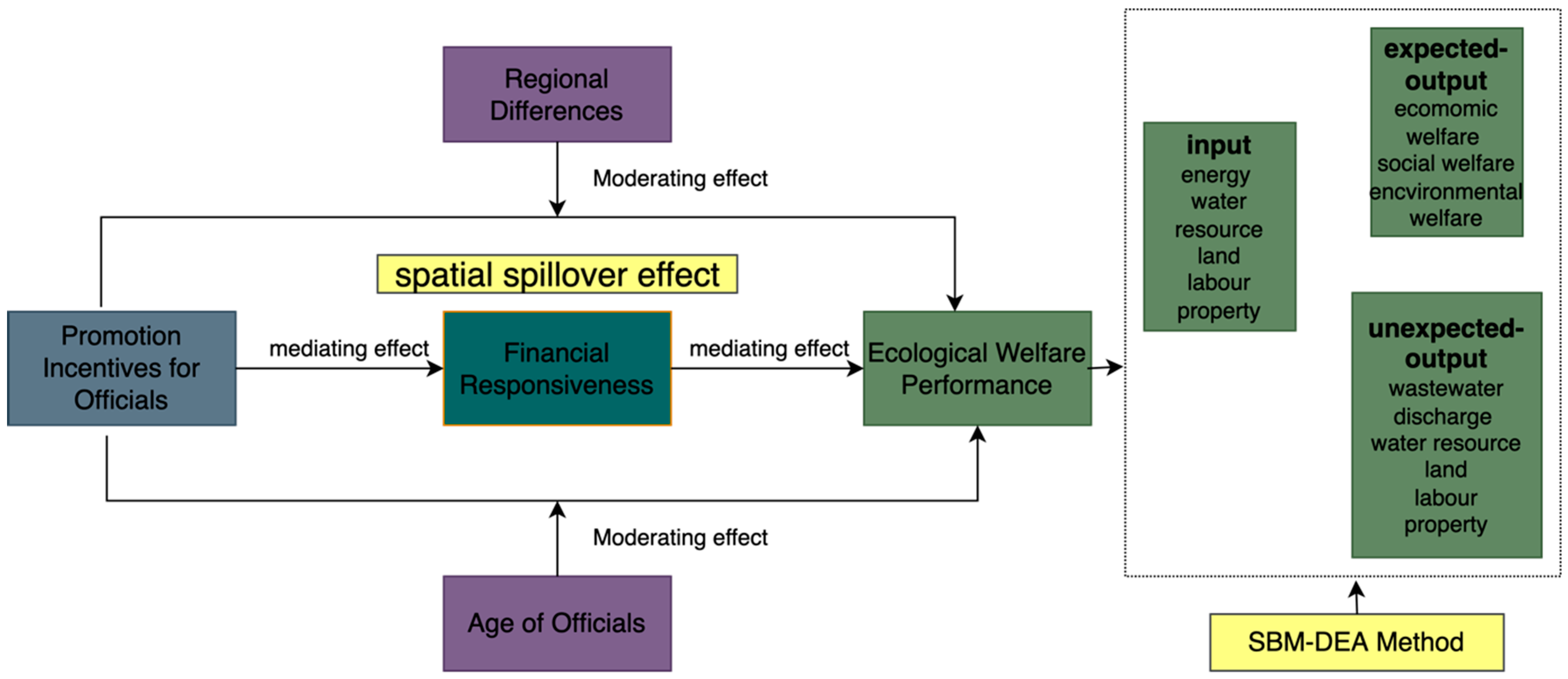
3.1. Super-SBM-DEA Model

The DEA method was first proposed by Charnes in 1978 and can solve the problem of inconsistent units of resource input and environmental pollution output [28]. The SBM-DEA model was based on relaxation variables and non-radial non-angle proposed by Tone in 2001 [29]. It was chosen in this study to measure the EWP of Chinese cities using the Super-SBM-DEA model proposed by Tone in 2002 due to the inability to rank multiple effective decision-making units [30]. Assuming there are n decision units in the production system, and each decision unit has three input–output variables, namely input, desirable output, and undesirable output, the specific calculation formula is shown in Equation (1):

$$\begin{gathered} {min\rho }^{*}=\frac{1+\frac{\frac{1}{m}\sum _{m=1}^M{s}_m^x}{x_{jm}^t}}{1-\frac{1}{l+h}\left(\sum _{l=1}^L\frac{s_l^y}{y_{jl}^t}+\frac{\sum _{h=1}^H{s}_h^b}{b_{jh}^t}\right)} \\ \mathrm{s}.\mathrm{t}.\left\{\begin{array}{c}{x}_{jm}^t\ge {\displaystyle \sum _{j=1,j\ne 0}^n}{\lambda }_j^t{x}_{jm}^t+s_m^x\\ y_{jt}^t\ge {\displaystyle \sum _{j=1,j\ne k}^n}{\lambda }_j^t{y}_{jl}^t-s_l^y\\ b_{jh}^t\ge {\displaystyle \sum _{j=1,j\ne k}^n}{\lambda }_j^t{b}_{jh}^t+s_h^b\\ {\lambda }_j^t\ge 0,s_m^x\ge 0,s_l^y\ge 0,j=1,\dots ,n\end{array}\right. \end{gathered}$$

(1)

Among them, ${\rho }^{*}$ is the EWP, where $x_j^t, y_j^t,$ and $b_j^t$, respectively, represent the input, desirable output, and undesirable output values of ${DMU}_j$ during period t; $m, l, and h$ represent the number of inputs, desirable outputs, and undesirable outputs, respectively; The relaxation variables of input, desirable output, and undesirable output are represented by $s_m^x$, $s_l^y, and s_h^b$, respectively; $\lambda$ is the weight vector of the decision-making unit.

3.2. Research Methods and Model Setting

EWP includes three levels: economic growth, environmental protection, and welfare improvement. Considering that economic growth and environmental protection have spatial spillover effects, traditional measurement methods may lead to estimation errors. The spatial econometric analysis method breaks the assumption that samples are independent of each other and can avoid the errors of traditional measurement to a certain extent. Therefore, this article intends to use a spatial econometric model to explore the impact and mechanism of official promotion incentives on urban EWP. The settings of the spatial autoregressive model are as follows:

$${EWP}_{i,t}=\alpha +\rho \sum _{j=1}^N{W}_{ij}{EWP}_{j,t}+\beta {Prom}_{i,t}+\varphi X_{i,t}+{\phi }_i+{\eta }_t+{\epsilon }_{i,t}$$

(2)

Among them, ${Prom}_{i,t}$ is the official promotion incentive, ${EWP}_{i,t}$ is the city’s EWP, ρ measures the spatial spillover effect of city j on city i’s EWP, and $W_{i,j}$ is the spatial weight. In the matrix, the spatial error model is set as follows:

$$\begin{gathered} {EWP}_{i,t}=\alpha +\beta {Prom}_{i,t}+\varphi X_{i,t}+{\phi }_i+{\eta }_t+{\mu }_{i,t} \\ {\mu }_{i,t}=\lambda \sum _{j=1}^N{W}_{ij}{\mu }_{i,t}+{\epsilon }_{i,t} \end{gathered}$$

(3)

${\mu }_{i,t}$ is the disturbance term, λ is the spatial dependence coefficient of the disturbance term, and the other variables have the same meaning as above.

The spatial Durbin model is set as follows:

$${EWP}_{i,t}=\alpha +\rho {\sum }_{j=1}^N{W}_{ij}{EWP}_{j,t}+{\beta Prom}_{i,t}+\gamma {\sum }_{j=1}^N{W}_{ij}{Prom}_{j,t}+\varphi X_{i,t}+\sigma {\sum }_{j=1}^N{W}_{ij}{X}_{j,t}+{\phi }_i+{\eta }_t+{\epsilon }_{i,t}$$

(4)

γ is the effect of promotion incentives of officials in neighboring areas on the EWP of local cities, where σ is the effect of control variables in neighboring areas on the EWP of local cities, and the meanings of the other variables are the same as above.

3.3. Variable and Data Description

Dependent variable: EWP. The DEA method can solve the problem of inconsistent units of multiple resource inputs and environmental pollution output without considering specific production functions, weights, and parameters. Therefore, this study chose the SBM-DEA model proposed by Tone to measure the EWP of Chinese cities.

Table 1. Urban EWP measurement indicators.

Dimension	First-Level Index Layer	Second-Level Index Layer	Third-Level Index Layer	Unit
Input indicators	Resources input	Energy consumption	Electricity consumption of the whole society	Billion kilowatt hours
		Water consumption	Water consumption	Billion tons
		Land resource consumption	Built-up area	Square kilometers
		Labor input	Number of environmental protection personnel	People
		Property investment	Urban municipal public facilities construction fixed asset investment	Ten thousand yuan
			Environmental protection expenditure	Ten thousand yuan
Output indicators	Desirable-output	Economic welfare	Regional GDP	Billion
		Environmental welfare	Green space	Hectare
		Social Welfare	Average years of education per capita 1	Year
			Number of health personnel	People
			The actual urban road area at the end of the year	Ten thousand square meters
	Undesirable-output 2	Waste water disposal	Industrial wastewater discharge	10,000 tons
		Smoke and dust emissions	Industrial smoke and dust emissions 3	Ton
		Exhaust emissions	Industrial sulfur dioxide emissions	Ton
			Carbon dioxide emissions 4	Ton

¹ The average years of education per capita is expressed using the calculation method of the United Nations Development Program:$AEY=\frac{6\times P_1+9\times P_2+12\times P_3+16\times P_4}{p_1+p_2+p_3+p_4}$, $P_1$, $P_2$, $P_3$, $P_4$ represent the number of students in primary school, junior high school, high school, and university respectively. ² In order to ensure the accuracy of EWP measurement, this paper reduces the dimensionality of undesired outputs and incorporates them into performance measurement by synthesizing the environmental pollution index. ³ Smoke and dust emissions. The statistical report on smoke and dust emissions in 2020 has been adjusted. The statistical caliber has been changed from that during the 13th Five-Year Plan period, and smoke and dust emissions have been renamed particulate matter. ⁴ Incorporating carbon dioxide emissions into undesired outputs is in line with the context of carbon peaking and carbon neutrality. Some scholars have tried to use luminous light data to invert the carbon emission footprint of administrative areas at or below the municipal level. However, this method has certain flaws due to the flaws of the light data itself, such as background noise and discontinuity. The CO₂ emissions data for this article are taken from the Center for Global Environmental Research’s Open Access Fossil Fuels (ODIAC) dataset. ODIAC first introduced the combination of nighttime lights and emission-location profiles of individual power plants to estimate the spatial extent of fossil fuels, with a spatial resolution of 1 KM and a unit of t/KM². The dataset is generated by combining multi-source nighttime light data, global point source data, and ship or aircraft tracking. The data can represent carbon dioxide emissions at global, regional, and city levels and meet the requirements of large-scale and long-term series. By clipping, synthesizing, and extracting China’s carbon emission grid data, China’s urban carbon dioxide emissions from 2007 to 2019 were obtained, and the trend function was used to supplement the emissions in 2020.

shows the indicator system used to measure EWP.

Independent variable: Some of the literature believes that the most direct incentive faced by officials is promotion incentives (Prom), which can reflect the “political person” attributes of government officials [31]. This study uses the economic growth targets set by local governments as proxy variables for official promotion incentives [32] and the main reasons are the following:

(1) Economic growth goals are clear and comparable. Although local government performance appraisals are becoming increasingly diversified and local governments are paying more attention to environmental protection and welfare improvement, economic development is still the focus of local governments [33]. Economic growth targets can be observed in horizontal local government competition, which can reflect the intensity of competition among local governments [34].

(2) Official promotion incentives are widespread and binding on official behavior. Throughout the party and government system, including party committees and administrative departments, economic growth targets will be announced in party congress work reports, government work reports, and development planning documents, thereby constraining official behavior. This is reflected in the fact that government work reports often set economic growth targets while attaching constraints. In addition to the specific numerical value of the economic growth target, strong constraints such as “above”, “ensure”, “reach”, and “strive for” will also be added [35].

(3) It can influence official behavior. In the official promotion tournament mode, the economic growth goal plays a role in motivating officials [36]. The central government controls lower-level officials to complete their goals by directly linking officials’ goal completion with career prospects and official promotions [37,38]. Officials who successfully complete their goals are more likely to be promoted, while officials who fail to complete their goals will lose promotion opportunities or even suffer penalties such as dismissal. Completing the goals set by higher-level governments has become the bottom line for lower-level governments [39]. China’s fiscal decentralization system gives local officials relatively extensive resource control rights and administrative decision-making powers, which gives local officials stronger intervention and leadership capabilities in the economic operations of their jurisdictions. In order to achieve economic growth goals and obtain political promotion, local officials will use the resources at their disposal to intervene in economic operations to achieve their goals.

In summary, this study uses the economic growth targets in the statistical bulletins of each city as a proxy variable for official promotion incentives. Considering that China’s economy was affected by the COVID-19 epidemic in 2020, the central government did not set economic growth targets, so this study excludes the 2020 data. By collecting government work reports from Chinese cities from 2007 to 2019, we extracted the economic growth targets of 284 cities, and obtained a total of 3692 samples.

Intermediary variable: Fiscal responsiveness (Response) is the government’s response to residents’ preferences and is closely related to the improvement of EWP. Yin et al. made a detailed proof of welfare expenditures (the ratio of science, education, culture, health, etc., to total fiscal expenditures) as a proxy variable for fiscal responsiveness [40]; this article will not go into details here. The governing preferences of local officials can be transmitted to the macroeconomy through changes in expenditure structure, thereby affecting local economic growth, environmental governance, and welfare level [41]. Therefore, this study collected data on science expenditures, education expenditures, social security and employment expenditures, and medical health and family planning expenditures in 284 cities from 2007 to 2019. Since this study included environmental protection expenditures in the construction of the dependent variable index system. In order to avoid endogeneity, only the above four types of expenditures are included when calculating the proportion of welfare expenditures, and environmental protection expenditures are not included.

Control variable selection: ① Financial development level (Finan). The essence of finance is to integrate a large amount of idle funds in society, convert funds from savings into long-term investment, ease corporate financing constraints, and enhance the sustainability of corporate innovation [42]. Improving the performance of urban ecological welfare requires the coordinated improvement of economic growth and environmental protection. Financial development can provide financial support for economic growth and environmental protection, promote rapid economic development, and improve the level of environmental protection, thereby affecting the EWP. We use the balance of deposits and loans and the proportion of GDP (%) to measure the level of financial development.

② Industrial structure (Stru2). Different industrial structures correspond to different economic growth and pollution levels. According to general rules, the total volume of the secondary industry is often the largest in the industrialization stage, and the technological progress of the manufacturing industry in the secondary industry is significantly faster than that of the service industry, but the proportion of the secondary industry being higher means serious environmental pollution [43]. Therefore, industrial structure will have an impact on urban EWP. This study uses the proportion of the total output value of the secondary industry in GDP (%) to measure the industrial structure.

③ Innovation level (Tec). As the driving force of economic growth gradually shifts from factor-driven to technology-driven, innovation has become the main driving force of urban development and the embodiment of the country’s core competitiveness. Innovation can promote the city’s connotative growth [44], and then have an impact on the city’s EWP. This study uses the number of patents to measure the level of innovation (the number of patents is logarithmically processed).

④ Level of opening up (Openess). Foreign investment creates more job opportunities and promotes economic growth. In addition, foreign-funded enterprises have also transformed China’s growth momentum from factor-driven to innovation-driven through more intensive investment in innovation. However, there are also some negative effects of opening up, such as the crowding out effect, the structural imbalance effect, etc [45]. This study uses the proportion of foreign direct investment in GDP (%) to measure the level of a city’s openness to the outside world.

⑤ Level of urbanization (Urbani). On the one hand, urbanization will bring agglomeration effects, promote an optimal allocation of resources, and improve economic efficiency; on the other hand, with the advancement of urbanization, residents’ employment and income levels will increase, urban public facilities will gradually improve, and public services level will continue to improve, which in turn leads to the improvement of urban EWP [46]. This study uses the ratio of urban population to total population (%) to measure the level of urbanization (the level of urbanization is logarithmically processed).

⑥ Economic development level (PerGDP). Dietz believe that there is a welfare threshold effect between the level of economic development and urban EWP. If the level of economic development is low, it will inhibit the urban EWP. If economic development reaches a certain level, it will promote the urban EWP [47]. This study uses per capita GDP to measure the level of economic development (the deflated per capita GDP is logarithmically processed).

⑦ Official characteristics (Mhedu, Mxterm, Age). The decision-making thinking mode of officials during their tenure is closely related to their individual characteristics, so the education, age, and other characteristics of local officials will have an impact on local government expenditure bias [21]. This study uses the following method of assigning values to the education level of officials: college or below is recorded as 1, bachelor’s degree is recorded as 2, master’s degree is recorded as 3, and doctoral degree is recorded as 4. The treatment of official tenure is consistent with the existing literature [48]. The processing method is as follows: tenure = actual year − year of appointment + 1. If the official takes office from January to June, the term will be calculated from the current year. If the official takes office from July to December, the term will be calculated from the following year. If an official leaves office from January to June, the previous year will be regarded as the last year of the term. If an official leaves office from July to December, the current year will be regarded as the last year of the term. When matching data, only one mayor was matched in a year. If a city has multiple mayors in a year, the one with the longest term will be selected. The descriptive statistics of variables are shown in

Table 2. The descriptive statistics of variables.

Variables	Observations	Mean	Minimum	Maximum
EWP	3976	0.863	0.355	1.291
Finan	3976	2.289	0.675	7.519
Stru2	3976	0.471	0.121	0.844
Tec	3976	7.202	2.485	12.022
Openess	3976	0.017	0.000	0.115
Urbani	3976	3.942	2.967	4.601
PerGDP	3976	8.733	6.824	10.246
Mhedu	3692	2.030	0.000	3.000
Mxterm	3692	2.483	1.000	11.000
Prom	3692	0.107	0.0300	0.240
Pressure 1	3692	1.097	−12.500	60.000
Response	3692	0.412	0.159	1.199
Age	3692	51.009	38.000	65.000

¹ In the descriptive statistics of the data, the economic growth pressure data varies greatly, with the maximum value being 60 and the minimum value being −12.5. The maximum economic growth pressure was in Hulunbuir in 2018. The economic growth target was 6%, but the actual economic growth rate was 0.1%, and the ratio between the two was 60. Followed by Huludao City in 2016, the economic growth target in 2016 was 5%, but the actual economic growth rate was only 0.1%. Other areas with greater economic growth pressure (double digits and above) are basically distributed in economically underdeveloped areas such as Shanxi Province, Heilongjiang Province, and Liaoning Province. The negative value of economic growth pressure is due to the decline in real GDP compared with the previous year. Huainan City’s economic growth target was set at 5% in 2015, but the actual economic growth rate was −0.4%, and the economic growth pressure was −12.5. The research framework is shown in Figure 1.

.

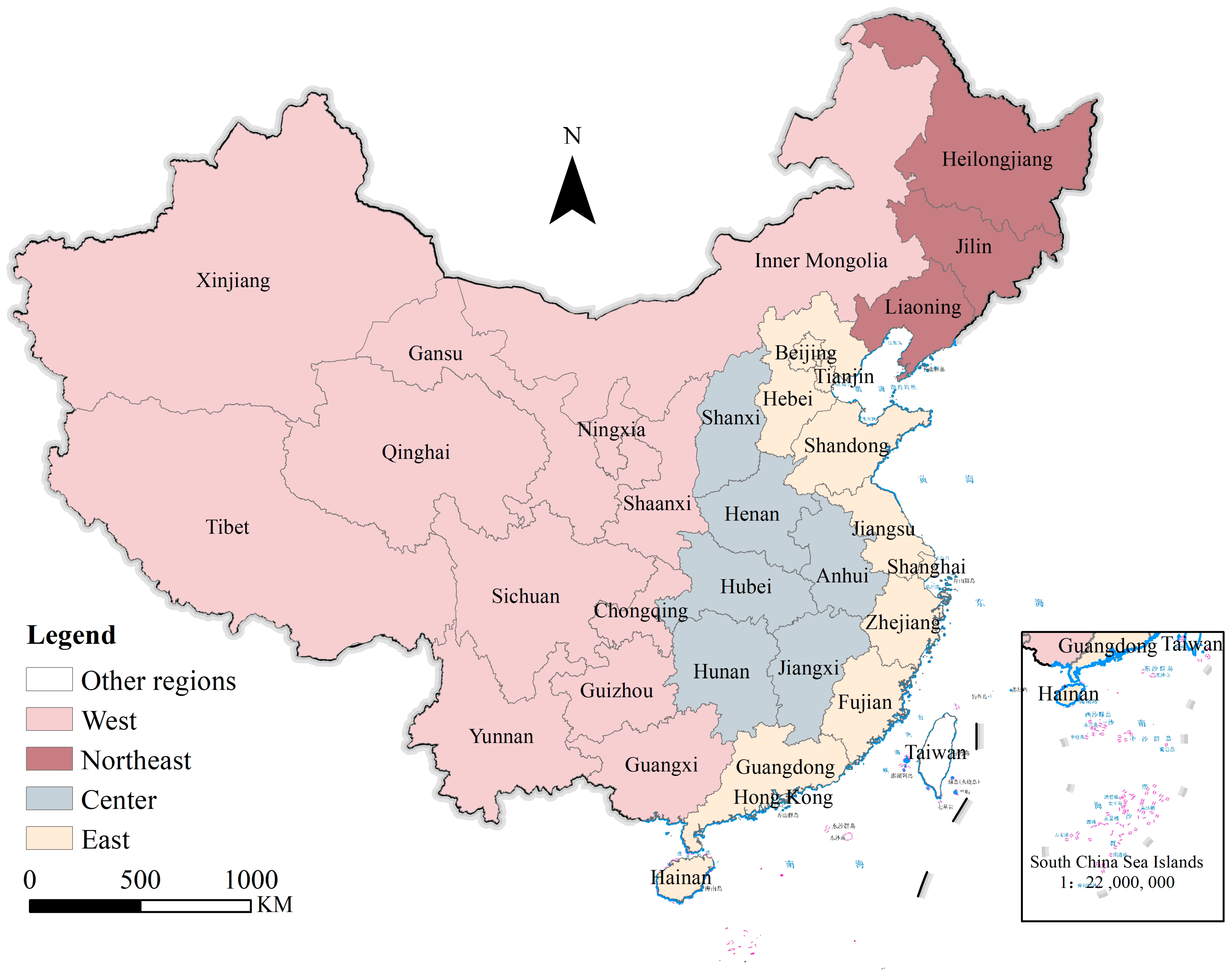
3.4. Research Area and Data Source

The State Council has divided China’s economic regions into four major regions (Figure 2): eastern, central, western, and northeastern. The eastern region includes Beijing, Tianjin, Hebei, Shanghai, Jiangsu, Zhejiang, Fujian, Shandong, Guangdong, and Hainan. The central region includes Shaanxi, Anhui, Jiangxi, Henan, Hubei, and Hunan. The western region includes Inner Mongolia, Guangxi, Chongqing, Sichuan, Guizhou, Yunnan, Xizang, Shaanxi, Qinghai, Ningxia, and Xinjiang. The northeast region includes Liaoning, Jilin, and Heilongjiang. In view of the availability of data, this paper selected 284 cities in the Chinese mainland as the sample. This study divides the 284 cities into eastern cities, central cities, western cities, and northeastern cities based on their provinces. The eastern, central, western, and northeastern regions referred to in this article are the eastern regions of the sample.

The data collected in this study are city-wide data, not city-administered district data. For missing data in individual years, this study used trend functions and interpolation methods to fill in the missing data. In order to eliminate the influence of price factors, the price-related data in the full text have been processed at constant prices, using 1978 prices as the base period. Science and technology expenditures and education expenditures mainly come from the “China Cities Statistical Yearbook” (https://data-cnki-net-443.vpn.bass.org.cn/yearBook/single?id=N2022040095, accessed on 15 June 2022), and social security expenditures and medical and health expenditures mainly come from the CEIC database (https://www.ceicdata.com.cn/zh-hans, accessed on 11 November 2023), and the “China Regional Economic Statistical Yearbook” (2000–2014) (https://data-cnki-net-443.vpn.bass.org.cn/yearBook/single?id=N2015070200, accessed on 8 September 2023). Official-related data comes from CSMAR data (https://data.csmar.com/, accessed on 10 May 2021), People’s Daily Online local leadership database (http://www.people.com.cn/, accessed on 10 March 2021), Zecheng net (http://www.hotelaah.com/liren/index.html, accessed on 9 August 2021) and local government websites.

4. Empirical Analysis

4.1. Spatial Autocorrelation

We used Moran’s I index to test whether there is spatial dependence in the urban EWP. When the Moran’s I index is positive, it indicates a spatial positive correlation between urban EWP. When the sign of Moran’s I index is negative, it indicates a spatial negative correlation between urban EWP, and the larger the absolute value of Moran’s I index, the more obvious the spatial correlation. The calculation method for Moran’s I index is as follows:

$$I=\frac{{\sum }_{\mathrm{i}=1}^{\mathrm{n}}{\sum }_{\mathrm{j}=1}^{\mathrm{n}}{\mathrm{W}}_{\mathrm{i}\mathrm{j}}\left(X_i-\overline{X}\right)\left(X_j-\overline{X}\right)}{S^2{\sum }_{i=1}^n{\sum }_{j=1}^n{W}_{ij}}$$

(5)

In the above equation, $S^2=\frac{1}{n}\sum _{i=1}^n{\left(X_i-\overline{X}\right)}^2,\overline{X}=\frac{1}{n}\sum _{i=1}^n{X}_i,$ where $X_i$ represents the observed EWP of region $i$, and $W_{ij}$ is the spatial weight matrix. The global Moran’s I index calculated based on the geographical adjacency matrix is significantly positive at the 1% and 5% levels (excluding 2018 and 2019), indicating significant spatial clustering characteristics in the ecological welfare performance of Chinese cities.

Local spatial autocorrelation can reveal the connections between cities, and the formula for calculating the local Moran’s I index is as follows:

$$I_i=\frac{x_i-\overline{X}}{S_i^2}\sum _{j=1,j\ne i}^n{W}_{i,j}(x_j-\overline{X})$$

(6)

$$S_i^2=\frac{\sum _{j=1,j\ne i}^n(x_j-\overline{X})}{n-1}-{\overline{X}}^2$$

(7)

$x_i$ representing the urban EWP, $\overline{X}$ being the average urban EWP, and $W_{ij}$ being the spatial weight matrix. If the local spatial Moran’s I index is positive, it indicates that similar samples have clustering effects, while negative values indicate that the clustering of similar samples decreases or even disappears in space. Furthermore, 0 indicates that the samples are randomly distributed and have no spatial correlation. The number of ’high-high’ clustering cities shows a V-shaped change, while the clustering of high low clustering cities shows an inverted V-shaped change. The number of low high and low low city clusters shows an inverted N-shaped change.

4.2. Benchmark Regression Analysis

In order to examine the impact of official promotion incentives on urban EWP, this study adds officials’ education and tenure as control variables. It was found that under the geographical adjacency matrix, inverse distance matrix, and economic geography nested matrix, they all passed the LM test, Wald and LR test, Hausman test, and fixed effect test (

Table 3. The impact of official promotion incentives on urban EWP under three spatial weight matrices.

Variables	Geographic Adjacency Matrix	Inverse Distance Matrix	Economic Geography Nested Matrix
Prom	−0.343 ** (−2.504)	−0.462 *** (−3.354)	−0.426 *** (−3.254)
Mhedu	0.007 ** (2.197)	0.007 ** (2.235)	0.007 ** (2.148)
Mxterm	0.001 (0.750)	0.001 (0.674)	0.001 (0.798)
Finance	0.009 (1.042)	0.019 ** (2.207)	0.022 *** (2.732)
struc2	0.232 *** (3.528)	0.143 ** (2.186)	0.177 *** (2.757)
Tec	0.002 (0.323)	−0.003 (−0.396)	−0.006 (−0.835)
Openess	0.593 ** (2.488)	0.419 * (1.761)	0.461 ** (2.028)
Urbani	−0.000 (−0.012)	0.058 * (1.765)	0.048 (1.501)
Per GDP	−0.086 *** (−3.280)	−0.078 *** (−2.996)	−0.087 *** (−3.472)
W*Prom	−0.115 (−0.564)	0.588 (1.464)	0.156 (0.624)
W*Mhedu	−0.005 (−0.711)	−0.013 (−0.772)	0.001 (0.199)
W*Mxterm	0.003 (1.271)	0.003 (0.522)	−0.002 (−0.619)
W*Finance	0.051 *** (3.711)	0.075 *** (2.641)	0.056 *** (3.603)
W*struc2	−0.320 *** (−2.969)	−0.242 (−1.058)	−0.295 ** (−2.487)
W*Tec	−0.035 *** (−3.521)	−0.030 (−1.415)	−0.019 (−1.582)
W*Openess	−0.367 (−1.029)	0.509 (0.778)	0.388 (0.901)
W*Urbani	0.179 *** (3.690)	−0.153 (−1.451)	−0.082 (−1.210)
W*Per GDP	0.071 * (1.758)	0.157 * (1.790)	0.152 *** (3.204)
$\rho$	0.087 *** (3.746)	0.268 *** (5.319)	0.085 *** (3.218)
R2	0.647	0.645	0.644
N	3692	3692	3692
Log-likelihood	2812.838	2803.106	2798.430
LM spatial lag	21.523 ***	39.547 ***	20.439 ***
robust LM spatial lag	15.002 ***	5.964 **	2.260
LM spatial error	17.317 ***	34.994 ***	19.047 ***
robust LM spatial error	10.796 ***	1.410	0.868
Wald spatial lag	48.684 ***	14.891 *	23.950 ***
LR spatial lag	48.502 ***	14.844 *	23.828 ***
Wald spatial error	51.868 ***	17.626 **	24.893 ***
LR spatial error	51.949 ***	17.914 **	24.802 ***
Hausman	1355.360 ***	71.759 ***	324.745 ***

Notes: t-value in parentheses. *, **, and *** denote statistical significance levels at 10%, 5%, and 1%, respectively.

). Therefore, a two-way fixed effect spatial Durbin model was adopted.

The $\rho$ coefficients are 0.087, 0.268, and 0.085, respectively, and all are significantly positive at 1%, indicating that the urban EWPs of neighboring areas have a significant improvement effect on the local urban EWP. Under the three types of spatial weight matrices, official promotion incentives significantly inhibited the improvement of urban EWP (Table 3). The main effects are −0.343, −0.462, and −0.426, respectively, and are significantly negative at 5%, 1%, and 1%. The spatial spillover effects are −0.115, 0.588, and 0.156, respectively, but they are not significant. Under the incentive of promotion, local officials have the incentive to sacrifice the environment for growth, forming a deformed model in which economic growth replaces social development, thereby inhibiting the improvement of urban EWP. The main reasons are as follows:

Economic growth has the characteristic of strong “visibility”. In the promotion competition, local officials will tilt their limited resources towards explicit “visible public goods”, so that the higher-level government can intuitively inspect and evaluate the promotion of lower-level officials. Public goods such as environmental governance, education, social security, and medical care are not “visible”. Specifically, the environmental protection performance of local officials is difficult to quantify and not intuitive enough. The long-term governance method of “heavy punishment and light rewards” has resulted in low incentives for local government officials to protect the environment [49]. When faced with the dual constraints of GDP assessment and environmental pressure, local officials extend their “polluting hands” to non-assessed and highly spillover items in order to maximize the probability of promotion, thus causing the current pollution phenomenon to worsen. In terms of the provision of public goods such as education and medical care, local officials are driven by the cadre assessment and promotion mechanism with economic performance as a hard indicator. It is difficult for local officials to consider education, which has time lags and spillovers, as a priority. In terms of finance, there must be some slack in investment [50], which results in official promotion incentives having a significant inhibitory effect on urban EWP.

The education level can also reflect the ability of officials to a certain extent. Under the three spatial matrix types, the impact of officials’ education levels on urban EWP is 0.007, and is significantly positive at 5%, indicating that an official’s educational level can increase that official’s attention to environmental protection and welfare improvement, which in turn helps to promote urban EWP. The higher the education of the officials, the more inclined they are to adopt green technologies, learn from domestic and foreign environmental protection experiences to curb environmental pollution, and attach greater importance to welfare improvement, which will help promote urban EWP. This conclusion is consistent with the research results of Wang. The “knowledgeable” cadre team will help increase the proportion of science, education, culture, and health, and their impact on high-quality development is deep-seated and comprehensive [51]. Official tenure has a positive impact on urban EWP, but the effect is not significant.

From the analysis of the control variable results, under the inverse distance matrix and economic geography nested matrix, the level of financial development significantly improves the urban EWP, with effects of 0.019 and 0.022, respectively. The level of financial development in neighboring areas can also significantly improve local EWP, with impact effects of 0.051, 0.075, and 0.056, respectively, all significantly positive at 1%. The impacts of the proportion of the secondary industry on EWP are 0.232, 0.143, and 0.177, respectively, and are significantly positive at the 1%, indicating that the secondary industry has significantly improved the urban EWP, and the economic driving effect is greater than environmental pollution. The impacts of secondary industry in neighboring areas on the urban EWP of the region are −0.320, −0.242, and −0.295, respectively, which are significantly negative at 1% and 5% under the geographical adjacency matrix and economic geography matrix, respectively, indicating that the development of the secondary industry in the region inhibits the EWP of the city in the region, and the environmental pollution effect of neighboring areas on the region is greater than the economic effect. The impact of technological progress on urban EWP is not significant. The impacts of opening up to the outside world on urban EWP are 0.593, 0.419, and 0.461, which are significant at the 5%, 10%, and 5% confidence levels, respectively. The level of openness has no significant impact on the EWP of local cities. Under the inverse distance matrix, the improvement effect of urbanization level on urban EWP is 0.058, which is significant at the 10% confidence level.

The impact of the level of economic development on urban EWP is −0.086, −0.078, and −0.087, respectively, all of which are significant at the 1% confidence level, indicating that the current level of economic development inhibits the improvement of urban EWP. The economic development level of neighboring areas can significantly improve the EWP of local cities, with impact effects of 0.071, 0.157, and 0.152, respectively, which are significant at the 10%, 10%, and 1% confidence levels, respectively.

4.3. Robustness Test

4.3.1. Change the Explanatory Variable: Economic Growth Pressure

Economic growth pressure (Pressure) can be regarded as local officials’ promotion incentives, so this study uses economic growth pressure as a proxy variable for local officials’ promotion incentives. In the context of official promotion tournaments, each local government has the motivation to set higher economic growth targets, and this target setting model will cause local economic development to face growth pressure [52]. When the actual economic growth level of the region deviates from the desirable target, especially when the economic growth target is higher than the actual economic growth rate, the economic growth pressure on local officials will increase significantly. Regarding the measurement method of economic growth pressure, this study draws on the measurement method of Wang, and uses the ratio of the current year’s economic growth target to the previous year’s actual economic growth rate to measure local government economic growth pressure.

As can be seen from

Table 4. The impact of economic growth pressure on urban EWP.

Variable	Adjacency Matrix SDM	Inverse Distance Matrix SDM	Economic Geography Nested Matrix SDM
Pressure	−0.001 * (−1.803)	−0.001 * (−1.922)	−0.001 *** (−2.973)
Mhedu	0.007 ** (2.220)	0.007 ** (2.221)	0.007 ** (2.1525)
Mxterm	0.001 (0.757)	0.001 (0.681)	0.001 (0.805)
Finance	0.009 (1.020)	0.019 ** (2.210)	0.021 *** (2.621)
struc2	0.217 *** (3.314)	0.126 * (1.914)	0.161 ** (2.509)
Tec	0.003 (0.435)	−0.001 (−0.175)	−0.005 (−0.708)
Openess	0.530 ** (2.232)	0.348 (1.465)	0.408 * (1.797)
Urbani	−0.001 (−0.044)	0.061* (1.848)	0.050 (1.551)
Per GDP	−0.044 *** (−3.573)	−0.087 *** (−3.341)	−0.098 *** (−3.939)
W*Pressure	−0.002 (−0.745)	−0.003 (−0.470)	0.001 (0.339)
W*Mhedu	−0.004 (−0.606)	−0.014 (−0.781)	0.001 (0.189)
W*Mxterm	0.004 (1.434)	0.003 (0.530)	−0.002 (−0.623)
W*Finance	0.048 *** (3.499)	0.070 ** (2.463)	0.058 *** (3.719)
W*struc2	−0.324 *** (−2.995)	−0.224 (−0.984)	−0.295 ** (−2.511)
W*Tec	−0.037 *** (−3.622)	−0.030 (−1.439)	−0.021 * (−1.718)
W*Openess	−0.366 (−1.029)	0.556 (0.850)	0.383 (0.890)
W*Urbani	0.183 *** (3.765)	−0.153 (−1.456)	−0.093 (−1.386)
W*Per GDP	0.044 (1.128)	0.148 * (1.720)	0.147 *** (3.121)
N	3692	3692	3692
$\rho$/$\lambda$	0.095 *** (4.102)	0.255 *** (5.026)	0.088 *** (3.333)
R2	0.646	0.644	0.643
Log-likelihood	2808.347	2798.105	2793.377
LM spatial lag	23.182 ***	43.591 ***	21.368 ***
robust LM spatial lag	20.321 ***	12.326 ***	4.496 **
LM spatial error	18.461 ***	36.653 ***	19.339 ***
robust LM spatial error	15.600 ***	5.388 **	2.467
Wald spatial lag	51.451 ***	15.636*	26.398 ***
LR spatial lag	51.388 ***	15.344*	26.323 ***
Wald spatial error	55.009 ***	19.684 **	27.827 ***
LR spatial error	55.162 ***	19.522 **	27.746 ***

Notes: t-value in parentheses. *, **, and *** denote statistical significance levels at 10%, 5%, and 1%, respectively.

, under the three types of spatial weight matrices, economic growth pressure significantly inhibits the improvement of urban EWP, and the impact effects are −0.0008, −0.0010, and −0.0009, respectively. At the level of spatial spillover effects, under the three types of spatial weight matrices, urban economic growth pressure in neighboring areas has no significant impact on the EWP of local cities. When the economic growth pressure is set at a high level, especially when it seriously deviates from the actual economic growth level, greater economic growth pressure will form. In order to cope with the pressure of economic growth, local officials often introduce stronger economic policies to interfere with the normal operations of enterprises and markets, which will distort the expenditure structure, cause environmental pollution, and reduce welfare levels, thereby inhibiting the improvement of urban EWP. This empirical result is consistent with the benchmark test, which once again proves the robustness of the model setting and empirical results.

4.3.2. Lagging Independent Variables: Official Promotion Incentives

Considering that the impact of official promotion incentives on urban EWP may have a lag effect, that is, official promotion incentives in the current year may affect urban EWP in the next year, this study draws on existing research [53] and uses one- and two-period lags for official promotion incentives as core explanatory variables to conduct a robustness test to observe whether its impact on urban EWP changes.

Three types of spatial weight matrices (geographic adjacency matrix, geographical inverse distance matrix, and economic geography nested matrix) were used to lag official promotion incentives by one year, and the economic growth targets from 2007 to 2018 were used to explore the urban EWPs from 2008 to 2019 and the impact of official promotion incentives on urban EWP changes in one lagged period. It can be seen from

Table 5. The impact of one lagged official promotion incentives on urban EWP.

Variables	Adjacency Matrix	Inverse Distance Matrix	Economic Geography Nested Matrix
L1.Promo	−0.141 (−0.991)	−0.273 ** (−2.016)	−0.231 * (−1.692)
Mhedu	0.006 (1.631)	0.006 * (1.710)	0.006 (1.606)
Mxterm	0.001 (0.874)	0.001 (0.722)	0.001 (0.875)
Finance	0.009 (0.919)	0.027 *** (3.108)	0.020 ** (2.289)
struc2	0.218 *** (3.065)	0.137 * (1.927)	0.153 ** (2.213)
Tec	0.002 (0.333)	−0.007 (−1.032)	−0.004 (−0.549)
Openess	0.232 (0.877)	0.106 (0.418)	0.197 (0.783)
Urbani	0.877 (1.359)	0.097 *** (2.579)	0.095 ** (2.565)
Per GDP	−0.098 *** (−3.318)	−0.098 *** (−3.504)	−0.097 *** (−3.466)
W*L.Promo	−0.309 * (−1.807)	—	−0.178 * (−1.874)
W*Mhedu	−0.007 (−1.014)	—	0.001 (0.222)
W*Mxterm	0.004 (1.509)	—	0.000 (0.091)
W*Finance	0.051 *** (3.445)	—	0.062 *** (3.766)
W*struc2	−0.325 *** (−2.784)	—	−0.189 (−1.498)
W*Tec	−0.029 *** (−2.711)	—	−0.017 (−1.326)
W*Openess	−0.627 (−1.547)	—	0.116 (0.242)
W*Urbani	0.200 *** (3.567)	—	−0.099 (−1.208)
W*Per GDP	0.089 (0.089)	—	0.163 *** (3.126)
N	3408	3408	3408
$\rho$/$\lambda$	0.086 *** (3.556)	0.327 *** (6.345)	0.076 *** (2.761)
R2	0.645	0.638	0.642
Log-likelihood	2626.469	2610.106	2612.849
LM spatial lag	16.824 ***	33.886 ***	17.014 ***
robust LM spatial lag	17.007 ***	3.590 *	2.246
LM spatial error	13.058 ***	30.910 ***	15.794 ***
robust LM spatial error	13.241 ***	0.615	1.026
Wald spatial lag	44.082 ***	11.340	20.308 **
LR spatial lag	44.063 ***	11.363	20.228 **
Wald spatial error	47.237 ***	13.168	21.129 **
LR spatial error	47.387 ***	13.246	21.067 **

Notes: t-value in parentheses. *, **, and *** denote statistical significance levels at 10%, 5%, and 1%, respectively.

that official promotion incentives with one lag period have a significant impact on urban EWP. The impact effects under the inverse distance matrix and economic geography nested matrix are −0.273 and −0.231, respectively, and the coefficients are significant. This shows that official promotion incentives in the previous year will inhibit the improvement of urban EWP this year, which is consistent with the benchmark test results. In the spatial spillover effect, under the adjacency matrix and economic geography nested matrix, local official promotion incentives significantly inhibit the improvement of urban EWP in neighboring areas, and the impact effects are −0.309 and −0.178, respectively. The education of officials has a significant promoting effect on the urban EWP of the region under the geographical inverse distance matrix. In the spatial spillover effect, promotion incentives for officials in neighboring areas also have a significant inhibitory effect on the EWP of local cities, indicating that excessive economic growth targets not only inhibit local environmental optimization and welfare improvement, but also affect geographical proximity and the EWP of cities with economic and geographical proximity produces negative spillover effects. The neglect of environmental pollution and welfare improvement caused by the promotion incentives of city officials in neighboring regions will also cause the “imitation effect” of cities in the region, thereby inhibiting the improvement of EWP in cities in the region.

Lagging the economic growth target for two periods, this study selects the economic growth targets from 2007 to 2017 to regress the urban EWP from 2009 to 2019, and observes the impact of the economic growth target lagging for two periods on the urban EWP. According to the results in

Table 6. The impact of official promotion incentives on urban EWP lagged two periods.

Variables	Adjacency Matrix	Inverse Distance Matrix	Economic Geography Nested Matrix
L2.Prom	−0.107 (−0.736)	−0.236 * (−1.690)	−0.225 (−1.611)
Mhedu	0.006 * (1.724)	0.007 * (1.826)	0.006 * (1.710)
Mxterm	0.002 (1.028)	0.002 (0.988)	0.002 (1.138)
Finance	0.009 (0.949)	0.029 *** (3.212)	0.019 ** (2.101)
struc2	0.205 *** (2.634)	0.154 ** (1.982)	0.149 * (1.969)
Tec	0.001 (0.069)	−0.005 (−0.652)	−0.001 (−0.122)
Openess	0.278 (0.963)	0.053 (0.191)	0.181 (0.667)
Urbani	0.101 *** (2.586)	0.137 *** (3.404)	0.141 *** (3.559)
Per GDP	−0.109 *** (−3.319)	−0.116 *** (−3.727)	−0.110 *** (−3.534)
W*L2.Prom	−0.474 ** (−2.057)	—	0.002 (0.006)
W*Mhedu	−0.006 (−0.765)	—	0.008 (1.228)
W*Mxterm	0.006* (1.963)	—	−0.001 (−0.190)
W*Finance	0.057 *** (3.579)	—	0.073 *** (4.136)
W*struc2	−0.358 *** (−2.798)	—	−0.110 (−0.810)
W*Tec	−0.016 (−1.335)	—	−0.017 (−1.174)
W*Openess	−1.169 *** (−2.622)	—	−0.300 (−0.573)
W*Urbani	0.180 *** (2.990)	—	−0.095 (−1.067)
W*Per GDP	0.131 ** (2.557)	—	0.158 *** (2.766)
N	3124	3124	3124
$\rho$/$\lambda$	0.062 ** (2.435)	0.294 *** (5.427)	0.067 ** (2.330)
R2	0.646	0.640	0.644
Log-likelihood	2456.525	2440.501	2446.841
LM spatial lag	10.079 ***	21.972 ***	13.268 ***
robust LM spatial lag	12.771 ***	1.631	2.248
LM spatial error	7.376 ***	20.453 ***	12.112 ***
robust LM spatial error	10.068 ***	0.112	1.092
Wald spatial lag	41.558 ***	14.843*	21.481 **
LR spatial lag	41.526 ***	14.496	21.382 **
Wald spatial error	43.780 ***	15.706*	22.245 ***
LR spatial error	43.790 ***	15.424*	22.185 ***

Notes: t-value in parentheses. *, **, and *** denote statistical significance levels at 10%, 5%, and 1%, respectively.

, among the direct effects, only under the inverse distance matrix are the impacts of official promotion incentives on urban EWP in two lagged periods significant, and the impact effect is −0.236. Among the spatial spillover effects, only under the geographical adjacency matrix do the promotion incentives of officials in neighboring cities lagged by two periods have an inhibitory effect on the EWP of the city in the region, with an impact effect of −0.474. The promotion incentives of city officials in neighboring regions will also inhibit the improvement of urban EWP. The empirical results of official promotion incentives in two lagged periods on urban EWP are similar to those in one lagged period. Compared with official promotion incentives in one lagged period, the impact of official promotion incentives in two lagged periods on urban EWP is smaller. The absolute value is small, indicating that the inhibitory effect of official promotion incentives on urban ecological welfare tends to diminish over time.

4.3.3. Endogeneity Test Based on Instrumental Variable Method

In order to alleviate the endogeneity caused by omitted variables, this study refers to the practice of Yu et al., by constructing an interaction term between the number of cities in provinces (related to individual changes) and the mean of the national economic growth target in the next two years (related to time), as an official promotion incentive instrumental variable [46]. The division of cities belongs to the political level and is decided by the central government. During the study sample period, the number of cities in each province is basically a fixed value and is not affected by the economic variables of each city. If there are more cities in the province where the city is located, the competition for urban GDP will be more intense under the constraints of promotion incentives. It should be noted that due to the impact of the epidemic in 2020, the central government did not set an economic growth target, resulting in a lack of economic growth data for the two years after 2018. Therefore, the sample interval used in the endogeneity test is from 2007 to 2017. In addition, since the number of municipalities and cities is all 1, the data of municipalities in all years are eliminated during the endogeneity test.

From the results in

Table 7. Endogeneity test of official promotion incentives on urban EWP based on two-stage instrumental variables method.

Variables	First Stage	Second Stage
	Promo	EWP
Prom	—	−13.87 *** (3.159)
IV	0.001 ** (0.000)	—
Finance	−0.004 *** (0.001)	−0.078 *** (0.014)
struc2	0.061 *** (0.011)	0.524 ** (0.205)
Tec	−0.006 *** (0.001)	−0.100 *** (0.022)
Openess	0.378 *** (0.056)	4.467 *** (1.227)
Urbani	0.002 (0.006)	0.036 (0.039)
Per GDP	−0.006 * (0.003)	−0.046 * (0.025)
Cons	0.178 *** (0.018)	3.207 *** (0.525)
N	3080	3080
Durbin chi2	84.8619 (p = 0.000)
Wu-Hausman	87.0113 (p = 0.000)

Notes: standard error in parentheses. *, **, and *** denote statistical significance levels at 10%, 5%, and 1%, respectively.

, we can see that both the Durbin and Wu-Hausman test results reject the null hypothesis, indicating that the dependent variable has endogeneity. In the first-stage regression, the F value is 23.22, rejecting the null hypothesis of weak instrumental variables, indicating that the instrumental variables selected in this study are reasonable. In the first-stage regression, instrumental variables have a significant positive impact on official promotion incentives. In the second-stage regression, the impact of official promotion incentives on urban EWP is significantly negative, with an effect of −13.871, which has the same sign as the baseline regression, indicating that after dealing with endogeneity issues, the baseline results are still robust.

4.4. Mechanism of Official Incentive’s Impact on EWP

Promotion is the biggest incentive for officials. The political promotion of local officials is not only closely related to the political cycle but also highly related to the leader’s economic performance and fiscal revenue contribution. Although the central government has included environmental protection and welfare improvement in official evaluation indicators in recent years, local governments still pay more attention to GDP growth due to the “explicit” characteristics of GDP growth and the long-term dependence on GDP promotion paths, as was observed in the government work report [53]. In this context, officials have performance preference incentives and pursue maximizing performance benefits, especially the tendency to maximize explicit performance. Local officials may be more focused on pursuing rapid economic growth during their term of office, investing resources in economic development areas that highlight political performance, and neglecting projects such as environmental protection and public services, resulting in a low preference coefficient for the government’s welfare expenditure structure [39].

The higher the proportion of welfare expenditures, the more it can promote the improvement of urban EWP. The four expenditures of education, social security and employment, medical and health, and science and technology expenditures are closely related to the improvement of EWP [54]. For example, education spending can improve the quality of the labor force and promote economic growth. Expenditure on affordable housing can solve the housing needs of residents, and expenditure on medical and health services can provide more services such as public health and medical service training and improve the level of public welfare. Expenditure on science and technology can improve the level of innovation. All the above four types of expenditures are conducive to improving the performance of urban ecological welfare. When local officials are motivated by promotion, they will reduce the proportion of welfare expenditures. Therefore, official promotion incentives will have an impact on environmental pollution, education investment, social security, and medical and health expenditures, and ultimately inhibit the improvement of EWP. Local officials in other regions adopt imitation strategies in order to gain opportunities for political promotion, so official promotion incentives may lead to a reduction in urban EWP in neighboring regions. In summary, official promotion incentives will affect urban EWP by affecting the proportion of welfare expenditures (fiscal responsiveness), and have spatial spillover effects.

The model that official promotion incentives affect urban EWP by affecting fiscal responsiveness (welfare expenditure structure) is constructed as follows:

$${Response}_{i,t}=\alpha +\beta {Prom}_{i,t}+\gamma X_{i,t}+\theta \sum _{j=1}^N{W}_{ij}{Prom}_{j,t}+\delta \sum _{j=1}^N{W}_{ij}{X}_{j,t}+{\epsilon }_{i,t}$$

(8)

$${EWP}_{i,t}=\alpha +\varnothing {Prom}_{i,t}+\phi {Reponse}_{i,t}+\vartheta X_{i,t}+\sigma \sum _{i\ne j}^N{W_{ij}Prom}_{j,t}+\varrho \sum _{j=1}^N{W}_{ij}{Response}_{j,t}+\tau \sum _{j=1}^N{W}_{ij}{X}_{j,t}+{\epsilon }_{i,t}$$

(9)

${Response}_{i,t}$ represents financial responsiveness, ${Prom}_{i,t}$ represents official promotion incentives, β is the impact of official promotion incentives on financial responsiveness, and θ is the impact of official promotion incentives in neighboring areas on the region. ∅ represents the impact of official promotion incentives on the city’s EWP in the region, φ represents the impact of fiscal responsiveness on the city’s EWP, σ represents the impact of city officials’ promotion incentives in neighboring regions on the city’s EWP, and ρ represents the city’s fiscal response in neighboring regions. Regarding the impact of responsiveness on the EWP of cities in the region, the meanings of other variables are as mentioned above and will not be repeated here.

The steps for choosing which spatial model to choose are as mentioned above and will not be repeated here. It can be seen from

Table 8. Analysis of the mechanism of official promotion incentives affecting urban EWP through fiscal responsiveness.

Variables	Geographic Adjacency SDM		Economic Geography Nested SDM
	Response	EWP	Response	EWP
	(1)	(2)	(3)	(4)
Prom	−0.247 *** (−5.83)	−0.285 ** (−2.071)	−0.211 *** (−5.145)	−0.372 *** (−2.838)
Response	—	0.219 *** (4.096)	—	0.215 *** (4.078)
Mhedu	−0.000 (−0.187)	0.007 ** (2.225)	−0.000 (−0.099)	0.007 ** (2.170)
Mxterm	−0.001 (−1.102)	0.001 (0.806)	−0.001 (−1.185)	0.001 (0.842)
Finance	−0.017 *** (−6.256)	0.013 (1.423)	−0.014 *** (−5.343)	0.025 *** (3.001)
struc2	−0.006 (−0.309)	0.234 *** (3.569)	−0.017 (−0.827)	0.180 *** (2.813)
Tec	−0.002 (−1.141)	0.003 (0.410)	−0.001 (−0.642)	−0.005 (−0.712)
Openess	−0.340 *** (−4.599)	0.644 *** (2.694)	−0.485 *** (−6.791)	0.529 ** (2.312)
Urbani	0.017 * (1.736)	−0.004 (−0.131)	0.020 * (1.961)	0.043 (1.359)
Per GDP	−0.073 *** (−9.003)	−0.071 *** (−2.662)	−0.059 *** (−7.459)	−0.075 *** (−2.962)
W*Prom	0.202 *** (3.225)	−0.162 (−0.799)	0.334 *** (4.252)	0.084 (0.336)
W*Response	—	−0.153 * (−1.667)	—	−0.232 ** (−2.159)
W*Mhedu	0.003 (1.261)	−0.006 (−0.835)	−0.001 (−0.292)	0.001 (0.189)
W*Mxterm	−0.002 ** (−2.201)	0.004 (1.332)	−0.001 (−0.775)	−0.002 (−0.642)
W*Finance	0.011 *** (2.613)	0.048 *** (3.496)	0.004 (0.744)	0.052 *** (3.290)
W*struc2	−0.014 (−0.429)	−0.319 *** (−2.968)	0.036 (0.967)	−0.295 ** (−2.497)
W*Tec	0.003 (1.043)	−0.036 *** (−3.573)	−0.002 (−0.452)	−0.018 (−1.529)
W*Openess	−0.572 *** (−5.125)	−0.335 (−0.914)	−0.601 *** (−4.409)	0.349 (0.792)
W*Urbani	−0.004 (−0.291)	0.182 *** (3.759)	−0.006 *** (−7.459)	−0.075 (−1.109)
W*Per GDP	0.060 *** (4.813)	0.056 (1.380)	0.029* (1.961)	0.128 *** (2.645)
N	3692	3692	3692	3692
$\rho$/$\lambda$	0.266 *** (12.510)	0.090 *** (3.880)	0.213 *** (8.226)	0.089 *** (3.370)
R2	0.691	0.648	0.679	0.646
Log-likelihood	7115.160	2821.392	7057.57	2807.547
LM spatial lag	214.905 ***	22.446 ***	117.525 ***	21.538 ***
robust LM spatial lag	1.148	12.607 ***	2.331 **	0.942
LM spatial error	218.239 ***	18.386 ***	115.512 ***	20.714 ***
robust LM spatial error	4.482 **	8.547 ***	0.318	0.118
Wald spatial lag	86.0653 ***	53.123 ***	57.708	29.575 ***
LR spatial lag	84.942 ***	53.041 ***	57.226	29.463 ***
Wald spatial error	77.058 ***	56.146 ***	56.414 ***	30.053 ***
LR spatial error	76.266 ***	56.320 ***	56.093 ***	29.956 ***
Time effect/double effect	2504.931 ***	3480.833 ***	2504.931 ***	3480.833 ***
Regional effect/double effect	161.957 ***	88.716 ***	161.957 ***	88.716 ***

Note: t-value in parentheses. *, **, and *** denote statistical significance levels at 10%,5%, and 1%, respectively.

that formula (1) is the impact of official promotion incentives on fiscal responsiveness (proportion of welfare expenditures) under the geographical adjacency weight matrix. At the direct effect level, it can be seen that local official promotion incentives significantly inhibit fiscal responsiveness. The impact effect of sex is −0.247. The main reasons are as follows: under the promotion tournament that focuses on GDP assessment, local officials will release “capability signals” to higher-level governments by setting higher economic growth targets, and obtain “tickets for the promotion tournament” by fulfilling the early economic growth targets. Compared with the supply of economic public goods, which can bring the “double benefits” of economic governance performance and fiscal revenue to local governments, the performance of the supply of welfare public goods is often less revealing, and higher-level governments cannot evaluate the capabilities of lower-level governments based on public welfare service projects. Higher-level governments will regularly examine indicators that can be objectively quantified, such as GDP, finance and taxation, investment promotion, etc. In order to improve the “impression score” of superior leaders, local officials will carry out road renovations, city appearance improvements, etc. However, public products with insufficient visibility will not directly affect the evaluation of superior leaders, which will in turn produce visibility bias [55]. To sum up, under the pressure of promotion and limited tenure, local governments have an urgent desire to achieve economic growth goals and will focus their advantageous resources on projects with short economic benefit return cycles and significant marginal contributions to local economic growth goals, resulting in welfare expenditures. Public projects, whose effects are slow and unintuitive, are gradually being squeezed out. At the level of indirect effects, under the two types of spatial weight matrices, promotion incentives for city officials in neighboring regions significantly improve the fiscal responsiveness of cities in the region. The possible reason is that cities in the region and cities in neighboring regions “change tracks” to compete, using the promotion of welfare expenditures to attract more talent to the local area and enhance the competitiveness of urban economic development in the region.

Equation (2) is a spatial Durbin model that adds official promotion incentives and financial responsiveness under the geographical adjacency weight matrix. At the direct effect level, it can be found that official promotion incentives significantly inhibit the improvement of urban EWP, with an impact effect of −0.285, which is significant at the 5% level. Fiscal responsiveness significantly improves urban EWP, with an impact effect of 0.219, which is significant at the 1% level. Combined with the regression results of Equation (1), it can be seen that fiscal responsiveness plays a mediating role in the impact of official promotion incentives on urban EWP. Official promotion incentives inhibit the improvement of fiscal responsiveness, while fiscal responsiveness can improve urban EWP. In order to improve urban EWP, it is necessary to correct official promotion incentives and reduce the inhibitory effect of official promotion incentives on fiscal responsiveness. At the level of spatial spillover effects, it can be found that promotion incentives for city officials in geographically adjacent areas have a negative impact on the EWP of cities in the region, but it is not significant.

The robustness of the results can be tested by transforming the matrix. Equations (3) and (4) are, respectively, the impact of official promotion incentives on fiscal responsiveness under the economic geography nested weight matrix and the impact of official promotion incentives and fiscal responsiveness on urban ecology. It can be seen from (3) that the main effect of official promotion incentives on fiscal responsiveness is −0.211, which is significant at the 1% level, indicating that the higher the official promotion incentives, the lower the fiscal responsiveness. From Equation (4), we can see that official promotion incentives have a significant negative impact on urban EWP. The effect size is −0.372, which is significant at the 1% level, indicating that official promotion incentives significantly inhibit financial responsiveness. Response performance significantly improves urban EWP, with an impact effect of 0.215, which is significant at the 1% level. This shows that official promotion incentives have an impact on urban EWP through financial responsiveness, which is consistent with the test results of Equations (1) and (2). It can be seen from the spatial spillover effect that under the two types of spatial weight matrices, the government fiscal responsiveness of cities in neighboring regions significantly inhibits the improvement of EWP of cities in the region. The impact effects are −0.153 and −0.232, respectively, and are significant at the 10% and 5% levels. The increase in the level of urban welfare expenditures in neighboring areas will intensify the outflow of local brains, thereby hindering local economic development and improving innovation levels, and reducing the EWP of local cities.

4.5. Heterogeneity Analysis

4.5.1. Heterogeneity Analysis Based on East, Middle, West, and Northeast

When exploring the differential impact of official promotion incentives on urban EWP in the eastern, central, western, and northeastern regions, the LM test was used to determine whether to adopt a spatial econometric model. Through the test, it was found that only the northeastern region failed the LM test, and the ordinary OLS regression. On the other hand, the Wald and LR tests were used to determine whether the spatial Durbin model could be used. The test coefficients found that the central and western regions passed the test, while the eastern region failed the Wald and LR tests, so the spatial error model was used.

According to the empirical results (

Table 9. Heterogeneity analysis of official promotion incentives in four major regions on urban EWP.

Variables	Eastern SAR	Central SDM	Western SDM	Northeast OLS
Prom	0.777 ** (2.510)	0.136 (0.390)	−0.450 * (−1.898)	−1.140 *** (−3.953)
Mhedu	0.011 (1.562)	0.003 (0.512)	0.008 (1.199)	−0.003 (−0.263)
Mxterm	0.000 (0.059)	0.003 (1.116)	0.003 (1.290)	0.007 (1.278)
Finance	−0.038 *** (−4.804)	−0.023 (−1.041)	−0.007 (−0.445)	0.073 *** (3.641)
struc2	−0.295 *** (−3.347)	−0.060 (−0.409)	0.247 ** (2.278)	0.538 *** (2.803)
Tec	−0.029 *** (−4.747)	0.026* (1.939)	−0.013 (−1.167)	0.010 (0.445)
Openess	−1.830 *** (−5.670)	−0.114 (−0.206)	0.097 (0.137)	0.026 (0.051)
Urbani	0.285 *** (6.135)	0.012 (0.174)	0.061 (1.224)	−0.012 (−0.106)
Per GDP	−0.013 (−0.675)	−0.080 (−1.437)	−0.086 * (−1.932)	−0.202 *** (−2.870)
W*Prom	—	−0.195 (−0.335)	−0.704 ** (−2.323)	—
W*Mhedu	—	−0.014 (−1.112)	−0.026 ** (−2.035)	—
W*Mxterm	—	0.009 (1.483)	0.008 * (1.900)	—
W*Finance	—	0.061 (1.402)	0.023 (1.000)	—
W*struc2	—	−0.910 *** (−3.730)	−0.478 *** (−2.864)	—
W*Tec	—	−0.057 *** (−2.822)	−0.032 ** (−2.001)	—
W*Openess	—	1.206 (1.198)	−0.948 (−0.812)	—
W*Urbani	—	0.109 (0.954)	0.273 *** (4.055)	—
W*Per GDP	—	0.347 *** (3.658)	0.071 (1.266)	—
N	1118	1040	1092	442
$\rho$/$\lambda$	0.180 *** (4.755)	0.157 *** (3.576)	0.035 (0.948)	—
R2	0.109	0.613	0.655	0.119
Log-likelihood	353.029	875.809	785.336	—
LM spatial lag	0.483	20.530 ***	2.2513	0.699
robust LM spatial lag	5.202 **	8.965 ***	14.763 ***	0.605
LM spatial error	0.007	18.2259 ***	0.9180	1.208
robust LM spatial error	4.725 **	6.661 **	13.429 ***	1.114
Wald spatial lag	12.381	31.619 ***	41.444 ***	—
LR spatial lag	12.132	31.006 ***	40.851 ***	—
Wald spatial error	12.695	32.317 ***	42.514 ***	—
LR spatial error	12.593	32.126 ***	42.168 ***	—
Time effect/double effect	67.706	846.184 ***	845.032 ***	—
Regional effect/double effect	130.327 ***	23.472 **	29.172 ***	—

Notes: t-value in parentheses. *, **, and *** denote statistical significance levels at 10%, 5%, and 1%, respectively.

), official promotion incentives in the eastern region have a positive impact on urban EWP, with an effect of 0.7769, which is significant at the 1% confidence level. Promotion incentives for officials in the central region have a positive impact on urban EWP, but it is not significant. Official promotion incentives in the western and northeastern regions have a significant negative impact on urban EWP, with effects of −0.4502 and −1.1398, respectively, which are significant at the 10% and 1% confidence levels, respectively. At the level of spatial spillover effects, only the central and western parts of the country adopt the spatial Durbin model, and only promotion incentives for urban officials in neighboring regions in the western region have a significant inhibitory effect on the EWP of cities in the region. The effect is −0.7040, and at the 5% confidence level. Promotion incentives for city officials in neighboring regions in the west have distorted the expenditure structure, resulting in urban environmental pollution and a reduction in people’s welfare levels in the region, which in turn has led to a decline in the EWP of cities in the region.

The reason why official promotion incentives in different regions have differential impacts on urban EWP may be that the eastern region has a developed economy and there is less conflict between official promotion incentives and environmental goals. The economic foundation of the eastern region has always held a good advantage among the four major regions. It has a large number of scientific and technological talents and strong scientific research funding. Under the pressure of official promotion, the behavior of local governments will not be alienated. However, the western and northeastern regions have limited space for economic development, and there is an obvious conflict between economic goals and environmental goals. They are facing pressure from economic growth and industrial structure transformation and upgrading. Productive investment, with its short return period and low risk, has become an important force for local governments to promote the rapid rise of the economy. However, technological innovation lacks the support of corresponding infrastructure, funds, human capital, and other factors, making it difficult to promote stable economic growth. On the one hand, the economic development of the western and northeastern regions is relatively backward, and the fiscal gap for public goods expenditure is large. In the short term, the marginal benefit of productive expenditure is much greater than the marginal benefit of welfare expenditure, resulting in the government focusing on productive expenditure and lack of welfare. Expenditures crowd out fiscal expenditures related to innovation activities such as science and technology expenditures, which manifest as official promotion incentives distorting local government fiscal expenditure behavior, leading to a decline in local government welfare levels and a loss of innovation efficiency. On the other hand, the economically underdeveloped western and northeastern regions are unable to attract companies with “clean technologies”. Therefore, local officials take on a large number of polluting enterprises in order to achieve political performance, which will increase the levels of local environmental pollution [56]. Although environmental protection has become one of the areas of inspection for local officials in recent years, local officials’ demands for political performance can cause local officials to ignore environmental protection work in their jurisdictions. In summary, the differences in the economic and social development levels of the four major regions have caused the differential impact of official promotion incentives on urban EWP.

4.5.2. Heterogeneity Analysis Based on Official Age

Economic growth target setting can be regarded as an extrinsic incentive for official promotion, while official age is an intrinsic incentive for official promotion. The vast majority of officials need to be promoted when they are under 55 years old. Therefore, officials aged 53–54 usually face greater internal promotion incentives. So, will the impact of official promotion incentives on urban EWP differ depending on the age of officials?

This study assigns officials a value of 1 when they are 53 and 54 years old, and 0 for other ages. By constructing an interaction term between official age and official promotion incentives, we explore whether there is heterogeneity in the impact of official age on official promotion incentives on urban EWP. It can be found from the results in

Table 10. Heterogeneity test of official age under three spatial weight matrices.

Variables	Geographic Adjacency Matrix	Geographic Inverse Distance Matrix	Economic Geography Nested Matrix
Prom	−0.347 ** (−2.533)	−0.398 *** (−3.390)	−0.429 *** (−3.282)
Age*Prom	−0.061 * (−1.877)	−0.058 * (−1.916)	−0.061 (−1.258)
Mhedu	0.007 ** (2.243)	0.007 ** (2.287)	0.007 ** (2.185)
Mxterm	0.001 (0.685)	0.001 (0.670)	0.001 (0.697)
Finance	0.009 (1.062)	0.027 *** (3.648)	0.022 *** (2.705)
struc2	0.232 *** (3.535)	0.132 ** (2.152)	0.175 *** (2.730)
Tec	0.002 (0.353)	−0.009 (−1.515)	−0.005 (−0.801)
Openess	0.582 ** (2.440)	0.451 ** (2.177)	0.447* (1.967)
Urbani	−0.001 (−0.003)	0.045 (1.538)	0.049 (1.531)
Per GDP	−0.088 *** (−3.337)	−0.076 *** (−3.249)	−0.089 *** (−3.539)
WProm	−0.010 (−0.109)	—	0.084 (0.872)
WAge*Prom	−0.115 (−0.564)	—	0.147 (0.589)
WMhedu	−0.005 (−0.720)	—	0.001 (0.230)
WMxterm	0.003 (1.253)	—	−0.002 (−0.657)
W*Finance	0.050 *** (3.621)	—	0.055 *** (3.538)
W*struc2	−0.327 *** (−3.027)	—	−0.302 ** (−2.544)
W*Tec	−0.035 *** (−3.519)	—	−0.019 (−1.592)
W*Openess	−0.379 (−1.053)	—	0.371 (0.861)
W*Urbani	0.180 *** (3.691)	—	−0.078 (−1.150)
W*Per GDP	3.691 * (1.764)	—	0.150 *** (3.159)
N	3692	3692	3692
$\rho$/$\lambda$	0.088 *** (3.790)	0.293 *** (5.998)	0.084 *** (3.180)
R2	0.647	0.644	0.644
Log-likelihood	2813.668	2796.3213	2799.5736
LM spatial lag	21.421 ***	39.225 ***	20.454 ***
robust LM spatial lag	14.202 ***	5.933 **	2.501
LM spatial error	17.313 ***	34.679 ***	18.966 ***
robust LM spatial error	10.094 ***	1.387	1.013
Wald spatial lag	48.665 ***	14.624	24.471 ***
LR spatial lag	48.570 ***	14.537	24.397 ***
Wald spatial error	51.787 ***	17.353*	25.509 ***
LR spatial error	51.900 ***	17.404*	25.434 ***

Notes: t-value in parentheses. *, **, and *** denote statistical significance levels at 10%, 5%, and 1%, respectively.

that among the direct effects, under the geographical adjacency matrix, official promotion pressure inhibits the improvement of urban EWP, and the interaction term between official age and promotion incentives is negative and significant. This shows that officials aged 53 and 54 will intensify the inhibitory effect of promotion incentives on urban EWP. Under limited terms, 53- and 54-year-old officials have more promotion pressure, so they are more motivated to curb fiscal welfare expenditures and increase the proportion of productive expenditures, which in turn intensifies the inhibitory effect of official promotion incentives on urban EWP. At the level of spatial spillover effects, under the spatial weight matrix of geographical adjacency and economic geography, official promotion incentives do not have a significant impact on the urban EWP. The promotion incentives of 53- and 54-year-old officials in neighboring cities have a significant impact on the local EWP. There is no significant impact on regional urban EWP.

5. Discussion and Conclusions

5.1. Discussion

At the level of the impact of official promotion incentives on urban EWP, there is consistency with the existing research. Some existing studies suggest that although local official promotion incentives promote economic growth, they also bring about local protectionism tendencies, redundant construction, and overcapacity problems, which damage the quality of China’s economic development [57]. The promotion incentives for local officials come from the assessment goals of the central or higher-level government. Although the central government continuously reduces the proportion of economic assessment and increases the weight of environmental protection and other indicators, it has not fundamentally reduced the economic development pressure on local officials [58], which is particularly reflected in the Government Work Report. The report covers a considerable amount of content related to economic development, indicating that economic indicators are still superior to other target settings. The scarce promotion opportunities and shorter tenure make officials more inclined to adopt an extensive development approach that emphasizes economy and neglects environmental protection and welfare, ultimately suppressing the improvement of urban EWP.

5.2. Conclusions

First, through benchmark testing, it was found that official promotion incentives significantly inhibited the improvement of urban EWP. The economic growth pressure was used to measure official promotion incentives, lag official promotion incentives by one and two periods, and construct instrumental variables for robustness testing. It was found that officials’ promotion incentives still significantly inhibit the improvement of urban EWP. Second, using welfare expenditure as a proxy variable for fiscal responsiveness, it was found that official promotion incentives significantly inhibit financial responsiveness, while fiscal responsiveness significantly improves urban EWP. Official promotion incentives affect urban EWP by affecting fiscal responsiveness. Finally, the differential impact of official promotion incentives on urban EWP was analyzed through regional heterogeneity and official age heterogeneity. From the perspective of regional differences, it was found that official promotion incentives in the eastern region significantly improved urban EWP, official promotion incentives in the western and northeastern regions significantly inhibited urban EWP, and official promotion incentives in the central region had no significant effect on urban EWP. From the perspective of official age, local officials aged 53 and 54 who have strong promotion incentives intensify the inhibitory effect of promotion incentives on urban EWP.

5.3. Implications

First, to establish a new development concept and promote high-quality economic development. There is nothing “evil” in the economic growth target itself. The key is the governance concept behind the target setting, which guides local governments to abandon the concept of the one-sided pursuit of economic growth speed. If economic growth targets are set unrealistically and local officials ignore regional factor endowments in order to meet promotion needs, serious consequences will inevitably occur. The setting of local government goals should not focus too much on short-term economic growth performance but should be guided by regional endowments and market rules to avoid local government interference in corporate business decisions.

Second, to promote the development of local government expenditure structures in a more reasonable direction and reduce the negative impact of official promotion incentives on welfare expenditures. On the one hand, this can be achieved by weakening the role of officials in resource allocation or strengthening the supervision of welfare expenditures of local officials, implementing a review system for the resignation of leading cadres, increasing the accountability of cadres with poor environmental governance and welfare performance, and improving the government’s fiscal responsiveness. On the other hand, EWP can be improved by improving government incentive mechanisms and market mechanisms. By innovating local government policy tools, switching from factor-driven to innovation-driven, lowering the GDP target, increasing the proportion of local government assessments on improving the business environment, cultivating the market, protecting the environment, and improving public services, urban EWP can be improved.

Third, to implement differentiated policies in different regions to improve the short-term behavior of local officials in economic and social development. There are large differences in the resource endowments and economic structures of various regions in China. The development tasks and requirements undertaken by each region are also different. Comparable indicators should be formulated according to local conditions and with different emphasis. Each region should give full play to its comparative advantages in the unified national market, to achieve differentiated competition and dislocated development in overall development and mutual collaboration. The eastern region should cultivate world-class advanced manufacturing clusters as soon as possible, continuously improve innovation capabilities, strengthen regional linkage, continue to narrow regional development gaps, and strive to achieve equalization of basic public services. The central region should actively integrate into the national strategy and strengthen the strategic positioning of “one center, four regions”. The western region adheres to innovative development, promotes the conversion of old and new driving forces, expands the level of opening up and exchanges, and promotes the high-quality development of medical and education. The northeast region must proceed towards national defense security, food security, and ecological security, making every effort to break down institutional barriers and improve EWP.

Regarding the impact and mechanism analysis of official promotion incentives on urban EWP, this study mainly set economic growth goals as the main indicator of official incentives through theoretical reasoning. In the future, case analysis methods can be used to discover the main decisive factors of official promotion through in-depth local government research. This article provides empirical evidence for studying the impact of government behavior and has reference significance for other countries facing the same dilemma of balancing the economy, environmental protections, and welfare improvement.

References

1. O’Neill, D.W. The Proximity of Nations to a Socially Sustainable Steady-State Economy. J. Clean. Prod. 2015, 108, 1213–1231. [Google Scholar] [CrossRef]
2. Song, Y.; Mei, D. Sustainable Development of China’s Regions from the Perspective of ecological welfare performance: Analysis Based on GM(1,1) and the Malmquist Index. Env. Dev. Sustain. 2022, 24, 1086–1115. [Google Scholar] [CrossRef]
3. Zhang, C.; Li, J.; Liu, T.; Xu, M.; Wang, H.; Li, X. The Spatiotemporal Evolution and Influencing Factors of the Chinese Cities’ Ecological Welfare Performance. Int. J. Environ. Res. Public Health 2022, 19, 12955. [Google Scholar] [CrossRef] [PubMed]
4. Liu, N.; Wang, Y. Urban Agglomeration Ecological Welfare Performance and Spatial Convergence Research in the Yellow River Basin. Land 2022, 11, 2073. [Google Scholar] [CrossRef]
5. He, S.; Fang, B.; Xie, X. Temporal and Spatial Evolution and Driving Mechanism of Urban Ecological Welfare Performance from the Perspective of High-Quality Development: A Case Study of Jiangsu Province, China. Land 2022, 11, 1607. [Google Scholar] [CrossRef]
6. Song, X.; Tian, Z.; Ding, C.; Liu, C.; Wang, W.; Zhao, R.; Xing, Y. Digital Economy, Environmental Regulation, and Ecological Well-Being Performance: A Provincial Panel Data Analysis from China. Int. J. Environ. Res. Public Health 2022, 19, 11801. [Google Scholar] [CrossRef]
7. Zang, M.; Zhu, D.; Liu, G. Ecological Well-being Performance: Concept, Connotation and Empirical of G20. China Popul. Resour. Environ. 2013, 23, 118–124. (In Chinese) [Google Scholar]
8. Zhu, D.; Zhang, S. Research on Ecological Wellbeing Performance and Its Relationship with Economic Growth China Population. Resour. Environ. 2014, 24, 59–67. (In Chinese) [Google Scholar]
9. Martinez-Vazquez, J.; McNab, R.M. Fiscal Decentralization and Economic Growth. World Dev. 2003, 31, 1597–1616. [Google Scholar] [CrossRef]
10. Long, L.; Wang, X. A study on Shanghai’s ecological well-being performance. China Popul. Resour. Environ. 2017, 27, 84–92. (In Chinese) [Google Scholar]
11. Zhang, S.; Zhu, D. Incorporating “Relative” Ecological Impacts into Human Development Evaluation: Planetary Boundaries–Adjusted HDI. Ecol. Indic. 2022, 137, 108786. [Google Scholar] [CrossRef]
12. Long, L. Evaluation of urban ecological well-being performance of Chinese major cities based on two-stage super-efficiency network SBM Model. China Popul. Resour. Environ. 2019, 29, 1–10. (In Chinese) [Google Scholar]
13. Rochlitz, M.; Kulpina, V.; Remington, T.; Yakovlev, A. Performance Incentives and Economic Growth: Regional Officials in Russia and China. Eurasian Geogr. Econ. 2015, 56, 421–445. [Google Scholar] [CrossRef]
14. Zhou, L. The Incentive and Cooperation of Government Officials in the Political Tournaments: An Interpretation of the Prolonged Local Protectionism and Duplicative Investments in China. Econ. Res. J. 2004, 50, 33–40. (In Chinese) [Google Scholar]
15. Zhang, J.; Gao, Y. Term Limits and Rotation of Chinese Governors: Do They Matter to Economic Growth? J. Asia Pac. Econ. 2007, 53, 91–103. (In Chinese) [Google Scholar] [CrossRef]
16. Zheng, S.; Kahn, M.E.; Sun, W.; Luo, D. Incentives for China’s Urban Mayors to Mitigate Pollution Externalities: The Role of the Central Government and Public Environmentalism. Reg. Sci. Urban Econ. 2014, 47, 61–71. [Google Scholar] [CrossRef]
17. Zhao, L.; Shao, K.; Ye, J. The Impact of Fiscal Decentralization on Environmental Pollution and the Transmission Mechanism Based on Promotion Incentive Perspective. Env. Sci. Pollut. Res. 2022, 29, 86634–86650. [Google Scholar] [CrossRef] [PubMed]
18. Zhou, B.; Liu, S.; Liu, L. Local Officials and Regional Tourism Economies. Tour. Anal. 2023, 28, 387–402. [Google Scholar] [CrossRef]
19. Tian, Z.; Tian, Y. Political Incentives, Party Congress, and Pollution Cycle: Empirical Evidence from China. Envir. Dev. Econ. 2021, 26, 188–204. [Google Scholar] [CrossRef]
20. Cole, D.W.; Cole, R.; Gaydos, S.J.; Gray, J.; Hyland, G.; Jacques, M.L.; Powell-Dunford, N.; Sawhney, C.; Au, W.W. Aquaculture: Environmental, Toxicological, and Health Issues. Int. J. Hyg. Environ. Health 2009, 212, 369–377. [Google Scholar] [CrossRef]
21. Yu, Y.; Yang, X.; Li, K. Effects of the Terms and Characteristics of Cadres on Environmental Pollution: Evidence from 230 Cities in China. J. Environ. Manag. 2019, 232, 179–187. [Google Scholar] [CrossRef]
22. Chen, T.; Wang, Y.; Luo, X.; Rao, Y.; Hua, L. Inter-Provincial Inequality of Public Health Services in China: The Perspective of Local Officials’ Behavior. Int. J. Equity Health 2018, 17, 108. [Google Scholar] [CrossRef] [PubMed]
23. Ihori, T.; Yang, C.C. Interregional Tax Competition and Intraregional Political Competition: The Optimal Provision of Public Goods under Representative Democracy. J. Urban. Econ. 2009, 66, 210–217. [Google Scholar] [CrossRef]
24. Xie, X.; Zhang, M.; Zhong, C. Temporal and Spatial Variations in China’s Government-Official-Appointment System and Local Water-Environment Pollution. Sustainability 2022, 14, 8868. [Google Scholar] [CrossRef]
25. Zhang, Y.; Zhang, T.; Zeng, Y.; Yu, C.; Zheng, S. The Rising and Heterogeneous Demand for Urban Green Space by Chinese Urban Residents: Evidence from Beijing. J. Clean. Prod. 2021, 313, 127781. [Google Scholar] [CrossRef]
26. Wang, S.; Sun, X.; Song, M. Environmental Regulation, Resource Misallocation, and Ecological Efficiency. Emerg. Mark. Financ. Trade 2021, 57, 410–429. [Google Scholar] [CrossRef]
27. Wang, S.; Zhao, D.; Chen, H. Government Corruption, Resource Misallocation, and Ecological Efficiency. Energy Econ. 2020, 85, 104573. [Google Scholar] [CrossRef]
28. Charnes, A.W.; Cooper, W.W.; Rhodes, E.L. Measuring The Efficiency of Decision Making Units. Eur. J. Oper. Res. 1979, 2, 429–444. [Google Scholar] [CrossRef]
29. Tone, K. A Slacks-Based Measure of Efficiency in Data Envelopment Analysis. Eur. J. Oper. Res. 2001, 130, 498–509. [Google Scholar] [CrossRef]
30. Tone, K. A Slacks-Based Measure of Super-Efficiency in Data Envelopment Analysis. Eur. J. Oper. Res. 2002, 143, 32–41. [Google Scholar] [CrossRef]
31. Kahn, M.E.; Li, P.; Zhao, D. Water Pollution Progress at Borders: The Role of Changes in China’s Political Promotion Incentives. Am. Econ. J. Econ. Policy 2015, 7, 223–242. [Google Scholar] [CrossRef]
32. Huang, L.; Wang, Z.; Wang, X. The Impact and Mechanism of Local Economic Growth Target on Foreign Direct Investment. Int. Econ. Trade Res. 2021, 37, 51–66. [Google Scholar]
33. Eaton, S.; Kostka, G. Authoritarian Environmentalism Undermined? Local Leaders’ Time Horizons and Environmental Policy Implementation in China. China Q. 2014, 218, 359–380. [Google Scholar] [CrossRef]
34. Wang, X.; Huang, L. Local Economic Growth Target Management—A Triple-factor Framework of Theoretical Construction and Empirical Test. Econ. Theory Bus. Manag. 2019, 345, 30–44. (In Chinese) [Google Scholar]
35. Zhang, Y.; Mao, W.; Zhang, B. Distortion of Government Behaviour under Target Constraints: Economic Growth Target and Urban Sprawl in China. Cities 2022, 131, 104009. [Google Scholar] [CrossRef]
36. Li, X.; Liu, C.; Weng, X.; Zhou, L.-A. Target Setting in Tournaments: Theory and Evidence from China. Econ. J. 2019, 129, 2888–2915. (In Chinese) [Google Scholar] [CrossRef]
37. Edin, M. State Capacity and Local Agent Control in China: CCP Cadre Management from a Township Perspective. China Q. 2003, 173, 35–52. [Google Scholar] [CrossRef]
38. Ma, L. Performance Feedback, Government Goal-Setting And Aspiration Level Adaptation: Evidence From Chinese Provinces. Public Adm. 2016, 94, 452–471. [Google Scholar] [CrossRef]
39. Que, W.; Zhang, Y.; Schulze, G. Is Public Spending Behavior Important for Chinese Official Promotion? Evidence from City-Level. China Econ. Rev. 2019, 54, 403–417. [Google Scholar] [CrossRef]
40. Yin, H.; Yang, L. Research into the Responsiveness of Local Government Finance to Resident Preference. Soc. Sci. China 2014, 221, 96–115+206. (In Chinese) [Google Scholar]
41. López, R.; Galinato, G.I.; Islam, A. Fiscal Spending and the Environment: Theory and Empirics. J. Environ. Econ. Manag. 2011, 62, 180–198. [Google Scholar] [CrossRef]
42. Mina, A.; Lahr, H.; Hughes, A. The Demand and Supply of External Finance for Innovative Firms. Ind. Corp. Chang. 2013, 22, 869–901. [Google Scholar] [CrossRef]
43. Fang, M.; Chan, C.K.; Yao, X. Managing Air Quality in a Rapidly Developing Nation: China. Atmos. Environ. 2009, 43, 79–86. [Google Scholar] [CrossRef]
44. Shahidullah, A.K.M.; Choudhury, M.-U.-I.; Emdad Haque, C. Ecosystem Changes and Community Wellbeing: Social-Ecological Innovations in Enhancing Resilience of Wetlands Communities in Bangladesh. Local Environ. 2020, 25, 967–984. [Google Scholar] [CrossRef]
45. Dean, J.M.; Lovely, M.E.; Wang, H. Are Foreign Investors Attracted to Weak Environmental Regulations? Evaluating the Evidence from China. J. Dev. Econ. 2009, 90, 1–13. [Google Scholar] [CrossRef]
46. Guan, X.; Wei, H.; Lu, S.; Dai, Q.; Su, H. Assessment on the Urbanization Strategy in China: Achievements, Challenges and Reflections. Habitat Int. 2018, 71, 97–109. [Google Scholar] [CrossRef]
47. Dietz, T.; Rosa, E.A.; York, R. Environmentally Efficient Well-Being: Is There a Kuznets Curve? Appl. Geogr. 2012, 32, 21–28. [Google Scholar] [CrossRef]
48. Li, X.; Zhao, C.; Cao, J. Official Turnover and Sustainable Development in China. J. Chin. Polit. Sci. 2023. [Google Scholar] [CrossRef]
49. Luo, W.; Qin, S. China’s Local Political Turnover in the Twenty-First Century. J. Chin. Polit. Sci. 2021, 26, 651–674. [Google Scholar] [CrossRef]
50. Jia, J.; Guo, Q.; Zhang, J. Fiscal Decentralization and Local Expenditure Policy in China. China Econ. Rev. 2014, 28, 107–122. [Google Scholar] [CrossRef]
51. Wang, X.; Zhang, L.; Xu, X. What Determines Local Fiscal Expenditure Propensity: On the Jurisdiction Leaders Perspective. Comp. Econ. Soc. Syst. 2013, 26, 157–167+180. [Google Scholar]
52. Zhang, C.; Liu, T.; Li, J.; Xu, M.; Li, X.; Wang, H. Economic Growth Target, Government Expenditure Behavior, and Cities’ Ecological Efficiency—Evidence from 284 Cities in China. Land 2023, 12, 182. [Google Scholar] [CrossRef]
53. Zhang, J.; Wang, J.; Yang, X.; Ren, S.; Ran, Q.; Hao, Y. Does Local Government Competition Aggravate Haze Pollution? A New Perspective of Factor Market Distortion. Socio-Econ. Plan. Sci. 2021, 76, 100959. [Google Scholar] [CrossRef]
54. Chen, H.; Singh, B.; Aru, W.S. Relationship between Government Expenditure and Economic Growth: Evidence from Vanuatu. J. Asia Pac. Econ. 2022, 27, 640–659. [Google Scholar] [CrossRef]
55. Keefer, P. Democracy, Public Expenditures, and the Poor: Understanding Political Incentives for Providing Public Services. World Bank Res. Obs. 2005, 20, 1–27. [Google Scholar] [CrossRef]
56. Jiang, S.-S.; Li, J.-M. Do Political Promotion Incentive and Fiscal Incentive of Local Governments Matter for the Marine Environmental Pollution? Evidence from China’s Coastal Areas. Mar. Policy 2021, 128, 104505. [Google Scholar] [CrossRef]
57. Yu, Y.; Li, K.; Duan, S.; Song, C. Economic Growth and Environmental Pollution in China: New Evidence from Government Work Reports. Energy Econ. 2023, 124, 106803. [Google Scholar] [CrossRef]
58. Wu, H.; Yang, J.; Yang, Q. The Pressure of Economic Growth and the Issuance of Urban Investment Bonds: Based on Panel Data from 2005 to 2011 in China. J. Asian Econ. 2021, 76, 101341. [Google Scholar] [CrossRef]
Figure 1. Research framework.
Sustainability 16 03085 g001
Figure 2. Division of four regions in China. Note: the map is drawn according to the Standard Map Service Website of the Ministry of natural resources (map review No. GS (2020) 4630).
Sustainability 16 03085 g002