Abstract
From 2008 to 2021, this study analyzed the spatial correlation characteristics between provincial transportation carbon emission intensity and explored ways to reduce transportation carbon emissions. This study used the modified gravity model, social network analysis (SNA) method, and temporal exponential random graph model (TERGM) to analyze the spatial correlation network evolution characteristics and driving mechanism of China’s transportation carbon emission intensity. This study found that China’s transportation carbon emission intensity and spatial correlation network have unbalanced characteristics. The spatial correlation network of transportation carbon emission intensity revealed that Shanghai, Beijing, Tianjin, Guangdong, Fujian, and other provinces were at the center of the network, with significant intermediary effects. The spatial correlation of transportation carbon emission intensity was divided into four functional plates: “two-way spillover”, “net benefit”, “broker”, and “net spillover”. The “net benefit” plate was mainly located in developed regions, and the “net spillover” plate was primarily located in underdeveloped regions. Endogenous structural and exogenous mechanism variables were the main factors affecting the evolution of the spatial correlation network of provincial transportation carbon emission intensity.
1. Introduction
Low-carbon development is a topic that has gained much attention both locally and globally. Data show that in 2009, China’s carbon dioxide emissions surpassed those of the United States, making it the largest carbon-emitting country worldwide [1]. To address this issue, the Chinese government has developed a series of emission reduction plans. In 2009, during the Copenhagen Climate Conference, China committed to reducing its carbon emissions per unit of GDP by 40% to 45% compared to the 2005 levels by 2020. In 2015, China made another commitment to peak its carbon emissions around 2030 and strive for a 60% to 65% reduction in carbon emissions per unit of GDP compared to 2005 levels by 2030 [2,3]. In September 2020, at the United Nations’ General Assembly, China pledged to achieve carbon peaking by 2030 and strive for carbon neutrality by 2060. In September 2021, China reiterated its “dual-carbon” goals at the United Nations’ General Assembly. This commitment has received significant international attention and positive evaluations from the global community.
Transportation is a crucial sector of the economy and plays a leading role [4,5]. However, it also contributes to almost 25% of global carbon emissions [6,7]. This is a major concern as it poses significant threats to human health and the environment [8]. In recognition of this, the Chinese government has included “ecological civilization construction” in the “Five-sphere Integrated Plan” since the 18th National Congress. It has implemented several policies to reduce carbon emissions in transportation, such as the “Green Transportation 14th Five-Year Development Plan” [9]. Despite these efforts, developing low-carbon transportation in China needs to be accelerated to address the severe situation. China is currently undergoing rapid development in “triple integration” (industrialization, urbanization, motorization) but has yet to undergo fundamental transformations in technological levels and energy structures. Therefore, it is foreseeable that transportation carbon emissions will continue to deteriorate in the future [10,11,12].
Transportation carbon emissions are unique as they are produced by mobile sources. The inter-provincial flow of cars, trains, and airplanes will generate transportation carbon emissions for the local area. As a result, there are spatial correlations among provinces in terms of transportation carbon emissions. A correlation network has formed due to the improved transportation infrastructure and increasing complexity of transportation flows, such as people and goods moving between regions. However, this phenomenon has limited our ability to develop targeted emission reduction measures due to significant provincial differences in transportation scales across China. An in-depth analysis of transportation carbon emission intensity, rather than just total quantity, is more reliable in understanding provincial scale factors and formulating effective emission reduction strategies. Therefore, it is crucial to understand and identify the spatial correlation characteristics and driving mechanisms of transportation carbon emission intensity to promote carbon reduction in transportation and develop regional collaborative emission reduction strategies [13].
This paper focuses on transportation carbon emission intensity. It analyzes inter-provincial transportation carbon emission data from 2008 to 2021 to construct a spatial correlation network. Social network analysis (SNA) is used to conduct a multi-faceted analysis of the spatial correlation network characteristics [14,15]. The temporal exponential random graph model (TERGM) is also incorporated to reveal the driving mechanisms of the network structure’s evolution from both static cross-sections and dynamic correlation changes [16]. The goal is to provide a reference basis for formulating differentiated policies for carbon reduction in transportation and building cross-regional collaborative governance mechanisms. The contributions of this paper are two-fold: (1) empirical analysis from the perspective of transportation carbon emission intensity, which excludes the scale factors of various provinces; and (2) the first application of the TERGM to analyze the driving mechanisms of the spatial correlation network of transportation carbon emission intensity. The TERGM can integrate endogenous structural variables and exogenous mechanism variables into a unified framework for driving mechanism analysis, and provides a detailed study of the dynamic change mechanisms of the network.
The remainder of this paper is organized as follows. Section 2 provides a review of the relevant literature. Section 3 introduces and explains the research method and data source. Section 4 presents empirical research and analysis of the results. Finally, Section 5 offers conclusions and policy recommendations.
2. Literature Review
Many researchers have conducted extensive research on transportation carbon emissions and analyzed various aspects such as estimating transportation carbon emissions at different scales [17,18,19], predicting transportation carbon emissions [20], assessing the potential for transportation carbon reduction [21], identifying factors influencing transportation carbon emissions [22], and simulating policies and scenarios for transportation emission reduction [23]. When analyzing the spatial structure of transportation carbon emissions, scholars primarily focus on two aspects: the spatiotemporal characteristics of transportation carbon emissions, and the network characteristics and influencing factors of transportation carbon emissions.
2.1. The Spatiotemporal Characteristics of Transportation Carbon Emissions
In recent years, scholars have conducted extensive research on transportation carbon emissions. They have realized the importance of adopting a spatial perspective to explore regional carbon reduction. This research mainly focuses on the spatiotemporal distribution patterns of transportation carbon emissions at different scales and their spatial heterogeneity. For instance, Koutrakis et al. [24] studied the spatial distribution of transportation carbon emissions in the federal regions of Brazil using Moran’s index. Shu et al. [25] used a multiple linear regression model and spatial decomposition methods to classify urban transportation carbon emissions into regional categories. Huang et al. [26] analyzed the spatial flow and characteristics of transportation carbon emissions caused by tourism in Jiangsu Province by collecting transportation data from self-driving tourism. Li et al. [27] analyzed the spatial pattern evolution of transportation carbon emissions in 341 cities in China, revealing significant regional variations at the urban level. Yuan et al. [28] quantitatively calculated the transportation carbon emission intensity of Chinese provinces based on the IPCC method and analyzed its spatial characteristics. Fu et al. [29] analyzed the spatial distribution characteristics of carbon emission efficiency in the transportation industry in the Yangtze Economic Belt using Moran’s index.
2.2. The Network Characteristics and Influencing Factors of Transportation Carbon Emissions
Scholars have been using complex network techniques to analyze the global spatial patterns of transportation carbon emissions. To construct carbon emission spatial networks, different methods have been employed. Although some scholars have used regional input–output models [30], this method takes a considerable amount of time to compile and analyze, which affects the research’s timeliness. Therefore, many scholars have resorted to using gravity models to construct transportation carbon emission spatial correlation networks [31], which have proven to be a better solution for the timeliness issue and opened up new ways of conducting research. On this basis, many scholars have identified critical regions in the spatial correlation network of transportation carbon emissions by analyzing the network’s overall characteristics, individual characteristics, spatial clustering, etc. [32].
Furthermore, some scholars have explored the factors that influence carbon emission spatial correlation networks. They have used panel models to analyze the impact of network structural characteristics, population size, energy structure, and other attribute variables on global carbon emissions [33]. They have also used a Qualified Allocation Plan (QAP) to examine the formation mechanisms of carbon emission spatial correlation networks [34,35]. However, these models have limitations in examining the impact effects of attribute and relational variables separately. The formation of carbon emission spatial correlation relationships is often simultaneously influenced by endogenous structural variables, exogenous, and other multidimensional attribute variables and relationship variables. To overcome these limitations, some scholars have introduced the Exponential Random Graph Model (ERGM) to study carbon emission spatial correlation networks [36]. The ERGM is considered one of the most effective tools in social network analysis. It comprehensively analyzes various related factors’ roles in forming spatial correlation networks [37,38,39]. The ERGM estimates and tests the endogenous and exogenous mechanisms of network relationship formation. It is based on the dependence between variables and tests whether the convergence of multiple local spatial networks can generate global network structural characteristics [40,41,42]. This research provides valuable insights for exploring the formation mechanisms of transportation carbon emission spatial correlation networks.
2.3. Literature Review
Transportation carbon emissions have been extensively studied by researchers worldwide. According to the research conclusions of previous scholars, transportation carbon emission reduction faces huge challenges because the location of transportation carbon emissions is not fixed. The effect of relying solely on each province to implement transportation carbon emission reduction policies is not ideal. Therefore, targeted transportation carbon emission reduction policies should be formulated based on the characteristics of its spatial correlation network, and regional coordinated transportation carbon emission reduction across provinces and departments should be carried out [31,32].
Most studies have focused on the spatiotemporal characteristics, spatial correlations, and driving mechanisms of transportation carbon emissions in general and not specifically on transportation carbon emission intensity. Studying the spatial correlation network and the factors that drive transportation carbon emission intensity can help eliminate differences caused by the varying scales of each province. This can lead to more accurate research results and provide effective suggestions for reducing transportation carbon emissions. In addition, previous studies on the factors influencing spatial correlation networks have often used QAP methods or the ERGM. QAP methods only consider the influence of exogenous “correlated data” such as population, industrial structure, and technological level differences. However, in the case of spatial correlation networks of transportation carbon emissions, the primary influencing factors are endogenous structural variables, exogenous attributes, and relationship variables. Ignoring such factors can lead to inaccurate estimation results. The traditional ERGM is a static network analysis method that can only reveal the network formation mechanism at a specific time. It is unsuitable for analyzing the dynamic mechanisms of network changes. The TERGM proposed by Hanneke et al. can integrate endogenous structural and exogenous mechanism variables into a unified framework for analyzing influencing factors and facilitates the study of dynamic changes in the network [43]. Studying the network’s dynamic change mechanism can help us understand the impact of various driving factors on the network, providing a useful reference for nationwide coordinated transportation carbon emissions reduction.
After analyzing numerous papers related to the low-carbon field, we have noticed that several policy recommendations have been made for reducing carbon emissions in the transportation field. On the other hand, the building field has made remarkable progress in low-carbon development, specifically in reducing carbon emissions in building operations. This progress can provide useful insights for implementing more effective transportation carbon emission reduction policies [44,45].
3. Methodology and Data Source
3.1. Transportation Carbon Emission Intensity Measurement
Transportation carbon emission intensity is a measure of the amount of carbon emissions produced for each unit of transportation gross production. It helps to understand the relationship between the transportation industry and the carbon emissions it produces. This measure is an indirect way to consider the impact of the transportation industry on economic development [28]. It is calculated as follows:
where represents the transportation carbon emission intensity of province i; represents the transportation carbon emissions of province i; and represents the gross transportation production value of province i.
3.2. Spatial Correlation Strength
Spatial correlation network construction and strength measurement are key components of Social Network Analysis (SNA). To create a spatial correlation network of provincial transportation carbon emission intensity, each province is represented as a node in the network, and the spatial correlation of each province’s transportation carbon emission intensity is represented by a connection. The construction of the network is mainly carried out using the VAR model [46] and the gravity model [47,48,49]. However, the VAR model is too sensitive to the selection of lag order and cannot accurately depict the structural characteristics of the network. Therefore, this paper chooses the gravity model to quantify the spatial correlation relationship of transportation carbon emission intensity, which requires a modification of the basic formula [50,51]. The modified gravity model is presented below:
where is the correlation strength of transportation carbon emission intensity between province i and province j; is the end-of-year population of province i; is the transportation carbon emission intensity of province i; is the deflated GDP of province i with 2000 as the base period; is the contribution ratio of province i in the correlation of transportation carbon emission intensity between province i and province j; and the ratio of the geographical distance to the difference in per capita GDP represents the influence of economic and geographical distance factors, where represents the straight-line distance between province i and province j.
We can calculate the spatial correlation matrix of a province’s transportation carbon emission strength using Formula (2). To create a threshold sparse network, we take the average value of the correlation intensity data in each row of the matrix (excluding the highest and lowest values). We assign a value of 1 to any data that are more elevated than the threshold, and a value of 0 to any data below the threshold. This gives us a directed 0–1 network matrix.
3.3. Social Network Analysis
Social Network Analysis (SNA) is a sociological method used to analyze interpersonal social relationship networks. It has been applied in various fields, including energy [52], tourism [53], and economics [54]. In recent years, scholars have also used SNA to study the spatial correlation of carbon emissions in the environmental field [55,56]. This paper draws inspiration from those studies and uses UCINET 6.0 to analyze the correlation network characteristics of interprovincial transportation carbon emission intensity. It examines the network’s structure and attribute characteristics through network density, centrality, and block model. The specific description is as follows.
3.3.1. Network Density Analysis
The degree of connection strength between transportation carbon emission intensity among provinces is reflected by network density. The specific formula is as follows:
where D is the correlation network density of provincial transportation carbon emission intensity. The closer the value is to 1, the closer the connection between provincial transportation carbon emission intensity; N is the number of provinces; and L is the correlation quantity of transportation carbon emission intensity between provinces.
3.3.2. Individual Network Analysis
Centrality is a concept in network analysis that refers to the importance of a node in a network. There are three types of centrality: degree centrality, closeness centrality, and betweenness centrality.
Degree centrality is further divided into two types in directed graphs: outdegree centrality and indegree centrality. Outdegree centrality measures the number of connections from a node to other nodes, while indegree centrality measures the number of connections to a node from other nodes.
Closeness centrality is a measure of how close a node is to all other nodes in the network. However, it is rarely used in practice due to the high requirements for network completeness [32].
Betweenness centrality measures a node’s control over connecting other nodes in the network. It calculates the number of shortest paths that pass through a node and is often used to identify critical nodes in a network. The calculation formula for betweenness centrality is as follows:
where BC(i) represents the betweenness centrality of province i in the transportation carbon emission intensity network; represents the total number of connections involving the transportation carbon emission intensity between province j and province k; and represents the number of shortest paths between province j and province k that pass through province I, where j ≠ k ≠ i, and j < k.
3.3.3. Block Model Analysis
The block model is a technique used to classify network nodes and identify their specific roles based on the characteristics of the relationship network [57]. It involves comparing the expected ratio of internal relationships with the actual ratio of internal relationships. Each node can be classified into four plates: “two-way spillover”, “net benefit”, “broker”, and “net spillover”. Among them, the “two-way spillover” plate means that members of this plate have more spillover relationships to other plates and within the plate; the “net benefit” plate means that the number of relationships that this plate receives from other plates is much greater than the number of relationships that it has spilled out of the plate; the “broker” plate means that members of this plate both receive and send out more relationships to other plates, playing the role of intermediaries and bridges in the network; and the “net spillover” plate means that members of this plate have significantly more spillover relationships with other plate members than they receive from different plates.
3.4. Temporal Exponential Random Graph Model
3.4.1. Construction of the TERGM
The TERGM is a statistical method used to analyze networks. It has many advantages, such as being able to analyze the endogenous mechanism of network evolution, include time trends, and analyze the dynamic evolution mechanism of the network from a more comprehensive perspective. It has been widely used in recent years to explore the driving mechanisms of spatial correlation networks [58]. This paper constructs the TERGM of the spatial correlation network driving mechanisms of transportation carbon emission intensity based on the assumption that the time interval is one year.
where and refer to the spatial correlation network of provincial transportation carbon emission intensity in periods t and t − 1, respectively; is the normalization constant; is the coefficient vector of the influencing factors of the observation network; and the subscripts s and r refer to the network sending object and receiving object, respectively. Among them, edges, mutual, gwidegree, gwesp, and gwdsp are network structure effects; stability and variability are time-dependent items; POP, GDP, and GT are actor–attribute effects; and dist represents dyadic predictors.
3.4.2. Variable Description in TERGM
- (1)
- Network structure effects
The self-organization of a network shapes its unique spatial structural characteristics [59]. In this context, we can describe the endogenous structure of the network through various measures such as edges, mutual, gwidegree, gwesp, and gwdsp. The edges measure is similar to the intercept in a classic regression model under non-networking. The mutual measure describes the tendency of provinces to form mutual relationships. For instance, if a spatial correlation network relationship of transportation carbon emission intensity is issued in one direction in the current period, the possibility of the other party returning a reciprocal relationship in the next period is higher. Gwidegree reflects the tendency of province i to receive transportation carbon emission intensity relationships sent by multiple other provinces. Gwesp, also known as edge-wise shared partners, examines the possibility that two nodes in the network form a spatial correlation network of transportation carbon emission intensity through a third-party province. Lastly, gwdsp reflects whether there is a “multi-element 2-path” structure in the spatial correlation network of transportation carbon emission intensity relationships between province i and province j. In simpler terms, a 2-path structure in a directed network refers to two nodes transmitting relationships through one or more intermediate nodes, and these intermediate nodes also send or receive relationships from other nodes [60].
- (2)
- Time-dependent items
Stability emphasizes the degree of stability in the spatial correlation network pattern from period t to t + 1. Variability refers to whether there is a trend of change or disappearance in the connectivity status of the spatial correlation network over time.
- (3)
- Actor–attribute effects
Regarding the spatial correlation network of transportation carbon emission intensity, this study is based on existing research settings and data and includes key factors that may affect the province’s transportation carbon emission intensity such as provincial population size (POP), GDP, and green technology level (GT). Given that the spatial correlation network relationship of transportation carbon emission intensity is usually a directed behavior formed by both participants, this paper will further conduct an empirical analysis on the impact of “sending objects” and “receiving objects”.
- (4)
- Dyadic predictor
To examine how geographical distance impacts the correlation between provinces, this paper has developed a spatial adjacency matrix. This matrix is based on the distance between 31 different provinces in the country, with a value of 1 indicating adjacency and 0 indicating non-adjacency. The matrix is used as an exogenous network within the TERGM. As geographical distance affects the socioeconomic connections between provinces, provinces closer to proximity are more likely to establish or maintain a spatial correlation network relationship in transportation carbon emission intensity.
3.5. Data Sources
For this research, 31 provinces in China have been selected as the research objects due to the lack of data on Hong Kong, Macau, and Taiwan. The transportation carbon emission data from 2008 to 2021 used in this paper has been obtained from the Multi-Scale Emission Inventory Reanalysis and Data Sharing Platform of the MEIC Team of Tsinghua University (http://meicmodel.org.cn/, accessed on 5 January 2024). The rest of the data have been extracted from the “China Statistical Yearbook”. To account for the lack of notable statistics on the gross transportation production value data and the small share of the warehousing, postal, and telecommunications industries, the gross production value data of “transportation, warehousing, postal, and telecommunications industries” has been used as a data indicator. The GDP deflator has been used to convert the data into constant prices in 2000 to eliminate the impact of price factors on GDP. The green patent data have been obtained from the China Innovation Patent Research Database. The geographical distance between different provinces has been calculated through ArcGIS 10.8 software and reflected by the Euclidean distance between provincial capital cities.
4. Results and Discussion
4.1. Transportation Carbon Emission Intensity Measurement Results
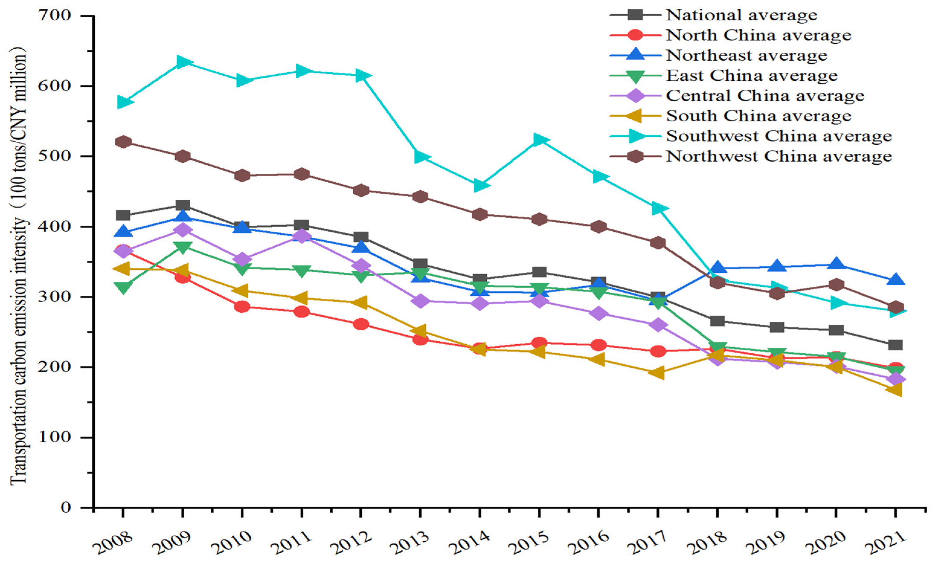
Based on Formula (1), this paper measured the transportation carbon emission intensity of 31 provinces in China from 2008 to 2021. This study drew an evolution trend map for the entire country, as well as for Northeast China, North China, East China, Central China, South China, Southwest China, and Northwest China. Among them, based on the division of topography and climate, Northeast includes Liaoning, Jilin, and Heilongjiang; North China includes Beijing, Tianjin, Hebei, Shanxi, and Inner Mongolia; East China includes Shanghai, Jiangsu, Zhejiang, Shandong, and Anhui; Central China including Hunan, Hubei, Henan, and Jiangxi; South China includes Guangdong, Guangxi, Hainan, and Fujian; Southwest China includes Sichuan, Chongqing, Guizhou, Yunnan, and Tibet; and Northwest China includes Shaanxi, Gansu, Xinjiang, Qinghai, and Ningxia. Figure 1 shows that the national average transportation carbon emission intensity decreased from 416 tons/CNY million in 2008 to 336 tons/CNY million in 2015, and then to 232 tons/CNY million in 2021. This suggests a year-over-year decrease in transportation carbon emission intensity in China and a positive trend of transportation carbon emission reduction.
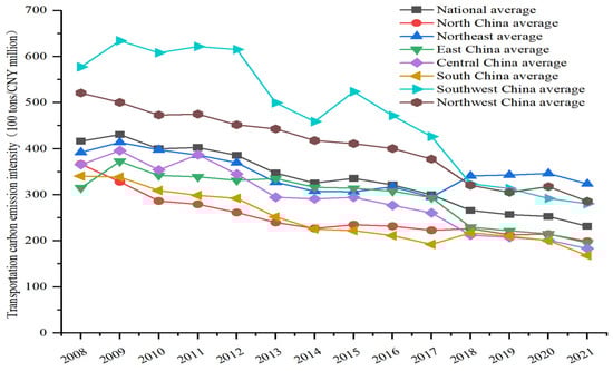
Figure 1.
Time evolution trend of transportation carbon emission intensity in Chinese provinces from 2008 to 2021.
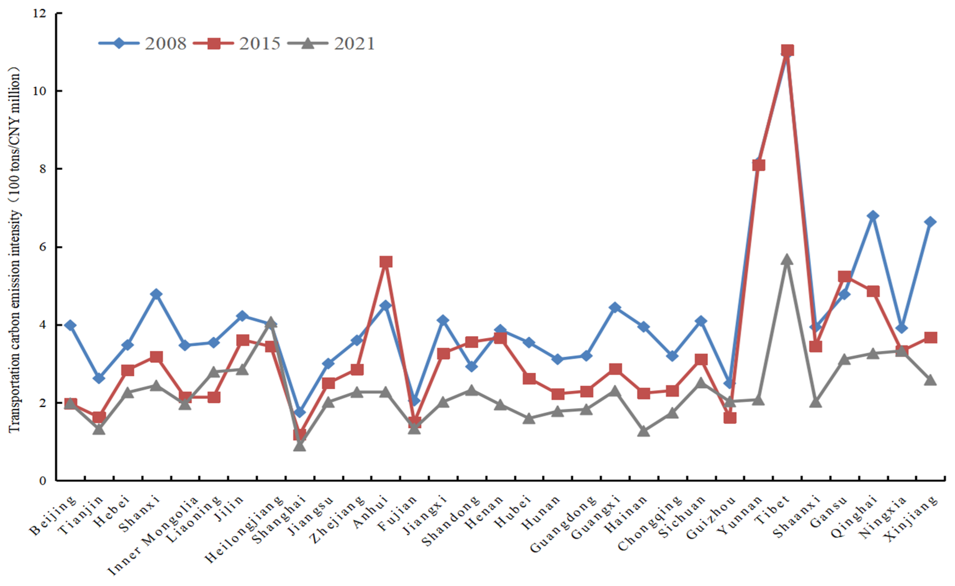
Looking at the seven main regions, Northeast China had an average transportation carbon emission intensity of 348 tons/CNY million, Southwest China had an average transportation carbon emission intensity of 475 tons/CNY million, and Northwest China had an average transportation carbon emission intensity of 407 tons/CNY million, which is significantly higher than the national average. The remaining four regions exhibit a decreasing gradient from South China to North China, then Central China and East China, with average values lower than the national average. Transportation carbon emission intensity in all regions, except Northeast China, showed a downward trend from 2017. At the inter-provincial level, to better analyze the characteristics of transportation carbon emission intensity in each province, the research period of 14 years was evenly decomposed. As a result, 2008, 2015, and 2021 were chosen as the three characteristic years to examine the characteristics of transportation carbon emission intensity before, during, and after the sample period. Figure 2 shows that, except for the three provinces of Liaoning, Heilongjiang, and Guizhou, which had significantly higher transportation carbon emission intensity in 2021 than in 2015, the transportation carbon emission intensity of other provinces showed a downward trend. Additionally, the inter-provincial differences were relatively noticeable.
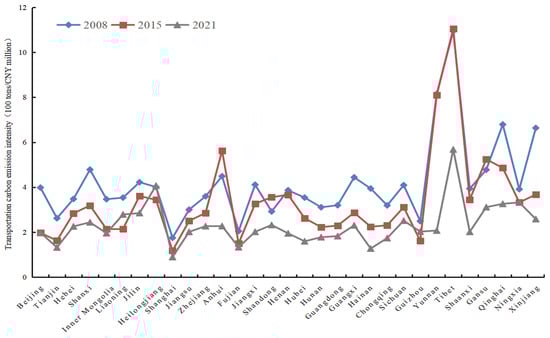
Figure 2.
Time evolution trend of transportation carbon emission intensity in Chinese provinces in 2008, 2015 and 2021.
This paper measures the Gini coefficient of national transportation carbon emission intensity and shows that the transportation carbon emission intensity of various provinces in the country has significant uneven characteristics. However, this difference has shown a gradual decreasing trend over the study period, and the balance of spatial distribution has improved. This suggests that there may be convergence properties. This study further uses ArcGIS to draw the spatial distribution map of national transportation carbon emission intensity in 2008, 2015, and 2021. Figure 3, Figure 4 and Figure 5 show that the transportation carbon emission intensity of China displays an overall trend of “low in the East and high in the West”. The intensity of transportation carbon emission in Northeast China is generally higher than in East and South China. Although each province’s overall transportation carbon emission intensity has gradually declined over time, the three Northeastern provinces have shown an upward trend. This may be due to the cold weather in the northeast, which makes it challenging to apply new energy vehicles, and the applicability of electric cars is weak. Additionally, there are issues such as slowing economic growth and brain drain in the northeast, leading to a lower gross transportation production value. Furthermore, the western provinces of Xinjiang, Tibet, Qinghai, Yunnan, and other provinces have higher transportation carbon emission intensity all year round. This is because Tibet and Qinghai are plateaus with inconvenient roads. Moreover, these provinces need more supporting infrastructure such as charging piles, and new energy vehicles’ popularization is difficult. However, the decrease in transportation carbon emission intensity in the Western region is much more significant than in other regions over time. This indicates that China’s Western development policy has strengthened exchanges and cooperation between the Eastern and Western regions. The economic and technological levels of the Western region have increased, and significant progress has been made in transportation energy-saving and emission reduction technologies, transportation organization efficiency, and transportation industry upgrading. The number of provinces in high-value regions with transportation carbon emission intensity dropped from four in 2008 to one in 2021, and the number of provinces in the low-value regions dropped from nine in 2008 to five in 2021, once again confirming that spatial distribution gradually converges.
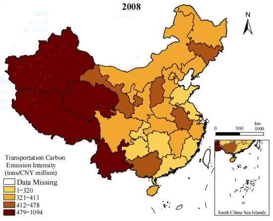
Figure 3.
Spatial evolution pattern of transportation carbon emission intensity in China (2008).
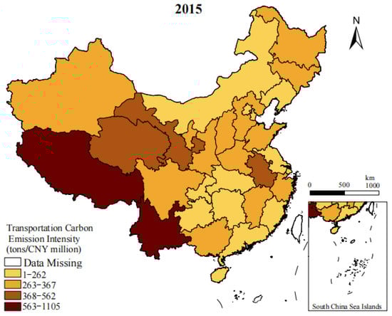
Figure 4.
Spatial evolution pattern of transportation carbon emission intensity in China (2015).
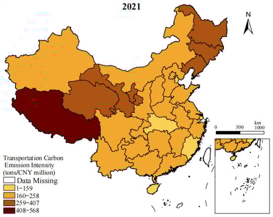
Figure 5.
Spatial evolution pattern of transportation carbon emission intensity in China (2021).
4.2. Spatial Network Structural Characteristics of Transportation Carbon Emission Intensity
4.2.1. Network Density Characteristics
This study calculated the spatial network correlation number and density of transportation carbon emission intensity. The results revealed that between 2008 and 2021, the network correlation number of transportation carbon emission intensity showed a trend of fluctuating evolution, with values of 249 in 2008, 265 in 2015, and 261 in 2021. The network density also indicated a trend of fluctuation, with values of 0.2677 in 2008, 0.2849 in 2015, and 0.2816 in 2021. These values demonstrated a certain degree of stability. However, when looking at the correlation strength, the national average transportation carbon emission intensity correlation strength was 35.81 in 2008, 195.62 in 2015, and 495.19 in 2021. This indicates that China’s spatial correlation network of transportation carbon emission intensity is becoming more and more closely connected.
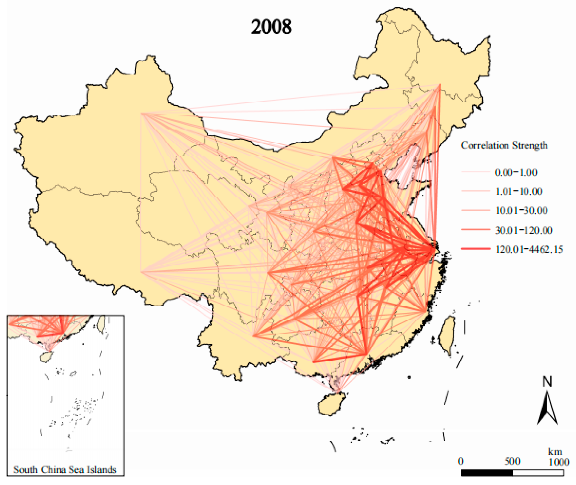
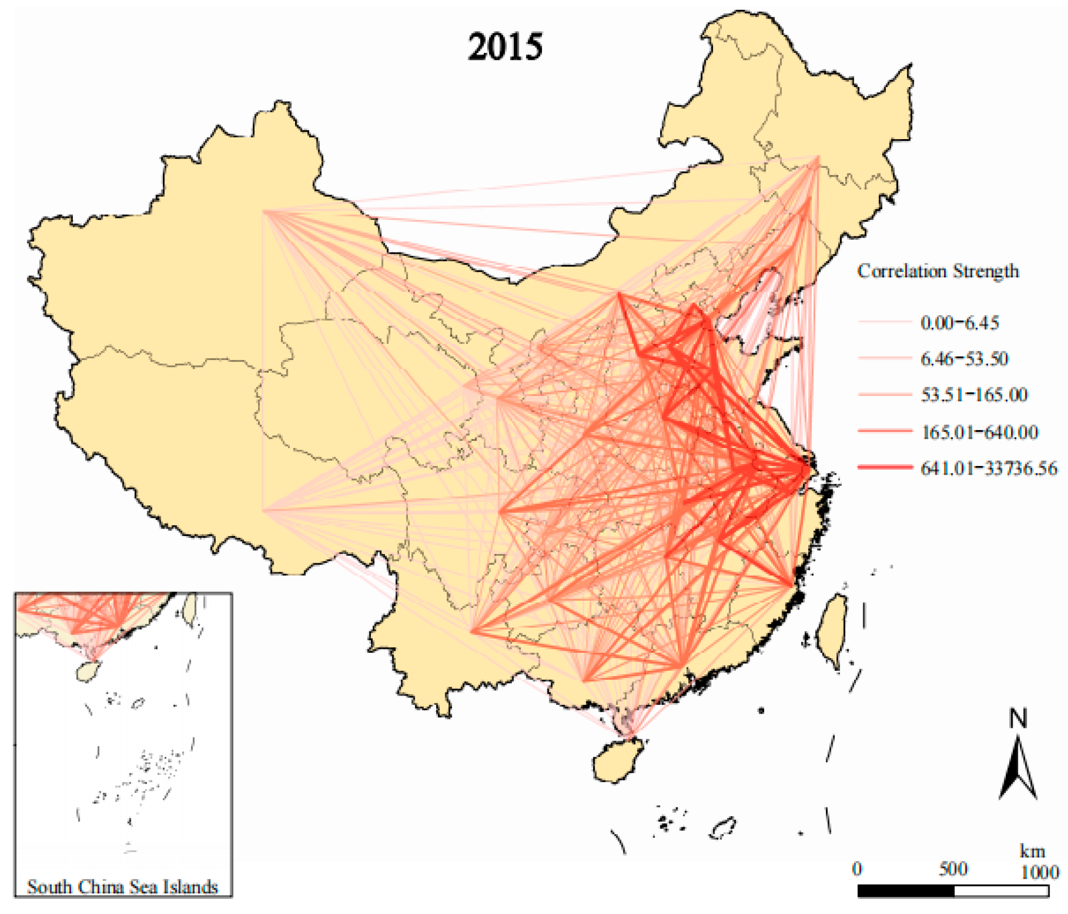
This paper aimed to visually depict the spatial characteristics of China’s transportation carbon emission intensity’s spatial correlation network. This study visualized the spatial network correlation strength of transportation carbon emission intensity in Chinese provinces in 2008, 2015, and 2021 (Figure 6, Figure 7 and Figure 8). This study’s findings indicate that the spatial correlation network of transportation carbon emission intensity in Chinese provinces shows the characteristics of uneven interweaving and high complexity, with prominent spatial non-equilibrium and a spatial distribution pattern of “dense in the East and sparse in the West”.

Figure 6.
Spatial correlation network of transportation carbon emission intensity in China (2008).
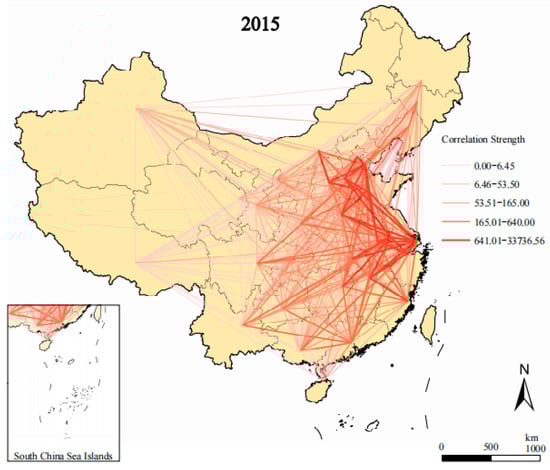
Figure 7.
Spatial correlation network of transportation carbon emission intensity in China (2015).
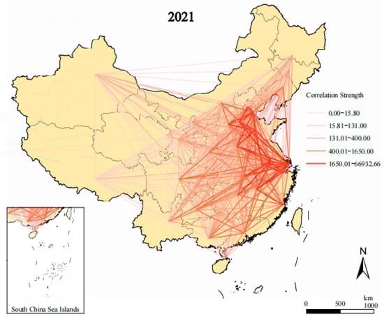
Figure 8.
Spatial correlation network of transportation carbon emission intensity in China (2021).
During the study period, none of the provinces were isolated in the network structure. Furthermore, the transportation carbon emission intensity of the provinces had a cross-regional correlation with non-adjacent provinces, exceeding the limitation of geographical proximity. The spatial correlation network of provincial transportation carbon emission intensity continues to strengthen, forming a spatial structure with Beijing–Tianjin–Hebei, Yangtze River Delta, and Pearl River Delta as the center, and radiating to the surrounding provinces.
The spatial correlation strength of transportation carbon emission intensity in the Eastern and central regions is significantly higher than in the Western and Northeastern regions. The reason for this is that the transportation infrastructure in the Central and Eastern regions is relatively sound, accelerating the flow of innovative resources such as talents, knowledge, and technology, causing the spatial correlation strength of transportation carbon emission intensity in each region to continue to increase.
Although the correlation strength of transportation carbon emission intensity between the Western region and other provinces across the country grows yearly, the overall correlation strength with other provinces is still relatively small. Therefore, it is necessary to further deepen cross-regional low-carbon transportation collaboration, optimize the transportation industry’s spatial layout planning in different regions, and gradually establish and improve transportation carbon emission reduction collaborative governance mechanisms.
4.2.2. Individual Network Characteristics
To analyze the influence and status of various provinces in the spatial correlation network of transportation carbon emission intensity, we calculated each province’s degree of centrality and betweenness centrality. Table 1 shows the calculation results. Concerning degree centrality, the average indegree values for 2008, 2015, and 2021 were 8.032, 8.548, and 8.419, respectively, and the average outdegree values for each year were the same. On the other hand, the average betweenness centrality values for 2008, 2015, and 2021 were 15.457, 20.581, and 18.419, respectively. Notably, the indegree and outdegree of each province during the three-time spans remained stable, with a slight variation. Betweenness centrality exhibited a trend of initially increasing and then decreasing in 13 provinces, including Beijing. At the same time, five provinces, including Guangdong provinces, exhibited a trend of first reducing and then rising. The remaining 13 provinces remained stable. Moreover, compared to 2015, the average indegree, outdegree, and betweenness centrality decreased in 2021. This may be due to the significant impact on the transportation industry caused by the 2019 epidemic, which reduced the correlation between transportation carbon emission intensity among provinces.

Table 1.
Centrality analysis results of inter-provincial transportation carbon emission correlation network in 2008, 2015 and 2021.
The comparison of the average indegree and outdegree in various Chinese provinces over many years showed that Beijing, Jiangsu, Zhejiang, Tianjin, Shandong, and some other provinces had higher indegrees than the average in most years. These provinces are among the top-ranked ones with solid economic strength, human resources, and a relatively complete transportation network. They are also subject to higher “spatial spillover effects” from other provinces in the transportation carbon emission intensity spatial correlation network. These provinces have long-term strategic emerging industries and close cooperation with surrounding provinces. On the other hand, provinces such as Hainan, Tibet, Ningxia, Heilongjiang, Yunnan, Qinghai, and Xinjiang have lower indegrees. They are ranked lower, indicating they need closer correlation with transportation carbon emission intensity among other provinces. These provinces are on the edge of the correlation network and need to catch up in economic development and improve their transportation and logistics network. More cooperation and exchanges with other provinces are required to promote low-carbon undertakings. The outdegree is the opposite of indegree. Unlike developed provinces such as Shanghai, Guangdong, and Fujian, which have higher outdegrees and indegrees, most other provinces with high outdegrees are those with low indegrees.
From the comparison of the average betweenness centrality, Shanghai, Beijing, Tianjin, Guangdong, Fujian, and some other provinces have relatively high betweenness centrality. This indicates that these provinces serve as “intermediaries” and “bridges” in the transportation carbon emission intensity spatial correlation network. They are essential in supporting and controlling cooperation with other provinces in low-carbon transportation development and have a crucial position in the correlation network. It is worth noting that the betweenness centrality of Qinghai, Tibet, Hainan, Ningxia, and Xinjiang provinces is 0, indicating that they are in a “passive” and “marginalized” position in the spatial correlation network of transportation carbon emission intensity. The role of controlling and influencing network correlation has yet to be exerted. Therefore, the spatial correlation of China’s transportation carbon emission intensity has unbalanced characteristics among various node provinces and mainly depends on economically developed central provinces such as Shanghai, Beijing, Tianjin, Guangdong, and Fujian.
4.2.3. Block Model Characteristics
The CONCOR method is a technique that examines the regional differences and spatial correlation network of China’s transportation carbon emission intensity. It uses 2 as the maximum segmentation depth and 0.2 as the convergence standard. With this method, each province in China can be divided into four plates, as shown in Table 2.
Table 2.
Inter-provincial transportation carbon emission intensity block model results in 2008, 2015 and 2021.
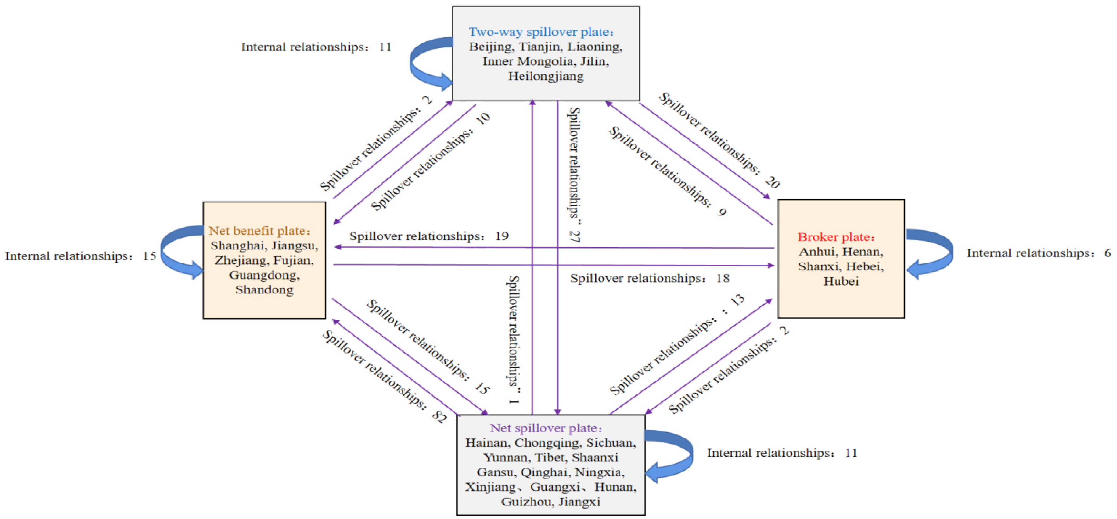
China’s transportation carbon emission intensity is divided into four plates based on a three-year division. The provinces within each plate show little change, and the four plates play the same role each year. For instance, in 2021, each plate was analyzed using the block model, and the results are shown in Figure 9.
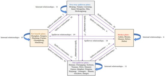
Figure 9.
Block model analysis in 2021.
Plate I is a “two-way spillover plate” comprising six provinces: Beijing, Tianjin, Inner Mongolia, Liaoning, Heilongjiang, and Jilin. The spillover relationship number of this plate is 31, and the receiving relationship number is 38. The expected internal relationship ratio is 16.67%, but the actual internal relationship ratio is 26.19%. Plate I has many spatial correlations internally and externally, making it a “two-way spillover plate”.
Plate II includes six provinces: Guangdong, Jiangsu, Fujian, Zhejiang, Shanghai, and Shandong. The spillover relationship number of this plate is 35, and the receiving relationship number is 111. The internal relationship number of the plate is only 15. The expected internal relationship ratio is 16.67%. but the actual internal relationship ratio is 30.00%. Plate II is classified as a “net benefit plate” because the number of receiving relationships is much greater than the number of spillover relationships, indicating that the spatial spillover effect of this plate is small, and the economies of the provinces within the plate are relatively developed, which has a siphon effect on surrounding provinces.
The members of Plate III include the five provinces of Hebei, Anhui, Henan, Shanxi, and Hubei. The number of spillover relationships in this plate is 30, and the number of receiving relationships is 51. The expected internal relationship ratio is 13.33%, and the actual internal relationship ratio is 16.67%. Plate III plays a “connecting link” in the spatial correlation network and geographical location of China’s transportation carbon emission intensity. Therefore, it is classified as the “broker plate”.
Plate IV includes a total of 14 provinces, including Jiangxi and Hunan. The spillover relationship number of this plate is 122, and the receiving relationship number is 18. The expected internal relationship ratio is 43.33%, and the actual internal relationship ratio is 8.27%. Plate IV has a significant spatial spillover effect, and because the economy is relatively backward, it not only transports transportation energy to the outside world but also loses labor. Hence, Plate IV should be classified as a “net spillover plate”.
In summary, the spatial correlation of China’s transportation carbon emission intensity mainly occurs between plates, and the correlation between provinces within plates needs to be strengthened. There is heterogeneity in the role of each plate in the network, with the “net benefit” plates primarily located in developed regions and the “net spillover” plate primarily located in less developed regions.
4.3. Driving Mechanism
4.3.1. Baseline Regression Analysis
ThIS study used the TERGM to determine the parameters of the spatial correlation network of transportation carbon emission intensity in Chinese provinces from 2008 to 2021. The findings are presented in Table 3. Model 1 is the standard model, and Models 2, 3, and 4 were developed by adding mutual variables, three structural variables, and two-time variables in sequence. Model 4 includes both exogenous mechanism variables and endogenous structural variables. The results show that the addition of endogenous structural variables has a significant impact on the network. However, the impact of exogenous mechanism variables on the overall network has been reduced. The endogenous structural variables have a more substantial effect on the changes in the overall network. Therefore, the regression analysis results of Model 4 were used to analyze the impact of various indicators on the spatial correlation network of provincial transportation carbon emission intensity.
Table 3.
Empirical results of TERGM, a spatial correlation network of transportation carbon emission intensity in Chinese provinces.
Our study on the correlation network of transportation carbon emission intensity in Chinese provinces, based on Model 4, takes into account the impact of both endogenous structural and exogenous mechanism variables. The following is a detailed analysis:
- (1)
- Network structure effects
The spatial correlation network of provincial transportation carbon emission intensity is not random, as indicated by the edge coefficient of −4.10, which passes the significance test. Similarly, the mutual coefficient of 3.67, which also passes the significance test, shows that transportation carbon emission intensity in different provinces promotes the formation of the spatial correlation network. The gwidegree coefficient, which is negative and passes the significance test, suggests that the convergence characteristics of China’s transportation carbon emission intensity correlation network are not conducive to the formation and maintenance of dependence relationships, but the preference for dependence is more obvious. Additionally, the gwdsp coefficient of −0.24, which is significant, indicates that the transmission of the transportation carbon emission intensity relationship between the two provinces in the country is relatively limited by relying on multiple intermediate provinces, and gwdsp is not conducive to the formation of network relationships. Finally, Models 3 and 4 demonstrate that the gwesp coefficient is significantly positive, suggesting that it is more likely for two provinces to form a spatial correlation network of transportation carbon emission intensity through the third province.
- (2)
- Time-dependent items
The stability coefficient of China’s transportation carbon emission intensity is 1.67, and it passes the significance test. This indicates that there is a relatively stable relationship in the spatial correlation of China’s transportation carbon emission intensity, which is gradually strengthening over time. The coefficient of variability is negative and small, which means that the spatial correlation network of China’s transportation carbon emission intensity has a suppressed mutual influence during the process of changing over time. However, its performance is insignificant.
- (3)
- Actor–attribute effects
The analysis of Model 4 in Table 3 indicates that the estimated coefficients for population size, GDP, and green technology level of the sending effect have all passed the significance test. The coefficient of population size is positive, while the coefficients of GDP and green technology level are negative. This suggests that provinces with larger populations, lower GDP, and lower levels of green technology have a higher tendency to send spatial correlation network relationships of transportation carbon emission intensity. The reason may be that the population tends to gather in developed provinces and cities, and less developed provinces strive to seek exchanges and cooperation with developed provinces and cities in low-carbon related fields to acquire emission reduction technical knowledge and reduce the transportation carbon emission intensity in the region. Guizhou, Qinghai, Tibet, Gansu, Xinjiang, and other provinces have a very high outdegree, which belongs to the “net spillover” plate and has more outward connections—ranking higher among provinces across the country.
Regarding the receiver effect, the estimated coefficients of population size, GDP, and green technology level are all significant. The coefficients of GDP and green technology level are significantly positive, indicating that the more developed the economy, the higher the level of green technology in provinces, and the higher the probability of receiving the spatial correlation network relationship of transportation carbon emission intensity. The population size level coefficient is negative, indicating that the larger the regional population, the lower the tendency of receiving the spatial correlation network relationship of transportation carbon emission intensity. As shown in the centrality analysis above, although cities such as Shanghai, Beijing, and Tianjin have small populations, their indegrees are very high, and they receive many relationships from other provinces.
- (4)
- Dyadic predictor
The positive and significant coefficient of geographical distance suggests that the adjacent provinces have a higher spatial correlation of transportation carbon emission intensity. The coordination among the adjacent or similar provinces is less complicated, and the level of transportation interconnection is higher. This can effectively promote the formation of a spatial correlation network of transportation carbon emission intensity, which establishes a mechanism for coordinating cross-regional transportation carbon emission reduction efforts.
The spatial correlation network of China’s transportation carbon emission intensity is influenced by both an endogenous structure and exogenous variables. As more variables such as mutual, gwidegree, gwesp, gwdsp, stability, and variability are added, the impact of exogenous variables on the network decreases. Examining only one dimension of factors to explore the formation of the spatial correlation network of transportation carbon emission intensity may lead to deviations. Therefore, it is important to analyze and discuss the joint action of endogenous and exogenous mechanism factors to better understand the formation and evolution of the network.
4.3.2. Robustness Test
This study aims to test the reliability of the TERGM fitting method. It uses the TERGM to re-estimate the spatial correlation network of China’s transportation carbon emission intensity. This study uses different estimation methods and adjusts the time window of the data to obtain accurate results. The specific methods used are as follows: (1) replacing the original model with Markov Chain Monte Carlo (MCMC) to conduct a robustness test on the estimation results of the TERGM; and (2) re-selecting two years as the time window and using Maximum Likelihood Estimation (MLE) to estimate the spatial correlation network of transportation carbon emission intensity in Chinese provinces. The correlation regression results show that the estimated coefficients of the endogenous structure and exogenous mechanism’s influencing factors are almost consistent in influence direction and significance. This reinforces the relevant conclusions mentioned above and proves the stability and reliability of the results.
4.3.3. Goodness-of-Fit Test
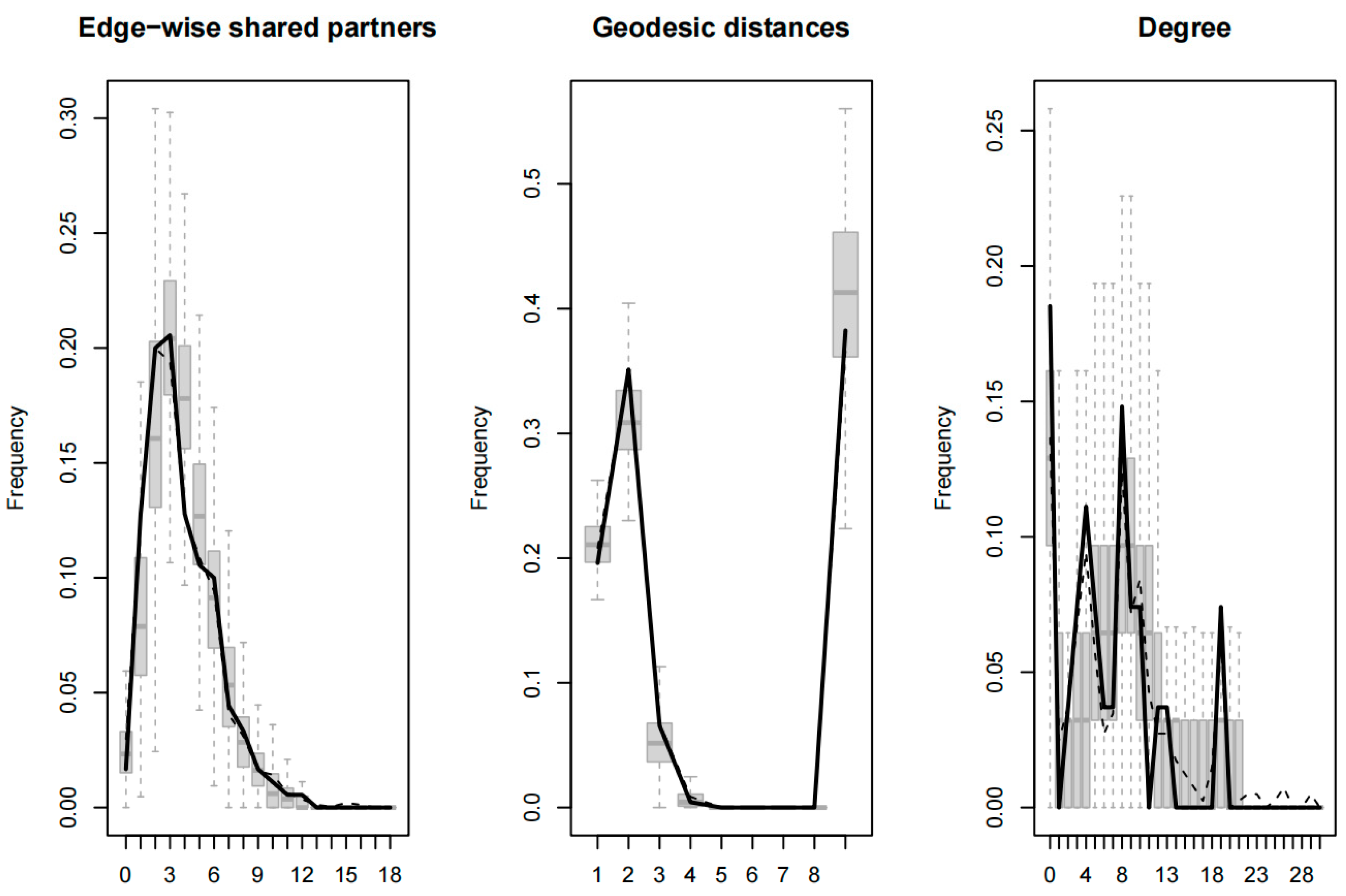
To check the accuracy of Model 4, a simulated network that has the same statistical characteristics as the actual network is commonly used. This process involves creating multiple simulated networks with similar structural characteristics and comparing them to the actual network’s structural characteristics to determine the effectiveness of the method. The characteristic estimates of the simulated network are then used to create a box plot. A good model-fitting effect is indicated when the median value is closer to the characteristic estimates obtained from the actual network.
To evaluate the effectiveness of the fitting of a network, it is important to observe certain statistics. Figure 10 displays the results of observing three crucial statistics. The black line in the diagram represents the actual network, while the box plot depicts a random network. Upon analyzing the fitting graph of edge-wise shared partners, it is evident that the black line is mostly positioned close to the middle of the box diagram, indicating satisfactory fitting results. Similarly, the fitting of geodesic distances and degree also prove to be ideal.
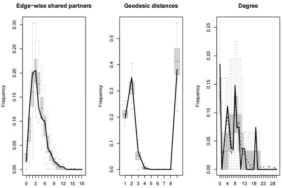
Figure 10.
GOF test results.
4.3.4. Heterogeneity Test
The spatial correlation network of transportation carbon emission intensity is divided into three stages according to time nodes, namely 2008–2012, 2013–2017, and 2018–2021, to explore the network time heterogeneity in three different periods of social development. According to the results, it can be seen that the direction and significance of the estimated coefficients of the endogenous structure and exogenous mechanism driving factors in the three stages are consistent with Model 4. What is slightly different is that the variability coefficient changed from insignificant to significant from 2018 to 2021. This shows that under the impact of external factors such as the deepening of transportation carbon emission reduction policies, the transportation carbon emission intensity preference relationship tends to disappear in the next period, and the network may become sparse.
5. Conclusions and Policy Recommendations
5.1. Conclusions
This study analyzes China’s provincial transportation carbon emission data from 2008 to 2021. It uses a modified gravity model to develop a spatial correlation network of transportation carbon emission intensity. This study then employs the SNA method to conduct a detailed analysis of its structural characteristics. Using the TERGM, this study empirically examines the evolution mechanism of its spatial correlation network. This research shows that:
- (1)
- The carbon emission intensity of transportation in China’s provinces is unbalanced. In terms of time series, except for Northeast China, other regions generally demonstrate a decreasing trend year by year, and there are significant differences between different provinces. The increase in transportation carbon emission intensity in Northeast China after 2017 may be closely related to the adjustment of its economic structure, as the region shifted from heavy industry to high technology and service industries. This change led to a decrease in the gross value of transportation production and an increase in transportation carbon emission intensity. Regarding spatial distribution, emissions tend to be lower in the East and higher in the West. The Gini coefficient, which measures inequality, has generally decreased. The transportation carbon emission intensity in Northeast China is generally higher than that in East and South China. The spatial distribution of transportation carbon emission intensity in Northeast China has obvious stage characteristics in its changes over time.
- (2)
- The intensity of carbon emissions from transportation is becoming increasingly interconnected between provinces, with a complex spatial correlation network. The national average transportation carbon emission intensity correlation strength increased from 35.81 in 2008 to 495.19 in 2021, showing a distribution pattern of “denser in the East and sparser in the West”. There are no isolated provinces in this network structure, and the transportation carbon emission intensity of provincial nodes has broken through the limitations of geographical proximity. Spatial structure characteristics have emerged around the Beijing–Tianjin–Hebei, Yangtze River Delta, and Pearl River Delta areas. At the same time, there is heterogeneity in the spatial correlation network of transportation carbon emission intensity, and there are obvious differences in the centrality of different provinces.
- (3)
- The intensity of carbon emissions from transportation in different Chinese provinces is unevenly distributed. This disparity is mainly due to the influence of central provinces such as Shanghai, Beijing, Tianjin, Guangdong, and Fujian. These provinces play a vital role in collaborating with other regions to develop low-carbon transportation. They strengthen the interconnections between other provinces through the role of “intermediaries” and “bridges” in the network and occupy a key position in the related network.
- (4)
- Due to the gap in resource endowment and economic development among Chinese provinces, the spatial correlation network of transportation carbon emission intensity shows an obvious clustering phenomenon; that is, there are dense connections between some nodes, while the connections between other nodes are sparse. This clustering characteristic leads to the existence of four major plates in the network: “two-way spillover”, “net benefit”, “broker”, and “net spillover”. This network relationship mainly represents the interactive correlation between plates. The “net benefit” plate primarily includes developed regions, whereas the “net spillover” plate mainly includes less developed regions.
- (5)
- According to the results of the TERGM analysis, the mutual and gwesp indicators in the endogenous structural variables significantly positively impact the formation of the spatial correlation network of transportation carbon emission intensity in Chinese provinces. However, population size, GDP, and green technology level also play an essential role in developing this network. The network exhibits a certain degree of stability and displays a significant stability trend over time.
5.2. Policy Recommendations
Based on the conclusions drawn, the following suggestions should be implemented:
- (1)
- Collaborate on cross-regional and cross-departmental transportation carbon emission reduction strategies and gradually reduce the transportation carbon emission intensity of all provinces across the country. The country must rely on multiple provinces to achieve emission reduction targets. It also needs to explore further paths for emission reduction implementation and safeguard measures based on each province’s population exchanges, economic connections, green technology levels, geographical location, etc. Moreover, it is important to establish a mechanism for cross-regional and cross-departmental transportation carbon emission reduction collaboration governance for healthy development.
- (2)
- We need to use the central provinces’ leading role in the network structure to reduce transportation carbon emissions effectively. Therefore, we should prioritize the implementation of transportation energy-saving and carbon emission reduction technologies in provinces such as Shanghai, Beijing, Tianjin, Guangdong, and Fujian, which are at the center of the network. This will help to maximize their radiation-driving effect. Additionally, we must take active measures to strengthen the interconnection of low-carbon transportation exchanges with the Western region. This will help reduce the transportation carbon emission intensity of provinces on the network’s edge, thus breaking the “Matthew Effect” situation of transportation carbon emission intensity. Ultimately, this will enable a balanced and coordinated development of China’s low-carbon transportation.
- (3)
- According to the spatial correlation characteristics of the plate in which the province is located, targeted measures should be further formulated to promote the connections between and within the plates, focusing on the input of low-carbon transportation resource elements in the provinces within the “net spillover” plate, to fully utilize the resource endowments and socio-economic potential of each province while weakening the gradient differentiation of the network and achieving transportation carbon emission reduction goals in different regions.
Author Contributions
Conceptualization, C.Y., J.Z. (Jinrui Zhu) and S.Z. (Shuai Zhang); Data Curation, J.Z. (Jiannan Zhao); Formal Analysis, J.Z. (Jinrui Zhu); Methodology, C.Y.; Resources, C.Y. and S.Z. (Shuai Zhang); Software, S.Z. (Shibo Zhu); Supervision, C.Y.; Writing—Original Draft, J.Z. (Jinrui Zhu); Writing—Review and Editing, S.Z. (Shuai Zhang) and J.Z. (Jiannan Zhao). All authors have read and agreed to the published version of the manuscript.
Funding
This research was funded by the Natural Science Basic Research Plan in Shaanxi Province of China (grant number No. 2021JC-27) and the Shaanxi Provincial Key Science and Technology Innovation Group (grant number No. 2023-CX-TD-11).
Institutional Review Board Statement
Not applicable.
Informed Consent Statement
Not applicable.
Data Availability Statement
The case analysis data used to support the findings of this study are available from the corresponding author upon request.
Acknowledgments
The authors would like to thank the editors and reviewers for their valuable comments and suggestions on this paper.
Conflicts of Interest
Author Shibo Zhu was employed by the company BYD Automobile Co., Ltd. The remaining authors declare that the research was conducted in the absence of any commercial or financial relationships that could be construed as a potential conflict of interest.
References
- Gurney, K.R. China at the carbon crossroads. Nature 2009, 458, 977–979. [Google Scholar] [CrossRef]
- Mi, Z.; Meng, J.; Guan, D.; Shan, Y.; Song, M.; Wei, Y.-M.; Liu, Z.; Hubacek, K. Chinese CO2 emission flows have reversed since the global financial crisis. Nat. Commun. 2017, 8, 1712. [Google Scholar] [CrossRef] [PubMed]
- Liu, Z.; Guan, D.; Wei, W.; Davis, S.J.; Ciais, P.; Bai, J.; Peng, S.; Zhang, Q.; Hubacek, K.; Marland, G.; et al. Reduced carbon emission estimates from fossil fuel combustion and cement production in China. Nature 2015, 524, 335–338. [Google Scholar] [CrossRef] [PubMed]
- Fan, Y.V.; Perry, S.; Klemeš, J.J.; Lee, C.T. A review on air emissions assessment: Transportation. J. Clean. Prod. 2018, 194, 673–684. [Google Scholar] [CrossRef]
- Lim, S.; Lee, K.T. Implementation of biofuels in Malaysian transportation sector towards sustainable development: A case study of international cooperation between Malaysia and Japan. Renew. Sustain. Energy Rev. 2012, 16, 1790–1800. [Google Scholar] [CrossRef]
- Yan, Z. White Paper on Zero Carbon Urban Transportation. Ph.D. Thesis, Tsinghua University Internet Industry Research Institute, Beijing, China, 2022. [Google Scholar]
- Liu, Z.; Li, L.; Zhang, Y.-J. Investigating the CO2 emission differences among China’s transport sectors and their influencing factors. Nat. Hazards 2015, 77, 1323–1343. [Google Scholar] [CrossRef]
- Gasparatos, A.; El-Haram, M.; Horner, M. A longitudinal analysis of the UK transport sector, 1970–2010. Energy Policy 2009, 37, 623–632. [Google Scholar] [CrossRef]
- State Council of China. The “14th Five-Year Plan” for the Development of Green Transportation. 2021. Available online: https://www.gov.cn/zhengce/zhengceku/2022-01/21/content_5669662.htm (accessed on 15 June 2023). (In Chinese)
- Wang, C.; Wood, J.; Wang, Y.; Geng, X.; Long, X. CO2 emission in transportation sector across 51 countries along the Belt and Road from 2000 to 2014. J. Clean. Prod. 2020, 266, 122000. [Google Scholar] [CrossRef]
- Yu, Y.; Li, S.; Sun, H.; Taghizadeh-Hesary, F. Energy carbon emission reduction of China’s transportation sector: An input–output approach. Econ. Anal. Policy 2021, 69, 378–393. [Google Scholar] [CrossRef]
- Zhou, D.; Huang, F.; Wang, Q.; Liu, X. The role of structure change in driving CO2 emissions from China’s waterway transport sector. Resour. Conserv. Recycl. 2021, 171, 105627. [Google Scholar] [CrossRef]
- Wang, L.; Zhang, M.; Song, Y. Research on the spatiotemporal evolution characteristics and driving factors of the spatial connection network of carbon emissions in China: New evidence from 260 cities. Energy 2024, 291, 130448. [Google Scholar] [CrossRef]
- Zhang, N.; Zhang, Y.; Chen, H. Spatial Correlation Network Structure of Carbon Emission Efficiency of Railway Transportation in China and Its Influencing Factors. Sustainability 2023, 15, 9393. [Google Scholar] [CrossRef]
- He, Y.-Y.; Wei, Z.-X.; Liu, G.-Q.; Zhou, P. Spatial network analysis of carbon emissions from the electricity sector in China. J. Clean. Prod. 2020, 262, 121193. [Google Scholar] [CrossRef]
- Pan, A.; Xiao, T.; Dai, L. The structural change and influencing factors of carbon transfer network in global value chains. J. Environ. Manag. 2022, 318, 115558. [Google Scholar] [CrossRef] [PubMed]
- Li, X.; Lv, T.; Zhan, J.; Wang, S.; Pan, F. Carbon Emission Measurement of Urban Green Passenger Transport: A Case Study of Qingdao. Sustainability 2022, 14, 9588. [Google Scholar] [CrossRef]
- Ji, Y.; Dong, J.; Jiang, H.; Wang, G.; Fei, X. Research on carbon emission measurement of Shanghai expressway under the vision of peaking carbon emissions. Transp. Lett. 2023, 15, 765–779. [Google Scholar] [CrossRef]
- Yuan, R.-Q.; Tao, X.; Yang, X.-L. CO2 emission of urban passenger transportation in China from 2000 to 2014. Adv. Clim. Change Res. 2019, 10, 59–67. [Google Scholar] [CrossRef]
- Li, X.; Yu, B. Peaking CO2 emissions for China’s urban passenger transport sector. Energy Policy 2019, 133, 110913. [Google Scholar] [CrossRef]
- Lu, Q.; Chai, J.; Wang, S.; Zhang, Z.G.; Sun, X.C. Potential energy conservation and CO2 emissions reduction related to China’s road transportation. J. Clean. Prod. 2020, 245, 118892. [Google Scholar] [CrossRef]
- Hai-xia, F.; Xing-yu, W.; Hua-cai, X.; Xin-hua, L.; Jian, L.; Er-wei, N. Impact of Urban Traffic Operations on Vehicle Carbon Dioxide Emission. J. Transp. Syst. Eng. Inf. Technol. 2022, 22, 167–175. [Google Scholar] [CrossRef]
- He, D.; Liu, H.; He, K.; Meng, F.; Jiang, Y.; Wang, M.; Zhou, J.; Calthorpe, P.; Guo, J.; Yao, Z.; et al. Energy use of, and CO2 emissions from China’s urban passenger transportation sector—Carbon mitigation scenarios upon the transportation mode choices. Transp. Res. Part A Policy Pract. 2013, 53, 53–67. [Google Scholar] [CrossRef]
- Réquia, W.J.; Koutrakis, P.; Roig, H.L. Spatial distribution of vehicle emission inventories in the Federal District, Brazil. Atmos. Environ. 2015, 112, 32–39. [Google Scholar] [CrossRef]
- Shu, Y.; Lam, N.S.N. Spatial disaggregation of carbon dioxide emissions from road traffic based on multiple linear regression model. Atmos. Environ. 2011, 45, 634–640. [Google Scholar] [CrossRef]
- Huang, Z.; Cao, F.; Jin, C.; Yu, Z.; Huang, R. Carbon emission flow from self-driving tours and its spatial relationship with scenic spots—A traffic-related big data method. J. Clean. Prod. 2017, 142, 946–955. [Google Scholar] [CrossRef]
- Li, F.; Cai, B.; Ye, Z.; Wang, Z.; Zhang, W.; Zhou, P.; Chen, J. Changing patterns and determinants of transportation carbon emissions in Chinese cities. Energy 2019, 174, 562–575. [Google Scholar] [CrossRef]
- Yuan, C.-W.; Qiao, D.; Yang, Y.-F.; Rui, X.-L. Spatial differentiation and clustering analysis of transportation carbon emission intensity in Chinese provinces. Environ. Eng. 2018, 36, 185–190. [Google Scholar] [CrossRef]
- Fu, X. Carbon emission efficiency measurement and spatial characteristics analysis of transportation industry in Yangtze River Economic Zone. Logist. Eng. Manag. 2023, 45, 95–98+119. [Google Scholar]
- Hu, Y.; Yu, Y.; Mardani, A. Selection of carbon emissions control industries in China: An approach based on complex networks control perspective. Technol. Forecast. Soc. Chang. 2021, 172, 121030. [Google Scholar] [CrossRef]
- Bai, C.; Zhou, L.; Xia, M.; Feng, C. Analysis of the spatial association network structure of China’s transportation carbon emissions and its driving factors. J. Environ. Manag. 2020, 253, 109765. [Google Scholar] [CrossRef]
- Zhang, S.; Yuan, C.; Zhao, X. Spatial clustering and correlation network structure analysis of transportation carbon emissions in China. Econ. Geogr. 2019, 39, 122–129. [Google Scholar] [CrossRef]
- Jiang, M.; An, H.; Gao, X.; Liu, S.; Xi, X. Factors driving global carbon emissions: A complex network perspective. Resour. Conserv. Recycl. 2019, 146, 431–440. [Google Scholar] [CrossRef]
- Dong, J.; Li, C. Structure characteristics and influencing factors of China’s carbon emission spatial correlation network: A study based on the dimension of urban agglomerations. Sci. Total Environ. 2022, 853, 158613. [Google Scholar] [CrossRef] [PubMed]
- Ma, F.; Wang, Y.; Yuen, K.F.; Wang, W.; Li, X.; Liang, Y. The Evolution of the Spatial Association Effect of Carbon Emissions in Transportation: A Social Network Perspective. Int. J. Environ. Res. Public Health 2019, 16, 2154. [Google Scholar] [CrossRef] [PubMed]
- Broekel, T.; Balland, P.-A.; Burger, M.; van Oort, F. Modeling knowledge networks in economic geography: A discussion of four methods. Ann. Reg. Sci. 2014, 53, 423–452. [Google Scholar] [CrossRef]
- Contractor, N.S.; Wasserman, S.; Faust, K. Testing multi-theoretical multilevel hypotheses about organizational networks: An analytic framework and empirical example. Acad. Manag. Rev. 2006, 31, 681–703. [Google Scholar] [CrossRef]
- Hunter, D.R.; Handcock, M.S.; Butts, C.T.; Goodreau, S.M.; Morris, M. ergm: A Package to Fit, Simulate and Diagnose Exponential-Family Models for Networks. J. Stat. Softw. 2008, 24, nihpa54860. [Google Scholar] [CrossRef] [PubMed]
- Xiong, J.; Feng, X.; Tang, Z. Understanding user-to-User interaction on government microblogs: An exponential random graph model with the homophily and emotional effect. Inf. Process. Manag. 2020, 57, 102229. [Google Scholar] [CrossRef]
- Holland, P.W.; Leinhardt, S. An Exponential Family of Probability Distributions for Directed Graphs. J. Am. Stat. Assoc. 1981, 76, 33–50. [Google Scholar] [CrossRef]
- Frank, O.; Strauss, D. Markov Graphs. J. Am. Stat. Assoc. 1986, 81, 832–842. [Google Scholar] [CrossRef]
- Golding, P.; Murdock, G. Theories of Communication and Theories of Society. Commun. Res. 1978, 5, 339–356. [Google Scholar] [CrossRef]
- Hanneke, S.; Fu, W.; Xing, E.P. Discrete temporal models of social networks. Electron. J. Stat. 2010, 4, 585–605, 521. [Google Scholar] [CrossRef]
- Yan, R.; Chen, M.; Xiang, X.; Feng, W.; Ma, M. Heterogeneity or illusion? Track the carbon Kuznets curve of global residential building operations. Appl. Energy 2023, 347, 121441. [Google Scholar] [CrossRef]
- Yan, R.; Ma, M.; Zhou, N.; Feng, W.; Xiang, X.; Mao, C. Towards COP27: Decarbonization patterns of residential building in China and India. Appl. Energy 2023, 352, 122003. [Google Scholar] [CrossRef]
- Shao, H.; Wang, Z. Spatial correlation network structure of transportation carbon emission efficiency in China and its influencing factors. China Popul. Resour. Environ. 2021, 31, 32–41. [Google Scholar]
- Xu, H.; Li, Y.; Zheng, Y.; Xu, X. Analysis of spatial associations in the energy–carbon emission efficiency of the transportation industry and its influencing factors: Evidence from China. Environ. Impact Assess. Rev. 2022, 97, 106905. [Google Scholar] [CrossRef]
- Dong, S.; Ren, G.; Xue, Y.; Liu, K. Urban green innovation’s spatial association networks in China and their mechanisms. Sustain. Cities Soc. 2023, 93, 104536. [Google Scholar] [CrossRef]
- Chen, Q. Study on Urban economic region of Huaihai Economic Region Based on Economic Contacts. Urban Stud. 2009, 5, 18–23. [Google Scholar]
- Wang, Q.Q.; Huang, X.J.; Chen, Z.G.; Tan, D.; Chuai, X.W. Movement of the Gravity of Carbon Emissions Per Capita and Analysis of Causes. J. Nat. Resour. 2009, 24, 833–841. [Google Scholar] [CrossRef]
- Song, J.; Feng, Q.; Wang, X.; Fu, H.; Jiang, W.; Chen, B. Spatial Association and Effect Evaluation of CO2 Emission in the Chengdu–Chongqing Urban Agglomeration: Quantitative Evidence from Social Network Analysis. Sustainability 2019, 11, 1. [Google Scholar] [CrossRef]
- Setiawan, A.; Jufri, F.H.; Dzulfiqar, F.; Samual, M.G.; Arifin, Z.; Angkasa, F.F.; Aryani, D.R.; Garniwa, I.; Sudiarto, B. Opportunity Assessment of Virtual Power Plant Implementation for Sustainable Renewable Energy Development in Indonesia Power System Network. Sustainability 2024, 16, 1721. [Google Scholar] [CrossRef]
- Gan, J.; Zhang, D.; Guo, F.; Dong, E. Intensity of Tourism Economic Linkages in Chinese Land Border Cities and Network Characterization. Sustainability 2024, 16, 1843. [Google Scholar] [CrossRef]
- Hu, S.; Wu, X.; Cang, Y. Exploring Business Environment Policy Changes in China Using Quantitative Text Analysis. Sustainability 2024, 16, 2159. [Google Scholar] [CrossRef]
- Li, Z.; Sun, L.; Geng, Y.; Dong, H.; Ren, J.; Liu, Z.; Tian, X.; Yabar, H.; Higano, Y. Examining industrial structure changes and corresponding carbon emission reduction effect by combining input-output analysis and social network analysis: A comparison study of China and Japan. J. Clean. Prod. 2017, 162, 61–70. [Google Scholar] [CrossRef]
- Wang, F.; Gao, M.; Liu, J.; Fan, W. The Spatial Network Structure of China’s Regional Carbon Emissions and Its Network Effect. Energies 2018, 11, 2706. [Google Scholar] [CrossRef]
- White, H.C.; Boorman, S.A.; Breiger, R.L. Social Structure from Multiple Networks. I. Blockmodels of Roles and Positions. Am. J. Sociol. 1976, 81, 730–780. [Google Scholar] [CrossRef]
- Cai, H.; Wang, Z.; Zhu, Y. Understanding the structure and determinants of intercity carbon emissions association network in China. J. Clean. Prod. 2022, 352, 131535. [Google Scholar] [CrossRef]
- Dey, C.J.; Quinn, J.S. Individual attributes and self-organizational processes affect dominance network structure in pukeko. Behav. Ecol. 2014, 25, 1402–1408. [Google Scholar] [CrossRef]
- Brashears, M.E. Exponential Random Graph Models for Social Networks: Theory, Methods, and Applications. Contemp. Sociol. 2014, 43, 552–553. [Google Scholar] [CrossRef]


Disclaimer/Publisher’s Note: The statements, opinions and data contained in all publications are solely those of the individual author(s) and contributor(s) and not of MDPI and/or the editor(s). MDPI and/or the editor(s) disclaim responsibility for any injury to people or property resulting from any ideas, methods, instructions or products referred to in the content. |
© 2024 by the authors. Licensee MDPI, Basel, Switzerland. This article is an open access article distributed under the terms and conditions of the Creative Commons Attribution (CC BY) license (https://creativecommons.org/licenses/by/4.0/).