Abstract
Precooling agricultural produce is an intensive, energy-consuming process. To improve the efficiency of forced-air precooling and ultimately contribute to energy sustainability for postharvest storage of fresh produce, we designed three alternative air supply systems, simulated their cooling performances over a 96 h precooling process in a cold storage facility storing Chinese cabbages, and then compared their performances with a conventional design. All models were developed on a large scale on the basis of validated computational fluid dynamics models. The horizontal air supply scheme shortened the seven-eighths cooling time by 18.8%, and its maximum cooling rate increased by 19.7% compared to the conventional air supply scheme. The seven-eighths cooling time under another alternative design, the vertical air supply scheme, was 9.4% lower than the conventional, with the maximum cooling rate increasing by 10.5%. However, the maximum cooling rate of the last alternative design, the perforated ceiling air supply system, was 6.6% less than the conventional scheme, resulting in a 6.3% longer seven-eighths cooling time. The heterogeneity index of temperature implied that the horizontal air supply offered better overall cooling uniformity than the other designs, which can be attributed to its evenly distributed airflows and well-organized air movement paths, based on the combined analysis of temperature contours and air velocity contours at selected planes. Our findings are expected to provide practical guidelines for the refinement of the air supply system to improve its energy sustainability in forced-air precooling.
1. Introduction
Sustainability is one of the biggest challenges facing the agriculture and food sectors [1]. Energy is required at every stage of the food value chain, from production in the field to marketing and consumption. One of the most energy-intensive processes is precooling, which removes field heat from agricultural products immediately after harvest [2,3]. Rapidly cooling fresh produce to an optimal temperature is crucial for long-term storage and cold chain transportation, even though it costs considerable energy to accomplish. Low temperatures can effectively prevent the deterioration of produce by slowing down physiological and metabolic activities, such as respiration rate, which has a significant impact on maintaining product quality, extending shelf life, and reducing weight loss [3,4].
Although various techniques are available for precooling, forced-air cooling is more widely used than any other precooling technique since it is more versatile and efficient to cool palletized produce on a large scale [5,6,7]. Forced-air cooling is facilitated by evaporators and fans to remove heat through convective heat transfer between ambient air and produce. A driving force is generated by the pressure difference across packaging so that cooling air can be drawn, forming internal air circulations. The packaging of produce plays an impactful role in precooling performance. Therefore, many studies have focused on optimizing vented packaging for specific agricultural products [5,6,8,9]. However, the efficiency of forced-air precooling is determined by not only the design of packages but also how the cooling air is supplied and distributed.
The air supply system lacks recognition, even though it is an indispensable component for the forced-air precooling process. In fact, indoor airflow patterns have a huge impact on cooling performance, which determines the efficiency of cooling and energy use. An optimal air supply scheme maximizes the field heat removal rate and plays a pivotal role in creating efficient cooling airflows [10]. Furthermore, cooling uniformity is always highly required as a critical parameter to assess pre-cooling performance [2,6]. In addition, cooling air speeds should fall within a desired range to avoid unnecessary weight loss of products during precooling [11,12]. Hence, optimizing air supplies to provide accurate and sufficient airflows for forced-air precooling is of great significance to improving cooling performance. This optimization also benefits the saving of capital costs, such as possible equipment downsizing, as well as reducing total energy consumption to enhance sustainability during the post-harvest processing of agricultural produce.
Common air supply designs used in cold storage are simple ventilation features that are inexpensive and easy to install [13,14,15]. For example, separate diffusers (inlets and outlets) or inlets of evaporator units can almost meet the regular demand for precooling. However, one of the biggest drawbacks of conventional air supply systems is a severe lack of airflow accuracy. As a result, unevenly distributed temperatures, air stratification, and excessive air movements in partial areas may occur and cause unsustainable energy consumption [14,16,17,18].
Precise and efficient air supply designs are necessary to improve the performance of the forced-air precooling process and eventually improve sustainable energy use [4,7]. Recently, air ducting has been widely used as air supplies in HVAC applications, particularly in controlled environment agriculture, livestock farming, and food processing [17,19,20,21,22]. Compared to conventional air supplies, air ducts are more manageable in precisely distributing airflows [23]. Because air ducts are very versatile in terms of materials and types and have relatively low costs, they can be manufactured according to specific applications and are handy for installation, replacement, and maintenance [24]. For precooling, a duct-based air supply system does not need extra space to install and can be directly connected to existing inlets. Paths of air ducting can be planned based on the layout of cargo, and vice versa. Note that air ducts made of fabric and polyvinyl chloride are usually prevalent in environments with low temperatures and high humidity.
In addition to air ducts, Guo et al. compared the precooling performance of three air supply schemes: single inlets, double inlets, and a perforated ceiling [25]. The embedded attic space above the ceiling contains incoming cooling air and creates a pressure difference that drives the cold air to enter the space underneath, where fresh produce is placed through small holes in the ceiling. Their results suggested that the perforated ceiling air supply had the most uniform temperature distribution compared to the other two designs due to finely directed top-to-bottom cooling airflows, while the comparisons of precooling rates were not disclosed.
To assess indoor environmental conditions and ventilation system performance, investigators usually combine computer modeling with field tests [2,4]. Computational fluid dynamics (CFD) is a sophisticated modeling method that is widely used in many fields [26,27]. The number of CFD studies addressing agricultural issues has grown vastly during the past three decades [26]. Using CFD simulations to study postharvest storage problems of horticultural produce has been demonstrated as an efficient and accurate approach [4]. Hoang et al. employed CFD modeling to simulate airflows in a cold storage room to investigate indoor climate and its relationship with evaporator positioning [28]. Later, they used transient simulations to characterize temperature and airflow distributions with and without produce [29]. A similar study was conducted to compare airflow patterns and temperature distribution uniformity in cold storage with a slot-ventilated ceiling both before and after loading produce [30,31].
Several previous studies have adopted CFD simulations to investigate air supply designs for precooling. Shen et al. simulated the indoor environment of an empty cold storage with a perforated ceiling [32]. Their findings revealed the uniformity of internal airflows was significantly improved compared to the conventional air supply, while changing the inlet velocity did not show much impact on indoor airflows. Moureh and the group simulated airflow patterns and temperature distributions in a loaded refrigeration truck [33,34]. Their later results implied that using air ducts could increase the efficiency of cooling and reduce stagnant zones by improving airflow uniformity, which is beneficial for maintaining produce quality during transportation [34]. Another CFD study conducted by Liu and Nan investigated air ducting in a commercial cold storage facility loaded with apples [10]. In their study, a 16.1 m air duct with 50 round symmetrical perforations on both sides was designed. To ensure uniform air speed at each individual perforation, the duct size decreased gradually from the evaporator-proximal end to the far end. Based on their conclusions, the non-uniformity coefficient of temperature and relative humidity were both decreased by about 20%, while the air diffusion performance index (ADPI) was increased by 11.1% using air ducts compared to the control. There are some other studies using CFD modeling to evaluate and compare the performance of air ducting systems with specific applications [17,24,35], although scarce investigations were performed to systematically compare the precooling performance between multiple air supply schemes.
This study aims to investigate air supply options for a typical precooling facility to optimize its cooling performance via CFD simulations. Based on a validated CFD model, the control-type and three alternative air supply systems were modeled accordingly. We compared the simulation results of three alternative air supply systems to the control model by analyzing key parameters, including cooling time, cooling rate, and cooling uniformity within the same storage room. Our goal is to explain the different performances of air supply options based on their indoor airflow patterns and provide recommendations for the refinement of precooling air supply designs. Therefore, an optimized air supply system should work concurrently with other factors, like packaging designs, to achieve an improved energy-sustainable solution for postharvest produce precooling.
2. Materials and Methods
One typical forced-air precooling cold storage system with a conventional air supply scheme and three alternative air supply systems were investigated, with corresponding CFD models developed. The CFD model representing conventional air supply was appointed as the control type and validated with experimental measurements, which were subsequently adopted for the development of the three alternative models to compare precooling performance. Two of the three alternatives are air duct-based, while the third one has air supplies facilitated by a perforated ceiling.
2.1. The Study of Cold Storage Facilities
This study was conducted at a cold storage facility located at the National Engineering Research Center for Preservation of Agricultural Products in Tianjin, China. The cold storage room had an asymmetric layout and a concrete floor and was 696 cm long, 446 cm wide, and 268 cm high, with a total volume of 66 m3 and a total floor area of approximately 28.8 m2 (Figure 1A). Fresh produce was stocked on shelves that had wire-mesh surfaces that allowed airflow to go through vertically. All the walls and the flat ceiling were all made of aluminum.
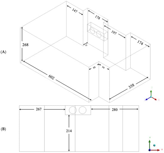
Figure 1.
Dimensions of the study cold storage room with the control-type air supply system (unit: cm). (A) Isometric view. (B) Front view.
The study cold storage room was equipped with an evaporator mounted 214 cm above the floor and 50 cm away from the back wall, which is commonly used in cold storage facilities, namely, the control type (Figure 1B). The dimension of the evaporator unit was 150 × 50 × 30 cm, with its top surface attached to the ceiling. The distance between the evaporator and two sidewalls was 267 cm to the left and 280 cm to the right, respectively. Two identical fans, each with a diameter of 40 cm, were responsible for introducing cooling air at the front, while the entire back of the evaporator unit was used as return vents connected to exhaust ducts. The operation of the evaporator was automatically regulated by a control panel based on settings and instantaneous readings of the indoor temperature.
2.2. Alternative Air Supply Systems
Two air ducting systems were designed to refine the conventional air supply system, namely, the horizontal air supply (HAS) and vertical air supply (VAS) systems. Both designs had two 260 cm long air ducts that were directly connected to the fans at one end and fully sealed at the other end. The diameters of the air ducts were the same as those of the connected fans, and the distance between the two ducts was 15 cm. In addition, four identical holes with 10 cm diameters were created at each duct every 50 cm to introduce cooling air, and each hole had the same opening size of 78.50 cm2. The only difference between HAS and VAS was the location of air holes, which led to horizontal and vertical incoming airflows.
The third alternative was designed to represent a perforated ceiling air supply (PCAS) system. Inspired by previous investigations, we added an extra ceiling to the study cold storage, which also had a vertical board connected to the front surface, and its bottom was aligned with the bottom of the evaporator unit. Thus, an enclosed attic area was formed, which allowed the incoming cooling air to be mixed prior to entering the underneath space. In total, 30 perforations with 10 cm diameters were created as air supply holes on the additive ceiling that were evenly distributed. The distance between those holes in the same row was 50 cm, while two adjacent rows of holes had a gap of 120 cm.
2.3. Development of the CFD Model
Indoor environmental conditions were simulated using the commercial software package FLUENT [36] by developing four three-dimensional models that were correlated to the four air supply schemes (control, HAS, VAS, and PCAS). With the simulation outputs, precooling performances were evaluated using criteria accordingly.
2.3.1. Computational Domains
All CFD models have similar computational domains that were developed based on the actual geometry of the study cold storage room. All four models were constructed on a large-scale to represent the same facility with different air supply systems (Figure 2). To assess their precooling performances, 60 corrugated fiberboard boxes full of Chinese cabbage were modeled, each with dimensions of 60 × 60 × 50 cm. In addition, two hand holes were created for each box on two sides, with an opening size of 44.5 cm2 each.
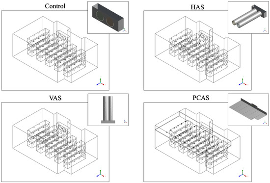
Figure 2.
Illustrations of the computational domain of four models: Control, HAS, VAS, and PCAS, respectively, with specific air supply systems annotated at the upper right.
2.3.2. Preconditions and Assumptions
The cold storage was considered ideally insulated, assuming no infiltration. Indoor gases were modeled as a mixture of air and water vapor, which were presumed to be incompressible ideal gases. The temperature and humidity of the initial cooling air were assumed to be constant. In addition, no chemical reaction or phase change was included in the simulations, as the cooling process was mainly dependent on convective heat transfer. Due to negligible effects on airflows, the body of shelves was not modeled as another simplification. Four boxes at the same level of one shelf were assumed to be tightly placed with no space between them. All boxes were modeled as solids, assuming they were full of Chinese cabbages with zero spare space. Note that sensible or latent heat generated by Chinese cabbage was not modeled in this study, while its thermal conductivity was assumed to be constant.
2.3.3. Model Configurations
The geometry drawing and three-dimensional domain construction were performed using commercial codes embedded in ANSYS packages. Unstructured mesh was generated for all four models using ANSYS-Meshing. Grid skewness was chosen as a critical index to assess the meshing quality prior to simulations. Additionally, a standard mesh convergence study was performed to verify meshing integrity and sufficiency of mesh refinement using the Grid Convergence Index (GCI) [37]. Three mesh scales of the control model were created, including 830,150, 1,469,272, and 4,005,975 cells. The GCI value was analyzed and compared at three selected points, which turned out to be declining when the meshing scale increased, indicating the grid was successfully refined (Supplementary Materials). However, the largest size of meshing was not computationally efficient considering the refinement it provided versus the more computing time it demanded. Therefore, the median meshing scale was adopted to continue subsequent model development. The final mesh sizes of control, HAS, VAS, and PCAS were 1,469,272, 1,583,385, 1,582,310, and 1,568,130, respectively. For all four models, the minimum cell generated in mesh varied between 7.2 × 10⁻⁷ and 1.8 × 10⁻⁶ m3, while the maximum cell size was around 0.02 m3.
The Reynolds-averaged Navier-Stokers (RANS) equations were solved in each cell using FLUENT solver, incorporating the enhanced wall functions. The standard k-e turbulence model was adopted to scrutinize turbulence-induced instability [38]. A transient mode calculation was performed using a time step of 7200 s to simulate indoor environmental conditions during the precooling process. The convergence criteria were set as 1 × 10⁻⁶ for energy and 1 × 10⁻⁴ for other variables. The indoor airflows were considered stable when air speeds at selected points fluctuated within 1% between time steps. A total of 48 time steps were computed in 2400 iterations. Note that the initial temperature of all cell zones, including the Chinese cabbages, was set at 25 °C prior to the commencement of the precooling process.
2.3.4. Boundary Conditions
The same boundary conditions were applied in four CFD models. The faces of dual evaporator fans were modeled as inlets with a constant mass flow rate of 2.4 kg/s each, serving incoming air at 0.5 °C with a constant mass fraction of 0.006. The entire back of the evaporator unit was defined as a pressure outlet through which indoor air exits into the atmosphere. All boxes of produce were modeled as solid blocks, whereas the interior of each box was defined as solid cell zones to represent Chinese cabbages. The density, specific heat, and thermal conductivity of Chinese cabbage used in modeling were referenced and estimated, as shown in Table 1 [39,40,41]. The surface of each box was assigned the thermal parameters of corrugated fiberboard and was modeled as non-slip walls. In addition, the surrounding walls, floor, ceiling of the storage room, air ducts, and perforated ceiling were all modeled as no-slip aluminum walls without roughness (Table 1).

Table 1.
Geometric features and materials with corresponding thermal properties.
2.3.5. Simulation Data Post-Processing and Evaluation
Three two-dimensional planes, namely Plane-F, Plane-M, and Plane-B, were created to represent the produce locations at the front, middle, and back, respectively. These selected planes were lined up parallelly with 1 m between each other along the z-axis (Figure 3A). Note that Plan-F and Plane-M do not cross any air holes in alternative models, but Plane-B crosses the evaporator unit in all four models due to its designate position. Contours of temperature and air velocity vectors were created using these planes to illustrate indoor environmental conditions and evaluate cooling performances. On each plane, a cross-section of all 15 rows of produce was examined to monitor the temperature variations of the internal Chinese cabbages at different timestamps. The produce was labeled alphabetically from left to right across five stacks (Figure 3B). Within each stack of boxes, the produce was further annotated with numbers 1 to 3 to indicate increasing heights (Figure 3B).
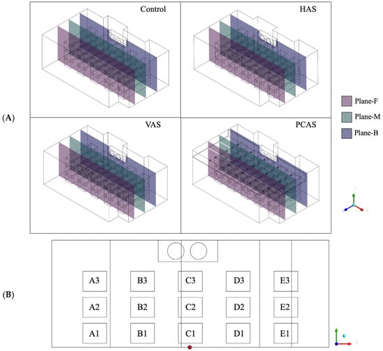
Figure 3.
(A) Three cross-sectional planes highlighted in each model: Plane-F (z = −1.4), Plane-M (z = −2.4), and Plane-B (z = −3.4); (B) A front view of 15 rows of produce with annotations. The origin was marked by the red dot.
The precooling performances of four air supply systems were evaluated using three criteria: cooling time, cooling rate, and cooling uniformity. The half cooling time (HCT) and seven-eighths cooling time (SECT) serve as two critical indices for assessing the cooling time in commercial forced-air facilities. Both values are derived from the temperature profiles, as explained by the following equation:
where the dimensionless temperature change fraction () represents the ratio of unaccomplished temperature change to the anticipated total temperature change at a given time, which is calculated using (K) the cooling air temperature, (K) is the temperature of the initial produce temperature, and is the produce temperature [3]. In this study, was calculated as the volume-weighted average temperature of the Chinese cabbage (Equation (2)).
Thereby, HCT and SECT stood for the time needed to complete a temperature change by half () and seven-eighths () of the anticipated total temperature change, respectively.
During the precooling process, the rate of cooling decreases as the temperature of the produce approaches the cooling air temperature (). To quantify the cooling rate at time , an instantaneous cooling rate was adopted, which is defined as follows [3,4,42]:
where is the cooling coefficient (h−1) that equals the magnitude of the slope of versus , and indicates the instantaneous produce temperature at that is also calculated using Equation (2).
To quantitatively evaluate the cooling uniformity, the heterogeneity index (HI) of temperature was adopted as an indicator of the instantaneous cooling disparities among the produce at various locations [43]. The HI of temperature is defined as follows:
where is the average temperature of all produce at a specific timestamp, and represents the instantaneous temperature of a specific row calculated by the volume-weighted average temperature.
2.3.6. Field Measurement
Measurements of air temperature, relative humidity, and air velocity were taken at 16 sampling locations within the study cold storage without loading produce for two days (24 June 2023 and 27 June 2023). The evaporator was turned on in the early morning while the measurements were conducted in the afternoon to make sure the indoor environment had reached a steady state prior to data recording. Air temperature and relative humidity were measured and recorded using a Testo 480 digital meter with an IAQ probe (Testo, Lenzkirch, Germany) with a sampling rate of one reading per second. The accuracy of the IAQ probe is ±0.3 °C for temperature and ±2% for relative humidity. When the readings of temperature and relative humidity reached a plateau, the indoor climate was considered stable. The indoor air velocity was measured at each sampling location using a Testo 0635-1543 hot wire anemometer (Testo, Lenzkirch, Germany) that has an accuracy of ±4% of reading and ±0.03 m/s. The anemometer was placed vertically to capture the predominant horizontal air movement. When the evaporator is operating, the reading of air velocity at a location usually fluctuates more or less. Therefore, an average of 30 consecutive readings was calculated at a certain sampling location with three repeated measurements for the same spot.
2.3.7. Model Validation
To validate model accuracy, an electric heater (SINFUN, Ningbo, China) was deployed and modeled as the sole heating source in the cold storage, which allowed us to compare prediction results with field measurements using corresponding simulation data in terms of temperature, relative humidity, and air velocity. Note that the measured air velocity was compared with simulated air velocity along the z-axis since the anemometer only captured the horizontal air velocities. Details of field measurement and validation data analysis can be found in the Supplementary Materials.
Several statistical parameters were used as indicators to assess the CFD model performance, including fractional bias (FB), geometric mean bias (MG), geometric mean-variance (), fraction within a factor of two (), and normalized mean square error () [44,45,46]. All equations used to calculate those parameters were listed and described in the Supplementary Materials. Each parameter must fall within a specific range to be deemed acceptable: < 0.3, 0.7 < < 1.3, < 4.0, 0.5 < < 2.0, and < 0.25. A model has to meet more than half of the criteria for those parameters to be considered sufficiently accurate.
3. Results
3.1. Model Validation
In general, the CFD model can provide accurate predictions, as evidenced by adequate agreements between field measurements and simulation results in terms of temperature, air velocity, and relative humidity data (Figure 4). At 16 locations, the simulated results for temperature and relative humidity demonstrated superior alignment with field measurements compared to the air velocity data, with relative errors of 8% and 5% on average, respectively. However, the predicted air velocity had an average relative error of 20%, with the highest value around 58%. The discrepancy in air velocity data could be attributed to the fact that only horizontal air velocity was measured and had a relatively small magnitude.
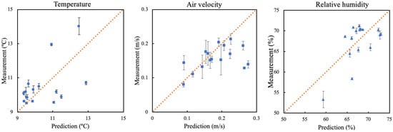
Figure 4.
Comparisons between field measurements and predicted results of temperature, air velocity, and relative humidity represented by circles, squares and triangles, respectively. The dashed lines represent the ideal scenario when predictions made by simulations are exactly the same as field measurements. The vertical error bars stand for the standard deviation of replicates of corresponding field measurements at each location.
In addition, the developed CFD model has been proven to meet the evaluation criteria using the five statistical parameters mentioned earlier (Table 2). All the statistical indices fell within the desired range, indicating that the model could accurately predict key indoor environmental parameters. Therefore, the validated model is suitable for modification to investigate multiple air supply systems and their corresponding indoor environmental parameters.
Table 2.
Summary of statistical parameters for model validation performance assessment.
3.2. Precooling Performance Comparison
To thoroughly compare the precooling performance between the four air supply schemes, we evaluated the cooling time for each model to figure out the potential refinement of air supply systems to fulfill the goal of sustainable precooling methods. According to the simulation results of the volume-weighted average temperature of all produce over time, the HAS model showed superior cooling performance, with the temperature dropping much quicker than the others (Figure 5). After 14 h of precooling with HAS, the average temperature of the Chinese cabbages was reduced to 13 °C, nearly achieving half of the anticipated total temperature drop. Furthermore, the mean temperature of all produce reached 3.5 °C after 52 h, according to the prediction of the HAS model, while the control, VAS, and PCAS models had average temperatures of 4.9, 4.0, and 5.3 °C, respectively.
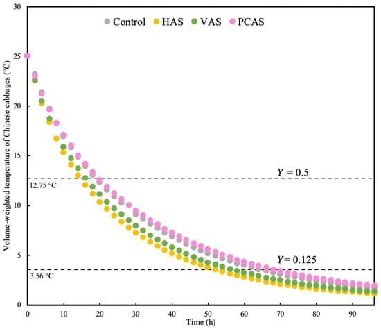
Figure 5.
Cooling time comparison between four models. Plots showing the change in volume-weighted average temperature of Chinese cabbages under each air supply scheme for 96 h based on simulation results. The dash lines indicate anticipated temperatures at HCT and SECT, respectively. Note that the time interval for each data point was 2 h.
The VAS model exhibited the second-best performance with respect to cooling time, as it took slightly more time for all produce to cool down to an average temperature of 12.8 °C. The VAS model needed an additional 6 h to reach 3.6 °C compared to HAS. The control model had a slightly shorter HCT than that of the PCAS model, which reduced the average temperature of all produce below 3.6 °C after 64 h of cooling, and was about 4 h ahead of the PCAS model.
The cooling rate for each design was calculated using Equation (3) and compared to the instantaneous cooling rates at every timestamp (Figure 6). Note that the cooling coefficient for each air supply system was derived from the corresponding simulation data, resulting in a series of constant values of 0.03, 0.04, 0.03, and 0.03 h−1 for the control, HAS, VAS, and PCAS models, respectively. The HAS model possessed the maximum initial cooling rate of 0.9 K/h, followed by the VAS model with an initial cooling rate of 0.8 K/h. The control-type air supply system had an initial cooling rate of 0.8 K/h, which was 7% slightly higher than that of the PCAS model. It is worth noting that the initial cooling rate is directly related to the cooling coefficient.
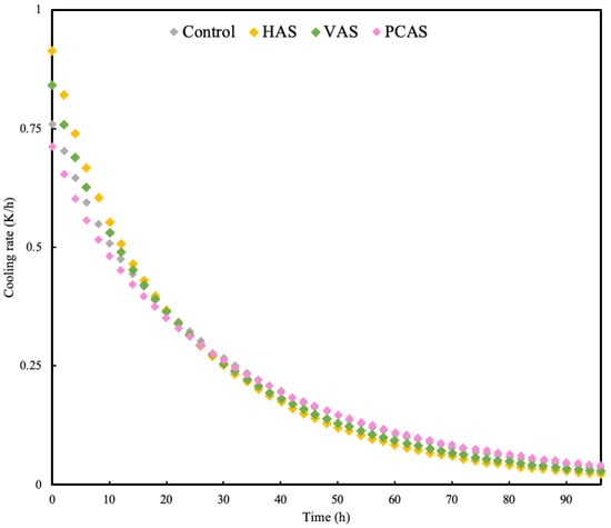
Figure 6.
Comparison of cooling rate changes between four air supply systems for 96 h based on corresponding simulation outputs. Diamonds with different colors represent the instantaneous cooling rate values of each model that were calculated every 2 h using spontaneous predictions.
As the cooling process went on, the instantaneous cooling rates of all models gradually declined (Figure 6). The control model exhibited the maximum instantaneous cooling rate after 22 h, while the cooling rate of the HAS model became the minimum from the 26th hour onwards. Interestingly, all four models had similar instantaneous cooling rates of around 0.3 K/h at the 28th hour of cooling. After 42 h, the PCAS model started to lead to instantaneous cooling rates at each timestamp until the end of the cooling process. By the end of 96 h, the cooling rates of four models had diminished to extremely low levels, with values of 0.04, 0.04, 0.03, and 0.02 for the PCAS, control, VAS, and HAS models, respectively.
Cooling uniformity is another crucial parameter to assess the precooling performance of air supply systems. The instantaneous temperature of Chinese cabbages was compared at various locations with the average temperature during the 96 h precooling process, as well as the dynamic of temperature heterogeneity using HI values (Figure 7). In general, the HI value of the produce at each location increased drastically in the initial hours of cooling and then declined moderately after reaching its peak. Only the produce from the PCAS model presented a moderately fluctuating behavior at the A1 location with a relatively small scale of HI. The maximum instantaneous HI (0.7) was observed at C3 from the simulation results of the VAS model at the 10th hour of precooling, with the minimum HI values observed at several locations for multiple models. For instance, the control model had HI values close to zero at C1, C3, and E3 for most of the precooling process. In addition, the HAS model also displayed nearly flat curves in rows D2 and D3.
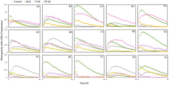
Figure 7.
Plots of heterogeneity index (HI) of average temperature for 15 locations of Chinese cabbages, which were labeled with corresponding row numbers upper right. The x-axis represents cooling time from 0 to 96 h, while the y-axis indicates instantaneous HI values calculated using volume-weighted average temperature at each location. Note that the time interval for each data point was 2 h.
The VAS and PCAS models exhibited extraordinary heterogeneity in terms of instantaneous temperature at multiple locations compared to the control and HAS models. In lower and middle rows like B1, C1, E1, and E2, the VAS model showed higher HI values than any other model from the start of cooling (Figure 8). Oppositely, the PCAS model had one row, D3 (the highest level vertically), that consistently showed a higher HI than the others. In addition, the control model also exhibited overall maximal heterogeneity at locations A1, B2, and D1. However, the rise in HI values for the control model was less abrupt compared to the alternative models. For instance, the control model started leading in the instantaneous HI value of B2 at the 16th hour. Interestingly, the control also exhibited the smallest heterogeneity of temperature at the locations of C1, C3, and E3 among all models. Additionally, the HI value of the HAS model tended to start at a high value when cooling started at most rows and decreased quickly as the precooling process continued, ultimately ending very low. For rows B3 and D2, the HAS model maintained the lowest HI value among all four models for the entire 96 h cooling process.
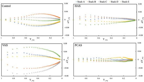
Figure 8.
Plots of of five stacks versus for four models during the entire cooling process. The x-axis indicates the average instantaneous temperature change fraction of all produce, and the y-axis stands for the means of differences between the instantaneous temperature change fraction of produce on each stack and the average temperature change fraction of all produce.
The instantaneous value of 15 rows was subtracted from the overall average value (denoted as ) to further analyze the uniformity of cooling across different stacks of produce. We then computed the mean value of these differences for each stack, represented as , at specific timestamps. The variation of relative to during the cooling process was subsequently examined across five stacks within each air supply system, as illustrated in Figure 7.
As the cooling process progressed, all four models displayed converging values across all five stacks, while the dynamics of temperature change with the same stack varied strongly between different models (Figure 8). In general, the VAS model exhibited the greatest heterogeneity among all models, whereas the PCAS model presented the most uniform behavior, with values ranging between −0.01 and 0.01. Following the PCAS model, the HAS model demonstrated the second-best uniformity across the stacks. Interestingly, the control model’s fastest cooling stack was Stack A, while Stack B was the slowest. Under the HAS scheme, Stack E cooled the fastest, with Stack C being the slowest. Contrary to the HAS model results, the VAS model’s fastest cooling stack was Stack C, and the slowest was Stack E. The PCAS model initially showed the fastest cooling in Stack D, until Stack B overtook it midway during the cooling process. However, towards the end, Stack E became the fastest, while Stack D replaced Stack A as the slowest stack (Figure 8).
Similarly, the heterogeneity of temperature change among produce at different heights was characterized by analyzing the instantaneous value of three levels over (Figure 8). Three levels, namely, Level 1, Level 2, and Level 3, denote increasing heights. For each level, data from five rows of produce were used to calculate the corresponding .
Generally, three of the four models exhibited a more uniform cooling performance across three levels compared to the five stacks, particularly for the VAS model (Figure 9). The PCAS model displayed the widest range of values from −0.04 to 0.04, with the fastest cooling observed at Level 3 (the highest). In contrast, the HAS model showed the most uniform cooling behavior across the three heights, with values ranging between −0.01 and 0.01, approximately. The fastest cooling in the HAS model was detected at Level 1, while the produce at Level 3 cooled slightly slower than Level 2. The control model’s results suggested that the produce at the lowest level cooled the fastest, with the slowest cooling observed at the middle level, which was similar to the observations in the VAS and PCAS results. Both models showed the slowest cooling performance at Level 2 among the three levels.
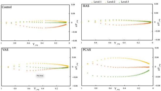
Figure 9.
Plots of of three levels versus for four models during the entire cooling process. The x-axis indicates the average instantaneous temperature change fraction of all produce, and the y-axis stands for the means of differences between the instantaneous temperature change fraction of produce on each level and the average temperature change fraction of all produce.
Additionally, the cooling uniformity at different locations of the room under each air supply scheme was analyzed by visualizing the indoor temperature distribution. Indoor temperature contours were created at 6, 12, 24, and 48 h of precooling to compare the temperature distribution between each row of Chinese cabbages at three selected cross-sectional planes (Figure 10, Figure 11 and Figure 12).
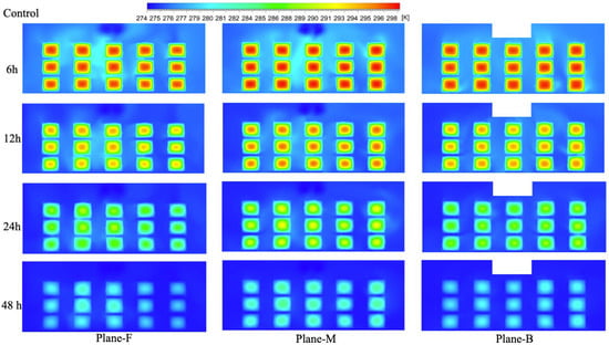
Figure 10.
Temperature contours at three selected planes for the control model. Each row represents temperature contours at 6, 12, 24, and 48 h of precooling. Contours within the same column belong to the same plane, as indicated at the bottom.
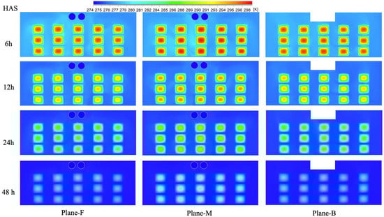
Figure 11.
Temperature contours at three selected planes for the HAS model. Each row represents temperature contours at 6, 12, 24, and 48 h of precooling. Contours within the same column belong to the same plane.
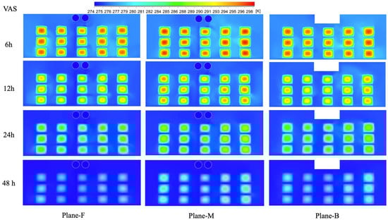
Figure 12.
Temperature contours at three selected planes for the VAS model. Each row represents temperature contours at 6, 12, 24, and 48 h of precooling. Contours within the same column belong to the same plane.
For the control model, the cooling of produce at Plane-B commenced relatively slower compared to the other two locations after 6 h of cooling (Figure 10). Although the ambient air temperature at Plane-B was lower than the others at the 6th hour of precooling, particularly at both middle aisles, noticeable light blue areas were visualized at Plane-F and Plane-M. However, the decrease in produce temperatures at Plane-M appeared to be the slowest one at 12, 24, and 48 h of precooling, suggesting that the field heat was more difficult to remove for produce at Plane-M compared to the other two locations. By the end of 48 h of precooling, temperatures of produce at Plane-F and Plane-B dropped roughly to 7 °C and below, with some boxes of produce nearing the target cooling temperature at certain rows. At Plane-F, produce in stacks B and C exhibited higher temperatures than the other stacks, although such an obvious difference was not observed at Plane-M and Plane-B.
The indoor temperature distribution of the HAS model showed strong symmetry (Figure 11), with the temperature of produce at Plane-F and Plane-B expressing almost identical patterns at all timestamps. However, it took longer to cool down the produce on Plane-M than on the other planes. Based on the temperature contours at the 48th hour of cooling, most of the outer portions inside each box at Plane-F and Plane-B blended into the background and became invisible as the temperature reached the target. At Plane-M, there were still some light blue areas, indicating that the produce required additional cooling time. One note is that the ambient air under the HAS scheme exhibited an almost evenly distributed temperature regardless of location at each contour.
The other air-ducting system, VAS, displayed a distinct pattern of temperature distribution compared to HAS (Figure 12). The temperature of the produce showed a consistent trend despite the cooling time: the produce at Plane-F cooled down the fastest, followed by those at Plane-B, while Plane-M was the slowest to cool down. The variations in temperature distributions between the three planes were not substantial. Moreover, the produce on Stack C constantly possessed the lowest temperature since cooling air was directly injected above it. Additionally, the temperature distribution of the ambient air at the 6th and 12th hour under the VAS scheme was slightly less uniform than that of the HAS model but was still more even compared to the control model.
A pattern similar to the VAS model was observed in the PCAS model in terms of having a faster cooling performance at Plane-F among the three selected planes at all timestamps, with the produce at Plane-B displaying a slightly lower temperature than Plane-M in general (Figure 13). Moreover, the produce at the same plane indicated excellent temperature uniformity, regardless of the locations. The temperature distribution of the ambient air at Plane-F and Plane-M was not able to provide comparable uniformity as models HAS or VAS presented, particularly at the 6th and 12th hours of cooling. However, the target cooling temperature was consistently maintained in the attic area under the PCAS scheme at all timestamps.
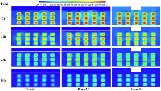
Figure 13.
Temperature contours at three selected planes for the PCAS model. Each row represents temperature contours at 6, 12, 24, and 48 h of precooling. Contours within the same column belong to the same plane, as indicated.
3.3. Airflow Patterns under Four Air Supply Systems
Four air supply schemes presented varying cooling effectiveness based on the comparison of temperature contours at critical timestamps. This comparison provided valuable insights into the relationship between these differences and the indoor airflow patterns within each system. Air velocity contours on selected planes were created using data from a 96 h simulation for each model to facilitate a visual comparison of the airflows (Figure 14, Figure 15 and Figure 16).
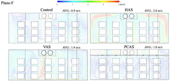
Figure 14.
Indoor air velocity contours Plane-F (the front cross-section of produce) from a 96-h simulation for each model. A legend of colors ranging from 0 to 5 m/s illustrates the magnitude of the air velocity. The average air speed is displayed upright for each contour. Note that velocities exceeding 5 m/s are represented in red.
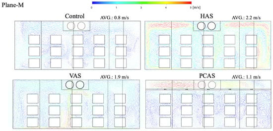
Figure 15.
Indoor air velocity contours Plane-M (the middle cross-section of produce) from a 96-h simulation for each model. A legend of colors ranging from 0 to 5 m/s illustrates the magnitude of the air velocity. The average air speed is displayed upright for each contour. Note that velocities exceeding 5 m/s are represented in red.
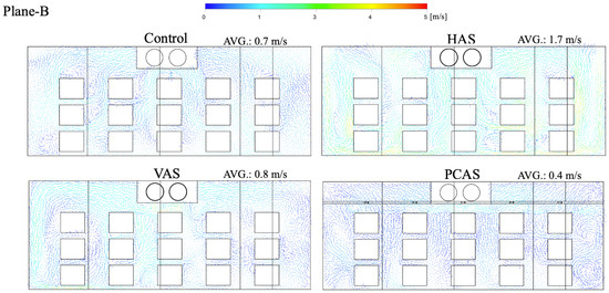
Figure 16.
Indoor air velocity contours Plane-F (the back cross-section of produce) from a 96-h simulation for each model. A legend of colors ranging from 0 to 5 m/s illustrates the magnitude of the air velocity. The average air speed is displayed upright for each contour. Note that velocities exceeding 5 m/s are represented in red.
At Plane-F, the control model revealed a general airflow pattern where air movement was predominantly from top to bottom. Intense airflows were detected moving from the upper right towards the central aisle between stacks C and D, with speeds around 1 m/s. Vertical airflows of significant magnitude were observed descending to the ground on both sides of the room. Note that upward airflows were also detected near the ground, particularly on the left side of the room and in the aisles between stacks A and B and stacks D and E. These upward airflows then encountered nearby downward airflows, resulting in the formation of some swirls at these locations (Figure 14). At Plane-M, additional swirls were observed in the aisles between stacks, as well as in areas close to both sides of the room (Figure 15). Substantial air velocities were observed traveling along the positive z-axis on the right side of Plane-M, as indicated by small arrowheads, creating a relatively blank area compared to the contour at Plane-F. The airflow patterns appeared more refined and generally shifted to an upward orientation at Plane-B (Figure 16). Numerous air velocities close to the upper-middle region were directed towards the outlet. Only a few small swirls with slow speeds were observed. Moreover, the average air speed of the three planes for the control model was very similar to each other.
The airflow patterns of the HAS model displayed lucid air movement paths with remarkable symmetry, especially at Plane-F and Plane-M (Figure 14, Figure 15 and Figure 16). The incoming cooling air from the air ducts formed robust injection air streams that traveled to both sidewalls along the ceiling in a flat trajectory. Upon hitting the sidewall, most of the airflows turned downward until they reached the floor at the corner, then penetrated underneath the boxes of produce towards the center of the room without losing much of their magnitude. Within each aisle between stacks, airflows ascended and utilized the space between boxes and upper spaces to form air circulations. Thus, symmetrical air circulation was generally noticed on both sides of the cold storage room for the HAS model. Additionally, strong air moments with some speeds exceeding 3 m/s around boxes were depicted in the contours on all three planes. The difference between airflows at Plane-F and Plane-M could be the influence of incoming cooling air, as the trajectory of injecting air was more rigorous and extensive at Plane-F than at Plane-M. However, stronger air circulations were detected at two middle aisles and the very right aisle between Stack E and the sidewall at Plane-M, which may be more beneficial for field heat removal. In fact, the average air speed of Plane-M was slightly higher than that of Plane-F. At Plane-B, the airflow patterns under HAS tended to vary, with symmetry still existing in terms of indoor air movement paths, although it may not be as clear as that observed from Plane-F or Plane-M (Figure 14, Figure 15 and Figure 16). In addition, the air speed decreased by 15% and 22.7% on average compared to Plane-F and Plane-M, respectively. Two noticeable air circulations were visualized near both sidewalls. Moreover, due to the influence of the outlet, most upward airflows on the right side moved towards the middle, although some air circulations were formed close to the ceiling on the left side.
Unlike the nearly symmetrical air movement paths of the HAS model, the VAS model presented distinct airflow patterns based on its simulation results. Since the cooling air was introduced vertically through air ducts, airflow initially traveled downward from both ducts at high speeds. The cooling air from the left air duct was able to maintain a long trajectory until it hit the ground at a high speed of up to 5 m/s and above, then proceeded underneath boxes to both sides (Figure 14, Figure 15 and Figure 16). However, the cooling air injected from the air duct on the right-side air duct directly impinged on the top boxes of Stack C, then rebounded and dispersed in various directions. At Plane-F, most of the right-side incoming air was deflected back and ascended towards the ceiling, partially lifted by the upward airflow from the bottom. Meanwhile, at Plane-M, the incoming air from the right side circled back to the middle right after hitting the boxes, merging with the drifts of horizontal airflows from right to left at the upper portion of the room (Figure 15). As a result, the produce on Stack C received considerable airflow around them, particularly those at the top level. The average air speed was the same at 1.9 m/s for both Plane-F and Plane-B, yet it decreased to 0.8 m/s on Plane-B. Indoor air generally exhibited less vigorous movement at Plane-B for VAS, although some upward airflows along the left sidewall were conspicuous with relatively fast speeds and became more pronounced approaching the outlet area (Figure 16). Note that the aisle between Stacks B and C possessed far more robust airflows than the others. Spaces between boxes in the right portion of the cold room showed stagnant air movement compared to the left portion. Also, some airflows moving along the -axis were observed at the right portion.
Due to the presence of an enclosed attic area housing the incoming cooling air, the PCAS model exhibited unique airflow patterns compared to the other three models. Vigorous air movements were observed inside the attic at both Plane-F and Plane-M, though the airflow patterns varied, with more cross-traveling airflows at the middle cross-section of the room compared to the front. The average air speed was similar for Plane-F and Plane-M, which was approximately 1 m/s. However, the space underneath the perforated ceiling showed relatively stagnant air movements (Figure 14, Figure 15 and Figure 16). Air velocities above 1 m/s were scarcely observed at the three selected planes, with most detected either near the ceiling or the ground. In addition, several swirls were noted between stacks of produce at Plane-F and Plane-M, yet not at Plane-B. In fact, based on the air velocity contours of the simulation results from PCAS, Plane-B possessed the least active air movements among the three planes, with an average air speed of 0.4 m/s. All those findings suggested a relatively weaker indoor air movement and unsustainable cooling efficacy under the PCAS scheme compared to the others, which could be the reason why the PCAS model possessed the lowest cooling rate in general.
4. Discussion
The air supply system of the HAS model demonstrated superior precooling performance compared to the others according to simulation output, presenting the most promising energy sustainability. The HCT of the HAS model is approximately 16 h, which is 4 h less than the control model. Furthermore, by using the HAS air supply scheme, about 12 h can be saved in terms of SECT compared to the control model, which equals a reduction of 18.8%. Although the VAS model shows a similar HCT to the HAS model, its SECT is around 58 h, which is still 6 h more than the HAS model. Hence, by using the HAS and VAS systems instead of the control type, the operating time could be reduced by about 12 and 6 h, respectively, to achieve the 7/8 target cooling temperature with the same evaporator unit, which can be a significant improvement in energy savings. However, the PCAS displayed a slower overall cooling time compared to the control model, with a similar HCT yet a 4 h delayed SECT.
Our combined analysis of airflow patterns and temperature distribution underscores the significant role that air supply systems play in precooling performance. A vigorous and well-organized airflow pattern has been demonstrated to enhance cooling efficacy and uniformity, as evidenced by the simulation results of the four models. Airflows in the HAS model generally present a symmetrical movement pattern, with robust air movements in open spaces, forming effective air circulations to remove field heat from produce (Figure 14, Figure 15 and Figure 16). Given that most airflows travel consistently and are well organized, a few unnecessary and adverse swirls are generated because of the confrontation of opposing airflows. In addition, it is critical to introduce cooling air horizontally in both directions, as in the HAS model, to fully utilize the width of the storage room. This allows high-speed incoming air to obtain sufficient space to develop a complete trajectory that maintains its momentum, rather than being deflected by obstacles or blocked by walls at an early stage. A complete air trajectory can maintain a consistent movement orientation as much as possible without losing the magnitude of air velocity.
Conversely, based on the layout of the cold storage room, a short distance between the front and back forced the incoming air from the evaporator to directly hit the front wall in the control model. The air speeds of the incoming cold air reduce considerably after hitting the front wall, then disperse in random order, mixing with the indoor warm air. As a result, more chaotic air movements were observed in the cross-sectional air velocity contours from the control model (Figure 14, Figure 15 and Figure 16). The slow cooling of produce at Plane-M and the central stacks of the control model (Figure 10) suggest that it is challenging for the cooling air to penetrate the space between the produce with slow and weak airflows. As previously reported, under these regular air supply schemes, some of the incoming cooling airflows may not be capable of developing paths to travel across stacks of produce before being exhausted from the outlet due to the misplacement of the location of inlets and outlets [17,47].
The airflow in the VAS model encounters a similar issue to the control model, as the incoming airstream from the right air duct is severely deflected by the produce. Consequently, the air movement on the right side is not as organized as on the left side (Figure 14, Figure 15 and Figure 16), which display small swirls and a number of tiny cross-traveling air velocities. Although the strong injection of cooling air from the left air duct promotes a robust descending airstream down to the ground before splitting in both directions, the air speeds on the right side are generally slower than those on the left. Another critical issue for the VAS model is the inefficient path of air movement. Most of its strong and consistent air movements are nearing the sidewall, while the airflows circulating around the produce are slower and less uniform compared to the HAS model, except for the two stacks beneath the left air duct. As a result, the primary challenge for the VAS system is the lack of cooling uniformity.
The PCAS model has not exhibited as competitive a cooling performance as the other two alternative systems and has even been outperformed by the control model. This is attributed to a significant lack of robust air movements around the produce. Although the perforated ceiling is capable of providing top-to-bottom airflows in a relatively uniform manner, as previously investigated, the corresponding cooling rate and cooling time have not been assessed [25,48]. According to our results, the cooling rate of the PCAS model is not optimal for precooling purposes. While the incoming air from the evaporator provides fast air speeds inside the attic, most of these speeds cannot be maintained when traveling through the vertical holes to the lower area. In addition, the indoor air movement of the PCAS model is spotty, with a few small swirls formed, which also hinders the cooling performance compared to the other models (Figure 14, Figure 15 and Figure 16). However, the PCAS model does have merits in cooling uniformity, particularly for the produce at the same level across stacks (Figure 13), which surpasses the other air supply systems.
All our findings demonstrate that CFD modeling is a powerful tool to investigate the refinement of air supply systems and examine the indoor environment via pertinent simulations. Further research may focus on optimizing these air supply systems by leveraging their airflow features and integrating other factors, such as the arrangement of produce and the layout of the storage room. In this study, the HAS model showed the most competitive cooling performance due to its relatively uniform airflows that effectively covered most of the space. Within the HAS scheme, the produce can be placed in a manner that may not coincide with the airflows.
However, the placement of produce should take the indoor airflow patterns into account due to the heterogeneity of cooling. For example, within the VAS model, the central region is supposed to cool more rapidly than other parts of the storage. Hence, making use of this disparity may also be worth investigating in practical applications, as some previous research has claimed that an unevenly distributed climate may have advantageous effects for certain specific applications [17].
Various air supply systems may be utilized in some specific scenarios. Herein, the PCAS scheme might not be ideal for forced-air precooling, but it can still be used for long-term cold storage after the produce has already been cooled down due to its steady and accountable cooling uniformity. Also, the PCAS model is the only scheme that shows faster cooling at a high level among the four models. In addition, the relatively low air speeds provided by the PCAS model may be more energy-sustainable, reducing the weight loss of some produce during long-term storage.
5. Conclusions
In conclusion, out of three alternative air supply systems, HAS and VAS demonstrated competitive precooling performances. Our analysis revealed that the HAS model’s SECT decreased by 18.8% and its maximum cooling rate rose by 19.7% in comparison to the control model. The VAS model’s SECT was 9.4% lower than the control model, and its maximum cooling rate increased by 10.5%.
Four models displayed varying degrees of cooling heterogeneity due to their unique air movement patterns. The HAS model exhibited the best overall cooling uniformity, attributed to its well-organized airflows. The VAS model displayed exceptionally robust cooling performances in the center region of the storage room.
Although the PCAS model presented the best cooling uniformity across five stacks, it possessed the highest cooling heterogeneity at different heights among all models. Furthermore, the maximum cooling rate of the PCAS model was 6.6% less than the control model, leading to a 6.3% longer SECT. This indicates that the precooling performance under the PCAS scheme may not be as effective as the others, and it was even slightly outperformed by the control model.
Supplementary Materials
The following supporting information can be downloaded at: https://www.mdpi.com/article/10.3390/su16083119/s1, Figure S1: Computational domain of the CFD model for validation; Table S1: GCI values calculated by corresponding mesh refinement ratios using the second-order scheme; Table S2: Field measurement versus prediction data at 16 locations.
Author Contributions
Conceptualization, L.C. and J.L.; methodology, L.C.; software, L.C.; validation, L.C. and W.W.; formal analysis, L.C.; investigation, L.C.; resources, Z.Z.; data curation, L.C.; writing—original draft preparation, L.C.; writing—review and editing, L.C.; visualization, L.C.; supervision, J.L. and Z.Z.; project administration, J.L.; funding acquisition, L.C. All authors have read and agreed to the published version of the manuscript.
Funding
This research was funded by the Key Laboratory of Storage of Agricultural Products, Ministry of Agriculture and Rural Affairs, China (Grant No. Kf2021009).
Institutional Review Board Statement
Not applicable.
Data Availability Statement
Data are contained within the article.
Acknowledgments
The authors acknowledge Tianjin Technology of Mushroom Engineering Center for the support of equipment and instruments to conduct this study.
Conflicts of Interest
The authors declare no conflicts of interest.
References
- FAO. Energy-Smart Food for People and Climate; FAO: Rome, Italy, 2011; p. 66. [Google Scholar]
- Duan, Y.; Wang, G.B.; Fawole, O.A.; Verboven, P.; Zhang, X.R.; Wu, D.; Opara, U.L.; Nicolai, B.; Chen, K. Postharvest precooling of fruit and vegetables: A review. Trends Food Sci. Technol. 2020, 100, 278–291. [Google Scholar] [CrossRef]
- Brosnan, T.; Sun, D.W. Precooling techniques and applications for horticultural products—A review. Int. J. Refrig. 2001, 24, 154–170. [Google Scholar] [CrossRef]
- Zhao, C.J.; Han, J.W.; Yang, X.T.; Qian, J.P.; Fan, B.L. A review of computational fluid dynamics for forced-air cooling process. Appl. Energy 2016, 168, 314–331. [Google Scholar] [CrossRef]
- Wang, D.; Lai, Y.; Jia, B.; Chen, R.; Hui, X.; Duan, Y.; Wang, G.B.; Fawole, O.A.; Verboven, P.; Zhang, X.R.; et al. The optimal design and energy consumption analysis of forced air pre-cooling packaging system. Appl. Therm. Eng. 2020, 165, 278–291. [Google Scholar] [CrossRef]
- Han, J.W.; Zhao, C.J.; Yang, X.T.; Qian, J.P.; Fan, B.L. Computational modeling of airflow and heat transfer in a vented box during cooling: Optimal package design. Appl. Therm. Eng. 2015, 91, 883–893. [Google Scholar] [CrossRef]
- Wang, G.; Zhang, X. Evaluation and optimization of air-based precooling for higher postharvest quality: Literature review and interdisciplinary perspective. Food Qual. Saf. 2020, 4, 59–68. [Google Scholar] [CrossRef]
- Delele, M.A.; Tijskens, E.; Atalay, Y.T.; Ho, Q.T.; Ramon, H.; Nicolaï, B.M.; Verboven, P. Combined discrete element and CFD modelling of airflow through random stacking of horticultural products in vented boxes. J. Food Eng. 2008, 89, 33–41. [Google Scholar] [CrossRef]
- Cao, Y.; Gong, Y.F.; Zhang, X.R. Impact of ventilation design on the precooling effectiveness of horticultural produce-a review. Food Qual. Saf. 2020, 4, 29–40. [Google Scholar] [CrossRef]
- Liu, X.; Nan, X. Improvement on characteristics of air flow field in cold storage with uniform air supply duct. Trans. Chin. Soc. Agric. Eng. 2016, 32, 91–96. (In Chinese) [Google Scholar]
- Chourasia, M.K.; Goswami, T.K. Three dimensional modeling on airflow, heat and mass transfer in partially impermeable enclosure containing agricultural produce during natural convective cooling. Energy Convers. Manag. 2007, 48, 2136–2149. [Google Scholar] [CrossRef]
- Mirade, P.S.; Kondjoyan, A.; Daudin, J.D. Three-dimensional CFD calculations for designing large food chillerq s. Comput. Electron. Agric. 2002, 34, 67–88. [Google Scholar] [CrossRef]
- Mulobe, N.J.; Huan, Z. Energy efficient technologies and energy saving potential for cold rooms. In Proceedings of the 2012 Proceedings of the 9th Industrial and Commercial Use of Energy Conference, Cape Town, South Africa, 15–16 August 2012; pp. 157–163. [Google Scholar]
- Praeger, U.; Jedermann, R.; Sellwig, M.; Neuwald, D.A.; Hartgenbusch, N.; Borysov, M.; Truppel, I.; Scaar, H.; Geyer, M. Airflow distribution in an apple storage room. J. Food Eng. 2020, 269, 109746. [Google Scholar] [CrossRef]
- Ghiloufi, Z.; Khir, T. CFD modeling and optimization of pre-cooling conditions in a cold room located in the South of Tunisia and filled with dates. J. Food Sci. Technol. 2019, 56, 3668–3676. [Google Scholar] [CrossRef]
- Mostafa, E.; Lee, I.B.; Song, S.H.; Kwon, K.S.; Seo, I.H.; Hong, S.W.; Hwang, H.S.; Bitog, J.P.; Han, H.T. Computational fluid dynamics simulation of air temperature distribution inside broiler building fitted with duct ventilation system. Biosyst. Eng. 2012, 112, 293–303. [Google Scholar] [CrossRef]
- Parpas, D.; Amaris, C.; Tassou, S.A. Investigation into air distribution systems and thermal environment control in chilled food processing facilities. Int. J. Refrig. 2018, 87, 47–64. [Google Scholar] [CrossRef]
- Wang, X.F.; Fan, Z.Y.; Li, B.G.; Liu, E.H. Variable air supply velocity of forced-air precooling of iceberg lettuces: Optimal cooling strategies. Appl. Therm. Eng. 2021, 187, 116484. [Google Scholar] [CrossRef]
- Wells, C.M.; Amos, N.D. Design of air distribution systems for closed greenhouses. In Acta Horticulturae 361: International Symposium on New Cultivation Systems in Greenhouse; ISHS: Leuven, Belgium, 1994; pp. 93–104. [Google Scholar]
- Weigand, B.; Spring, S. Multiple Jet Impingement—A Review. In TURBINE-09. Proceedings of International Symposium on Heat Transfer in Gas Turbine Systems; Begel House Inc.: Danbury, CT, USA, 2011; pp. 1–36. [Google Scholar]
- Xie, L.N.; Wang, C.Y.; Ding, L.Y.; Gui, Z.Y.; Zhang, L.; Shi, Z.X.; Li, B.; Chuntao, J. Heat stress alleviation for dairy cows housed in an open-sided barn by cooling fan and perforated air ducting (PAD) system. Int. J. Agric. Biol. Eng. 2017, 10, 1–10. [Google Scholar] [CrossRef]
- Wu, C.; Cheng, R.; Fang, H.; Yang, Q.; Zhang, C. Simulation and optimization of air tube ventilation in plant factory based on CFD. J. China Agric. Univ. 2021, 26, 78–87. (In Chinese) [Google Scholar]
- Gladyszewska-Fiedoruk, K.; Demianiuk, A.B.; Gajewski, A.; Olow, A. Measurement of velocity distribution for air flow through perforated plastic foil ducts. Energy Build. 2011, 43, 374–378. [Google Scholar] [CrossRef]
- Parpas, D.; Amaris, C.; Tassou, S.A. Experimental investigation and modelling of thermal environment control of air distribution systems for chilled food manufacturing facilities. Appl. Therm. Eng. 2017, 127, 1326–1339. [Google Scholar] [CrossRef]
- Guo, Y.; Liu, B.; Shen, S. Study on pre-cooling of fruit and vegetable in mini-cold storage. J. Therm. Sci. Technol. 2005, 4, 118–121. (In Chinese) [Google Scholar]
- Norton, T.; Sun, D.-W.; Grant, J.; Fallon, R.; Dodd, V. Applications of computational fluid dynamics (CFD) in the modelling and design of ventilation systems in the agricultural industry: A review. Bioresour. Technol. 2007, 98, 2386–2414. [Google Scholar] [CrossRef]
- Li, Y.; Nielsen, P.V. Commemorating 20 years of Indoor Air: CFD and ventilation research. Indoor Air 2011, 21, 442–453. [Google Scholar] [CrossRef] [PubMed]
- Hoang, M.L.; Verboven, P.; De Baerdemaeker, J.; Nicolaï, B.M. Analysis of the air flow in a cold store by means of computational fluid dynamics. Int. J. Refrig. 2000, 23, 127–140. [Google Scholar] [CrossRef]
- Nahor, H.B.; Hoang, M.L.; Verboven, P.; Baelmans, M.; Nicolaï, B.M. CFD model of the airflow, heat and mass transfer in cool stores. Int. J. Refrig. 2005, 28, 368–380. [Google Scholar] [CrossRef]
- Moureh, J.; Tapsoba, M.; Flick, D. Airflow in a slot-ventilated enclosure partially filled with porous boxes: Part I—Measurements and simulations in the clear region. Comput. Fluids 2009, 38, 194–205. [Google Scholar] [CrossRef]
- Moureh, J.; Tapsoba, M.; Flick, D. Airflow in a slot-ventilated enclosure partially filled with porous boxes: Part II—Measurements and simulations within porous boxes. Comput. Fluids 2009, 38, 206–220. [Google Scholar] [CrossRef]
- Shen, J.; Liu, X.; Wang, X.; Qi, H. Numerical simulation on flow field in jacketed ice—Temperature storage. Refrigeration 2009, 37, 49–53, 57. [Google Scholar]
- Moureh, J.; Flick, D. Airflow pattern and temperature distribution in a typical refrigerated truck configuration loaded with pallets. Int. J. Refrig. 2004, 27, 464–474. [Google Scholar] [CrossRef]
- Moureh, J.; Tapsoba, S.; Derens, E.; Flick, D. Air velocity characteristics within vented pallets loaded in a refrigerated vehicle with and without air ducts. Int. J. Refrig. 2009, 32, 220–234. [Google Scholar] [CrossRef]
- Zhang, Y.; Kacira, M.; An, L. A CFD study on improving air flow uniformity in indoor plant factory system. Biosyst. Eng. 2016, 147, 193–205. [Google Scholar] [CrossRef]
- ANSYS. User Guide; Release 12; ANSYS: Lebanon, NH, USA, 2009. [Google Scholar]
- Kim, J.-B.; Lee, D.-S.; Choin, D.-W.; Pyun, Y.-R. Thermal Conductivity of Petiole Tissue of Chinese Cabbage. Korean J. Food Sci. Technol. 1991, 23, 325–329. [Google Scholar]
- Becker, B.R.; Misra, A.; Fricke, B.A. Bulk refrigeration of fruits and vegetables part I: Theoretical considerations of heat and mass transfer. HVAC R Res. 1996, 2, 122–134. [Google Scholar] [CrossRef]
- WFLO. WFLO Commodity Storage Manual Cabbage; WFLO: Farmville, VA, USA, 2018. [Google Scholar]
- Roache, P.J. Perspective: A method for uniform reporting of grid refinement studies. J. Fluids Eng. Trans. ASME 1994, 116, 405–413. [Google Scholar] [CrossRef]
- Launder, B.E.; Spalding, D.B. The numerical computation of turbulent flows. Comput. Methods Appl. Mech. Eng. 1974, 3, 269–289. [Google Scholar] [CrossRef]
- Thompson, J.F.; Mitchell, F.G.; Rumsey, R.T.; Kasmire, R.F.; Crisosto, C.H. Commercial Cooling of Fruits, Vegetables, and Flowers, Revised ed.; Regents of the University of California: Oakland, CA, USA, 2008. [Google Scholar]
- Dehghannya, J.; Ngadi, M.; Vigneault, C. Mathematical modeling of airflow and heat transfer during forced convection cooling of produce considering various package vent areas. Food Control 2011, 22, 1393–1399. [Google Scholar] [CrossRef]
- Chang, J.C.; Hanna, S.R. Air quality model performance evaluation. Meteorol. Atmos. Phys. 2004, 87, 167–196. [Google Scholar] [CrossRef]
- Tong, X.; Hong, S.W.; Zhao, L. CFD modelling of airflow pattern and thermal environment in a commercial manure-belt layer house with tunnel ventilation. Biosyst. Eng. 2019, 178, 275–293. [Google Scholar] [CrossRef]
- Küçüktopcu, E.; Cemek, B.; Simsek, H.; Ni, J.Q. Computational Fluid Dynamics Modeling of a Broiler House Microclimate in Summer and Winter. Animals 2022, 12, 867. [Google Scholar] [CrossRef]
- Parpas, D.; Amaris, C.; Sun, J.; Tsamos, K.M.; Tassou, S.A. Numerical study of air temperature distribution and refrigeration systems coupling for chilled food processing facilities. Energy Procedia 2017, 123, 156–163. [Google Scholar] [CrossRef]
- Liu, B.; Yang, Z.; Li, X.; Tan, J. Experiment on Air Distribution and Storage Effects. J. Tianjin Univ. 2005, 38, 897–900. [Google Scholar]
Disclaimer/Publisher’s Note: The statements, opinions and data contained in all publications are solely those of the individual author(s) and contributor(s) and not of MDPI and/or the editor(s). MDPI and/or the editor(s) disclaim responsibility for any injury to people or property resulting from any ideas, methods, instructions or products referred to in the content. |
© 2024 by the authors. Licensee MDPI, Basel, Switzerland. This article is an open access article distributed under the terms and conditions of the Creative Commons Attribution (CC BY) license (https://creativecommons.org/licenses/by/4.0/).