Tourism Transport-Related CO₂ Emissions and Economic Growth: A Deeper Perspective from Decomposing Driving Effects

Abstract

This study explores the intricate dynamics of CO₂ emissions stemming from transport within the tourism sector. It aims to unravel the multidimensional aspects of how transport-related tourism contributes to CO₂ emissions and to elucidate the complex relationship between regional economic growth and CO₂ emissions from transport-related tourism. Our study employed Logarithmic Mean Divisia Index (LMDI) and Panel Vector Autoregression (PVAR) models to analyze data from 30 Chinese provincial regions between 2010 and 2018. The tourism transport-related CO₂ emissions were decomposed into four separate driving effects using the LMDI approach. Then, PVAR models were constructed to reveal dynamic interactions between each driving effect and per capita gross regional product (GRP). Our results demonstrate a decrease in both energy structure effect (tourism transport-related CO₂ emissions from energy structure) and energy intensity effect (tourism transport-related CO₂ emissions from energy intensity) during the pre-COVID decade. Notably, the positive impulse response of energy structure effect to per capita GRP is observed. However, we found no evidence of a cointegrated relationship between energy intensity effect and regional economic growth, although other factors demonstrated connections. These findings echo the necessity to integrate sustainable practices into the tourism transportation business, especially in the area of energy structure, in order to mitigate adverse environmental effects from tourism. This paper disseminates the main drivers of CO₂ emissions in the tourism transport sector and their interrelationship with regional economic growth. It not only guides tourism policymakers in targeting efforts to reduce carbon footprints, but also sets a new benchmark for future studies on CO₂ emissions.

1. Introduction

Carbon dioxide (CO₂) emissions are a major driver of climate change, with significant implications for global environmental and socio-economic systems. The tourism industry is a notable contributor to global carbon emissions [1,2], accounting for approximately 8% of global greenhouse gas emissions [2,3]. These emissions arise from various sources within the tourism system, including transport, accommodation, and other activities [4,5,6]. According to the United Nations World Tourism Organization (UNWTO), transport plays a critical role in the tourism sector, being responsible for 75% of its carbon dioxide emissions [7]. Carbon dioxide emissions from transport, such as aviation and automobiles, are significant contributors to greenhouse gas emissions and have a substantial impact on global climate change [8]. Studying transport-related CO₂ emissions in tourism helps reveal the specific role of the tourism industry in climate change and provides effective measures to mitigate these emissions [9]. Moreover, compared to other sources of tourism carbon emissions, such as energy consumption in accommodation and attractions, research into transport-related CO₂ emissions is crucial for understanding the tourism industry’s specific role in climate change and for devising effective mitigation strategies. By studying transport-related carbon dioxide emissions in tourism, specific methods and strategies can be identified to reduce this type of emissions and lower the overall carbon emissions of the tourism industry [10].

Many researchers have studied how economic growth may influence transport CO₂ emissions inspired by the Environmental Kuznets Curve (EKC) hypothesis [11,12,13,14]. The tourism industry also constitutes a significant contributor to transport CO₂ emissions [8,9,10]. Using the Logarithmic Mean Divisia Index (LMDI) method [15,16,17], the changes in tourism transport-related CO₂ emissions could be decomposed to underlying driving effects. An inner driving effect is the change in CO₂ emissions caused by a specific inner driving factor [9]. This paper aims to examine the relationship between economic growth and tourism transport-related CO₂ emissions at a more in-depth level. Specifically, it aims to explore how economic growth affects each decomposing driving effect of tourism transport-related CO₂ emissions. Knowing the influence of economic growth on these driving effects is important. It can facilitate a better and deeper understanding of the mechanisms by which the economic growth could affect tourism transport-related CO₂ emissions. Then policymakers and industry stakeholders can develop relevant targeted interventions to reduce tourism CO₂ emissions and formulate policies for sustainable development in the tourism industry.

This paper tackles an important research void by investigating the deeper mechanisms by which economic growth influences tourism transport-related CO₂ emissions through innovative technical approaches. While the existing body of research provides some insights, there is a lack of comprehensive analysis using the methodologies of LMDI and panel vector autoregression (PVAR) models. This study aims to bridge this gap by employing these techniques. First, we will collect raw data from relevant Chinese yearbooks, official reports, etc. Then, we will calculate the elements that constitute CO₂ emissions from tourism transport. Next, the LMDI approach will be used to decompose CO₂ emissions into several important driving effects. Furthermore, this paper’s major contribution is marked by the application of LMDI and PVAR techniques, aiming to establish a connection between each driving effect of CO₂ emissions from tourism transport and economic growth indicators such as per capita gross regional product. Through the dissemination of driving effects, industry practitioners and policymakers can illuminate the intricate relationship that exists between carbon emissions and economic growth in the tourism transport sector. This will enable them to determine which elements of driving effects can be utilized as strategies to mitigate CO₂ emissions while determining which elements should be decelerating without compromising economic growth in the tourism industry, a fundamental tenant of sustainability.

The subsequent sections are organized as follows: Section 2 provides the literature review. Section 3 outlines the processing methods employed and describes the data utilized. Section 4 presents the results and engages in a discussion of the findings. Finally, the conclusions are articulated.

2. Literature Review

In typical assessments of CO₂ emissions from tourism transport, researchers focus on the mode of transport (air, rail, car, etc.) and calculate emissions based on passenger kilometers (pkm) for each mode [15,18]. Gunter et al. [8] introduced a method to evaluate CO₂ emissions from transportation in European city tourism, taking into account travel distance and transportation modes. Yang et al. [9] considered three transport modes, including train, road, and civil aviation, and then calculated the tourism traffic carbon emissions in Dunhuang, China. Safaa et al. [19] calculated the carbon footprint of travel to Marrakech, Morocco, based on the means of transportation and the distances traveled. A key aspect of these studies above involves establishing the CO₂ emission factors (kg/pkm) for each transport mode, assuming these emission factors remain constant over time. However, this assumption can lead to inaccuracies, as CO₂ emission factors change with shifts towards cleaner energy sources, like the transition from fuel-based to electric vehicles. This paper responds to this evolving landscape by employing a direct measurement technique for CO₂ emissions, focusing on fuel type and consumption. This approach not only tackles the fluctuating nature of emission factors but also ensures a more accurate measurement of CO₂ emissions, an important consideration in the context of rapidly changing transportation technologies. This approach is commonly used in other applications of CO₂ emissions [17,20,21], but is relatively rare in the context of tourism transport-related CO₂ emissions.

The Logarithmic Mean Divisia Index (LMDI) decomposition analysis is a widely used method to understand the driving effects behind changes in energy consumption or CO₂ emissions, notable for its capacity to fully eliminate the residual term, which guarantees a comprehensive factorization of effects [22]. This is in contrast to the conventional Laspeyres technique, which fails to achieve perfect decomposition and leaves a residual term [16]. This constraint is not only addressed by LMDI, but it also blends mathematical accuracy with the usefulness of typical index decomposition techniques [17]. Li [20] studied the factors that affected CO₂ emissions in China’s transportation sector using the LMDI model and the Cobb–Douglas production function. Chen et al. [23] examined carbon emissions from land use and applied LMDI to analyze the influencing factors in the area of northeast China. Gołaś [24] decomposed the changes in agricultural CO₂ emissions to six factors using LMDI in Polish agriculture. However, the application of LMDI to transport-related CO₂ emissions within the tourism sector has rarely been examined before. We intend to provide valuable insights into the underlying driving effects of transport-related CO₂ emissions in tourism.

The exploration of the relationship between economic growth and carbon emissions is becoming a hot research topic [11,25]. Many scholars have used the Tapio decoupling model to study this relationship [26,27,28]. However, the Tapio decoupling model is a non-parametric model, unable to accurately characterize the extent of the impact of economic growth on carbon emissions. In addition, some scholars have used traditional linear regression models to study the relationship between economic growth and carbon emissions [12,13,14]. However, traditional linear regression models have difficulties in distinguishing between endogenous and exogenous variables, as well as in handling lagged effects. The vector autoregression (VAR) model does not require explicit assumptions about the functional form. All variables are treated as endogenous, allowing for the analysis of the impact of each variable and its lagged effects on other variables [29]. The panel vector autoregression (PVAR) model is an extension of the traditional vector autoregression (VAR) model, incorporating the advantages of both panel data analysis and VAR modeling [30]. The advantages include: first, it fully accounts for individual fixed effects and time effects, ensuring better control of individual heterogeneity; second, the PVAR model effectively utilizes panel data, overcoming the requirement of long time series in the traditional VAR model [31]. Li et al. [32] examined the dynamic relationship between economic growth, CO₂ emissions and clean energy in China using the PVAR model. Jahanger et al. [33] utilized the PVAR method to analyze the influence of economic development, transportation, renewable energy, and globalization on the tourism sector and carbon emissions in the region around the Bay of Bengal. Zhang et al. [34] investigated the application of the PVAR model to analyze the relationship among economic growth, urbanization, energy consumption, and carbon emissions from 30 provinces in China. However, few studies have used the PVAR model to examine the decomposing driving effect of tourism transport CO₂ emissions.

Therefore, this study will choose the PVAR and LMDI techniques to investigate the impact of economic growth on each decomposing driving effect. It could reveal the deeper mechanisms by which economic growth affects tourism transport-related CO₂ emissions.

3. Materials and Methods

3.1. Measuring Transport-Related CO₂ Emissions in Tourism

The indicator used to characterize CO₂ emissions is tourism transport CO₂ emissions. In order to calculate tourism transport CO₂ emissions, the most commonly used method is to first calculate transport CO₂ emissions, and then separate the tourism-related part according to the tourism stripping coefficient [35,36,37]. This calculation employs the formula below:

$$C^{\left(i,t\right)}=s^{\left(i,t\right)}{\displaystyle \sum }_j\left(F_j^{\left(i,t\right)}{\alpha }_j{\beta }_j\right)$$

(1)

where $s^{\left(i,t\right)}$ is the tourism stripping coefficient [35]; F is the fuel consumption in the transport sector measured in the original physical unit; j is the fuel type; ${\alpha }_j$ is the conversion factor from physical unit to coal equivalent, as shown in

Table 1. Conversion factor to coal equivalent. (source China Energy Statistical Yearbook).

No.	Type	Factor	Unit
1	Raw coal	0.7143	kgCE/kg
2	Gasoline	1.4714	kgCE/kg
3	Kerosene	1.4714	kgCE/kg
4	Diesel	1.4571	kgCE/kg
5	Fuel oil	1.4286	kgCE/kg
6	Liquefied petroleum gas	1.7143	kgCE/kg
7	Natural gas	1.2150	kgCE/m3
8	Liquefied natural gas	1.7572	kgCE/kg
9	Heat	0.0341	kgCE/MJ
10	Electricity	0.1229	kgCE/(kW·h)

; ${\beta }_j$ stands for carbon dioxide emission factors, as shown in

Table 2. Carbon dioxide emission factors. (source 2006 IPCC Guidelines).

No.	Type	Factor	Unit
1	Raw coal	2.7724	kgCO2/kgCE
2	Gasoline	2.0310	kgCO2/kgCE
3	Kerosene	2.0955	kgCO2/kgCE
4	Diesel	2.1716	kgCO2/kgCE
5	Fuel oil	2.2684	kgCO2/kgCE
6	Liquefied petroleum gas	1.8493	kgCO2/kgCE
7	Natural gas	1.6441	kgCO2/kgCE
8	Liquefied natural gas	1.6441	kgCO2/kgCE
9	Heat	0.0000	kgCO2/kgCE
10	Electricity	0.0000	kgCO2/kgCE

.

3.2. LMDI

The Logarithmic Mean Divisia Index (LMDI) technique is a valuable method of assessing changing trends in carbon dioxide emissions [16]. By decomposing overall changes into individual driving effects, LMDI allows for a more detailed analysis of carbon dioxide emission changes [17]. Through decomposition, we gain insight into the individual contributions of different driving effects to carbon dioxide emissions, enabling targeted measures to be taken to reduce carbon dioxide emissions within the tourism industry [15,22].

The formula of the LMDI method can be derived from the Kaya identity [38]. The Kaya identity is a commonly used mathematical model to express carbon dioxide emissions, which decomposes carbon dioxide emissions into the product of four driving factors: energy structure effect, energy intensity effect, expenditure effect and scale effect.

The formula for Kaya identity [38] is given by:

$$C=\frac{C}{E}\cdot \frac{E}{G}\cdot \frac{G}{P}\cdot P$$

(2)

where C denotes transport-related CO₂ emissions in tourism, E denotes transport-related energy consumption emissions in tourism, G denotes earnings from tourism, P denotes number of tourists.

Let $x_1=C∕E$, $x_2=E∕G$, $x_3=G∕P$, $x_4=P$, then Equation (2) can be rewritten as:

$$C=x_1\cdot x_2\cdot x_3\cdot x_4$$

(3)

where $x_1, x_2, x_3,x_4$ are four driving factors, which are energy structure, energy intensity, expenditure and scale, respectively.

At a specific region i and time t₀, the CO₂ emissions are:

$$C^{\left(i,t_0\right)}={x_1}^{\left(i,t_0\right)}\cdot {x_2}^{\left(i,t_0\right)}\cdot {x_3}^{\left(i,t_0\right)}\cdot {x_4}^{\left(i,t_0\right)}$$

(4)

At a specific region i and time t, the CO₂ emissions are:

$$C^{\left(i,t\right)}={x_1}^{\left(i,t\right)}\cdot {x_2}^{\left(i,t\right)}\cdot {x_3}^{\left(i,t\right)}\cdot {x_4}^{\left(i,t\right)}$$

(5)

$D{C}^{\left(i,t\right)}$ denotes the change in CO₂ emissions from t₀ to t, which can be written as:

$$D{C}^{\left(i,t\right)}=C^{\left(i,t\right)}-C^{\left(i,t_0\right)}$$

(6)

Let $L^{\left(i,t\right)}=\frac{C^{\left(i,t\right)}-C^{\left(i,t_0\right)}}{\ln C^{\left(i,t\right)}-\ln C^{\left(i,t_0\right)}}$, then Equation (6) can be rewritten as:

$$\begin{gathered} D{C}^{\left(i,t\right)}=\frac{C^{\left(i,t\right)}-C^{\left(i,t_0\right)}}{\ln C^{\left(i,t\right)}-\ln C^{\left(i,t_0\right)}} \left(\ln C^{\left(i,t\right)}-\ln C^{\left(i,t_0\right)}\right) \\ =L^{\left(i,t\right)} \left[\ln \left( {x_1}^{\left(i,t\right)}\cdot {x_2}^{\left(i,t\right)}\cdot {x_3}^{\left(i,t\right)}\cdot {x_4}^{\left(i,t\right)}\right)-\ln \left({x_1}^{\left(i,t_0\right)}\cdot {x_2}^{\left(i,t_0\right)}\cdot {x_3}^{\left(i,t_0\right)}\cdot {x_4}^{\left(i,t_0\right)}\right)\right] \\ =L^{\left(i,t\right)} \left(\ln \frac{{x_1}^{\left(i,t\right)}}{{x_1}^{\left(i,t_0\right)}}+\ln \frac{{x_2}^{\left(i,t\right)}}{{x_2}^{\left(i,t_0\right)}}+\ln \frac{{x_3}^{\left(i,t\right)}}{{x_3}^{\left(i,t_0\right)}}+\ln \frac{{x_4}^{\left(i,t\right)}}{{x_4}^{\left(i,t_0\right)}}\right) \\ =L^{\left(i,t\right)}\ln \frac{{x_1}^{\left(i,t\right)}}{{x_1}^{\left(i,t_0\right)}}+L^{\left(i,t\right)}\ln \frac{{x_2}^{\left(i,t\right)}}{{x_2}^{\left(i,t_0\right)}}+L^{\left(i,t\right)}\ln \frac{{x_3}^{\left(i,t\right)}}{{x_3}^{\left(i,t_0\right)}}+L^{\left(i,t\right)}\ln \frac{{x_4}^{\left(i,t\right)}}{{x_4}^{\left(i,t_0\right)}} \\ =D{C}_{x_1}^{\left(i,t\right)}+D{C}_{x_2}^{\left(i,t\right)}+D{C}_{x_3}^{\left(i,t\right)}+D{C}_{x_4}^{\left(i,t\right)} \end{gathered}$$

(7)

where $D{C}_{x_1}, D{C}_{x_2}, D{C}_{x_3}, D{C}_{x_4}$ are four driving effects, which are defined as follows.

$D{C}_{x_1}^{\left(i,t\right)}=L^{\left(i,t\right)}\ln \frac{{x_1}^{\left(i,t\right)}}{{x_1}^{\left(i,t_0\right)}}$, represents energy structure effect;

$D{C}_{x_2}^{\left(i,t\right)}=L^{\left(i,t\right)}\ln \frac{{x_2}^{\left(i,t\right)}}{{x_2}^{\left(i,t_0\right)}}$, represents energy intensity effect;

$D{C}_{x_3}^{\left(i,t\right)}=L^{\left(i,t\right)}\ln \frac{{x_3}^{\left(i,t\right)}}{{x_3}^{\left(i,t_0\right)}}$, represents expenditure effect;

$D{C}_{x_4}^{\left(i,t\right)}=L^{\left(i,t\right)}\ln \frac{{x_4}^{\left(i,t\right)}}{{x_4}^{\left(i,t_0\right)}}$, represents scale effect.

Through the LMDI formula, the change in carbon dioxide emission could decompose into four driving effects. By assessing the relative importance of each driving effect, the targeted policy implications and suggestions can be provided. Definitions of the LMDI variables are summarized in

Table 3. Definitions of the LMDI variables.

Symbol	Variable	Indicator	Unit
$C$	CO2 emissions	Transport-related CO2 emissions in tourism	104 ton
$E$	Energy consumption	Transport-related energy consumption in tourism	104 tonCE
$G$	Gross economic output	Earnings from tourism	100 million CNY
$P$	Population	Number of tourist arrivals	104 person-times
$x_1$	Energy structure factor	Ratio of C to E	ton/tonCE
$x_2$	Energy intensity factor	Ratio of E to G	tonCE/104 CNY
$x_3$	Expenditure factor	Ratio of G to P	104 CNY/person
$x_4$	Scale factor	$P$	104 persons
$D{C}_{x_1}$	Energy structure effect	$L^{\left(i,t\right)} \ln \left({x_1}^{\left(i,t\right)}/{x_1}^{\left(i,t_0\right)}\right)$	104 ton
$D{C}_{x_2}$	Energy intensity effect	$L^{\left(i,t\right)} \ln \left({x_2}^{\left(i,t\right)}/{x_2}^{\left(i,t_0\right)}\right)$	104 ton
$D{C}_{x_3}$	Expenditure effect	$L^{\left(i,t\right)} \ln ({x_3}^{\left(i,t\right)}/{x_3}^{\left(i,t_0\right)}$)	104 ton
$D{C}_{x_4}$	Scale effect	$L^{\left(i,t\right)} \ln ({x_4}^{\left(i,t\right)}/{x_4}^{\left(i,t_0\right)}$)	104 ton

.

To facilitate a more comprehensive understanding of the LMDI approach, an in-depth description of each variable’s definition, measurement, and calculation procedures is provided below.

(1)

Energy consumption

The indicator we used here to characterize energy consumption is transport-related energy consumption in tourism, which is calculated using the following formula:

$$E^{\left(i,t\right)}=s^{\left(t\right)}{\displaystyle \sum }_j\left(F_j^{\left(i,t\right)}{\alpha }_j\right)$$

(8)

in the usual notation.

(2)

Gross economic output

The indicator we used here to characterize gross economic output is the earnings from tourism, including domestic tourism and international tourism. The values have been converted into 2010 prices using the consumer price index (CPI) [39].

(3)

Population

The indicator we chose to characterize the population is the number of tourist arrivals, including domestic and overseas tourists.

3.3. PVAR Model

In recent years, the panel vector autoregression (PVAR) model has been widely applied in economic research [32]. The PVAR model is an extension of the traditional vector autoregression (VAR) model, incorporating the advantages of both panel data analysis and VAR modeling [34]. The VAR model does not require the prior specification of causal relationships among variables [29]. Instead, all variables are treated as endogenous, allowing for the analysis of the impact of each variable and its lagged values on other variables within the model. This approach reduces the need for specific causal assumptions and enhances the flexibility and freedom of the model. Compared to the VAR model, the PVAR model has several distinctive advantages [40]. Firstly, it fully accounts for individual fixed effects and time effects, ensuring better control of individual heterogeneity. Secondly, the PVAR model effectively utilizes panel data, overcoming the requirement of long time series in the traditional VAR model. It is particularly useful when dealing with datasets that have a large cross-sectional dimension and relatively short time span.

The PVAR model in this paper focused on two variables: the driving effect of change in carbon dioxide emissions ($D{C}_{x_k}$) and per capita gross regional product (PG). Per capita gross regional product is a widely used indicator of economic growth [41,42]. The equation of the PVAR model can be given as follows:

$$\left[\begin{array}{c}D{C}_{x_k}^{\left(i,t\right)}\\ P{G}^{\left(i,t\right)}\end{array}\right]=A^{\left(0\right)}+A^{\left(1\right)}\left[\begin{array}{c}D{C}_{x_1}^{\left(i,t-1\right)}\\ P{G}^{\left(i,t-1\right)}\end{array}\right]+A^{\left(2\right)}\left[\begin{array}{c}D{C}_{x_1}^{\left(i,t-2\right)}\\ P{G}^{\left(i,t-2\right)}\end{array}\right]+\dots +A^{\left(n\right)}\left[\begin{array}{c}D{C}_{x_1}^{\left(i,t-n\right)}\\ P{G}^{\left(i,t-n\right)}\end{array}\right]+\left[\begin{array}{c}{\epsilon }_1\\ {\epsilon }_2\end{array}\right]$$

(9)

where i represents the region; t represents the time; k = 1, 2, 3, 4; ${\epsilon }_1$ and ${\epsilon }_2$ are the error terms; PG represents per capita gross regional product in CNY 10,000, which has been transformed into the 2010 price using the CPI [39]; $A^{\left(0\right)}$, $A^{\left(1\right)}$, …, $A^{\left(n\right)}$ denote the coefficient parameter matrices. The coefficient parameter matrices are defined below:

$$\begin{gathered} A^{\left(0\right)}=\left[\begin{array}{c}{a}_1^{\left(0\right)}\\ a_2^{\left(0\right)}\end{array}\right] \\ {A}^{\left(1\right)}=\left[\begin{array}{cc}{a}_{11}^{\left(1\right)}& a_{12}^{\left(1\right)}\\ a_{21}^{\left(1\right)}& a_{22}^{\left(1\right)}\end{array}\right] \\ {A}^{\left(2\right)}=\left[\begin{array}{cc}{a}_{11}^{\left(2\right)}& a_{12}^{\left(2\right)}\\ a_{21}^{\left(2\right)}& a_{22}^{\left(2\right)}\end{array}\right] \\ {A}^{\left(n\right)}=\left[\begin{array}{cc}{a}_{11}^{\left(n\right)}& a_{12}^{\left(n\right)}\\ a_{21}^{\left(n\right)}& a_{22}^{\left(n\right)}\end{array}\right] \end{gathered}$$

(10)

Generally, the key steps involved in the analysis of PVAR model are as follows:

• Panel variable stationarity test: Before applying PVAR model, it is important to test whether the data of each variable are stationary. This can be achieved using unit root tests such as the Im-Pesaran-Shin (IPS) test or Hadri LM test.
• Cointegration test: If two or more variables are found to be non-stationary, then it is necessary to test for cointegration among them. Cointegration implies a long-run relationship between the variables, and it is tested using methods such as the Pedroni test [40].
• Model order selection: Once the cointegration tests are complete, the next step is to determine the appropriate order of the PVAR model. This can be achieved using information criteria such as the Akaike information criterion (AIC), Bayesian information criterion (BIC), and Hannan–Quinn information criterion (HQIC).
• Parameter estimation: After selecting the appropriate order of the PVAR model, the next step is to estimate the parameters of the model. This can be achieved using the generalized method of moment (GMM).
• Impulse response function: The direction and magnitude of an impulse response are crucial to understanding the dynamic relationships between variables. Impulse response function could examine how a shock to one variable affects another variable over time and can help in identifying the direction and magnitude of the impact.

3.4. Technical Route

The technical route of this research can be summarized into the following steps:

• The raw data are obtained from relevant yearbooks, official reports, etc.;
• The raw data are then processed to calculate the driving factors;
• The LMDI method is then used to decompose the changes in carbon dioxide emissions;
• PVAR models are used to analyze the relationship between each driving effect and gross regional product per capita.

3.5. Data

This paper studied the tourism development in China. During the period from 2010 to 2018, China’s tourism industry experienced rapid development. According to data from the National Bureau of Statistics of China (http://www.stats.gov.cn/, accessed on 6 January 2024), the number of domestic tourists received nationwide increased from 2.27 billion in 2010 to 5.74 billion in 2018, an increase of 153%. At the same time, the number of inbound tourists increased from 13.59 million in 2010 to 30.69 million in 2018, an increase of 126%. The development of the tourism industry has made an increasingly significant contribution to China’s economy. The direct contribution of the tourism industry to gross domestic product (GDP) was CNY 1.38 trillion and accounted for 2.6% of GDP in 2010, while in 2018, the direct contribution of the tourism industry to GDP was CNY 5.97 trillion and accounted for 4.5% of GDP. The timeframe of 2010 to 2018 was chosen because it depicts a growth of China’s tourism industry of four times in size and an increasing contribution to the national economy. Furthermore, this period predates the disruptive effects of COVID-19 and related disease control policy on tourism, capturing the industry’s expansion phase in China. However, this rapid expansion also highlighted the negative environmental externalities.

China has 34 provincial-level administrative regions. This paper studied 30 provincial regions in view of the data availability. The other four regions, namely Xi Zang, Xiang Gang, Tai Wan and Ao Men, were not studied in this article because the data in these regions are partially missing. Figure 1 shows the position of these 30 provincial regions. According to data from the National Bureau of Statistics of China, the international tourism earnings of these 30 regions went from USD 51.87 billion in 2010 to USD 77.76 billion in 2018. At the same time, the gross regional product (GRP) of these 30 regions went from CNY 43.65 trillion in 2010 to CNY 91.32 trillion in 2018. The raw data for calculating CO₂ emissions and driving factors were collected from the China Statistical Yearbook, Yearbook of China Tourism Statistics, China Energy Statistical Yearbook, Statistical Yearbook of each province and relevant official reports. Some software (e.g., MATLAB R2019b, STATA 15) was also utilized in this experiment.

4. Results and Discussion

4.1. Transport-Related CO₂ Emissions in Tourism

According to the methods and raw data described in Section 3, the transport-related CO₂ emissions in tourism were calculated, along with their four driving factors.

Table 4. Carbon dioxide emissions and its driving factors.

Variables	Sample Size	Min	Max	Mean	Std. Dev	Unit
$C$	270	65.2891	4213.2916	1047.7088	716.7502	104 ton
$x_1$	270	1.7772	2.2669	2.0260	0.0869	ton/tonCE
$x_2$	270	0.0473	0.8204	0.2290	0.1387	tonCE/104 CNY
$x_3$	270	0.0428	0.8275	0.1031	0.0607	104 CNY/person
$x_4$	270	1020.6000	96,779.5744	30,675.5945	9223.3720	104 persons

reports the results of the transport-related carbon dioxide emissions in tourism and their influencing factors.

4.2. LMDI

In Equation (7), let $t_0=2010$. Then the change in transport-related CO₂ emissions in tourism could decompose every year. The results of driving effects are reported in

Table 5. Driving effects.

Variable	Symbol	Sample Size	Min	Max	Mean	Std. Dev	Unit
Energy structure effect	$D{C}_{x_1}$	240	−102.6507	87.8050	−12.8585	26.9944	104 ton
Energy intensity effect	$D{C}_{x_2}$	240	−1019.9881	1570.5697	53.9291	369.1905	104 ton
Expenditure effect	$D{C}_{x_3}$	240	−551.4894	1472.7198	45.5760	169.8453	104 ton
Scale effect	$D{C}_{x_4}$	240	−724.4963	2569.3748	513.4557	447.8619	104 ton

. From the table, it can be seen that $D{C}_{x_1}$ tends to be negative on average, while $D{C}_{x_2}$, $D{C}_{x_3}$ and $D{C}_{x_4}$ tend to be positive on average.

Table 6. Driving effects of the change in tourism transport CO₂ emissions.

Year	Energy Structure Effect		Energy Intensity Effect		Expenditure Effect		Scale Effect		Total Change
	${\mathsf{\Sigma }}_{\mathbf{i}}\mathit{D}{\mathit{C}}_{{\mathit{x}}_1}^{\left(\mathbf{i},\mathbf{t}\right)}$	Contribution	${\mathsf{\Sigma }}_{\mathbf{i}}\mathit{D}{\mathit{C}}_{{\mathit{x}}_2}^{\left(\mathbf{i},\mathbf{t}\right)}$	Contribution	${\mathsf{\Sigma }}_{\mathbf{i}}\mathit{D}{\mathit{C}}_{{\mathit{x}}_3}^{\left(\mathbf{i},\mathbf{t}\right)}$	Contribution	${\mathsf{\Sigma }}_{\mathbf{i}}\mathit{D}{\mathit{C}}_{{\mathit{x}}_4}^{\left(\mathbf{i},\mathbf{t}\right)}$	Contribution
2010–2011	−17.0439	−0.263%	3266.5335	50.368%	−74.1370	−1.143%	3309.9447	51.038%	6485.2974
2010–2012	−75.7983	−0.640%	4560.6609	38.528%	248.7661	2.102%	7103.6776	60.011%	11,837.3062
2010–2013	−152.0454	−1.412%	1166.8241	10.835%	264.1418	2.453%	9490.1247	88.124%	10,769.0452
2010–2014	−198.1050	−1.369%	1239.1720	8.563%	442.5625	3.058%	12,988.2170	89.748%	14,471.8464
2010–2015	−327.9754	−1.361%	5813.5724	24.125%	841.5373	3.492%	17,770.7531	73.744%	24,097.8875
2010–2016	−530.3513	−1.893%	4552.1470	16.251%	2032.3190	7.255%	21,957.2047	78.387%	28,011.3193
2010–2017	−844.7706	−2.924%	736.1765	2.548%	2949.9474	10.210%	26,050.1501	90.165%	28,891.5035
2010–2018	−939.9393	−4.830%	−8392.0915	−43.124%	4233.1111	21.752%	24,559.3081	126.202%	19,460.3885

Notes: the contribution is the ratio of one effect’s value to sum of all.

shows the driving effects and contribution values. The contribution value is the ratio of one driving effect’s value to the sum of all driving effects’ values. From the table, it can be seen that:

(1)

Between 2010 and 2018, a negative cumulative energy structure effect was observed, indicating a decline in tourism transport-related CO₂ emissions during this period. Specifically, there was a reduction of 939.9393 × 10⁴ tons of CO₂ emissions correlated with the energy structure factor between 2010 and 2018. This study aligns with previous research conducted by Yang et al. [9], where they reported that the growth in CO₂ emissions was depressed by the energy structure during 2010–2019 in Dunhuang City, China. A likely explanation for this trend is the escalated adoption of clean energy in China’s tourism sector, as suggested in the work of Yang et al. [9].

(2)

During the same period, a negative energy intensity effect was noted. Specifically, the tourism transport-related CO₂ emissions contributed by the energy intensity factor decreased by 8392.0915 × 10⁴ tons over the study period. This outcome notably echoes the findings of Luo et al. [15], which highlighted that the tourism industry in China has become more energy-efficient.

(3)

The expenditure effect has shown a growing influence on tourism transport CO₂ emissions, with the expenditure factor contributing to a cumulative increase in CO₂ emissions of more than 4233 × 10⁴ tons between 2010 and 2018. This underscores the importance of investigating the connection between regional economic growth and carbon emissions from the tourism sector, which is further discussed in the subsequent section.

(4)

The scale effect emerges as the most significant factor influencing tourism transport CO₂ emissions. The increase in CO₂ emissions correlated with the scale factor is 24,559.3081 × 10⁴ tons cumulatively between 2010 and 2018. This highlights the critical need to examine the relationship between regional economic growth and carbon emissions from the tourism sector. The rationale is that economic growth is a key driver of tourist arrivals within a region, a topic that is further explored in the following section.

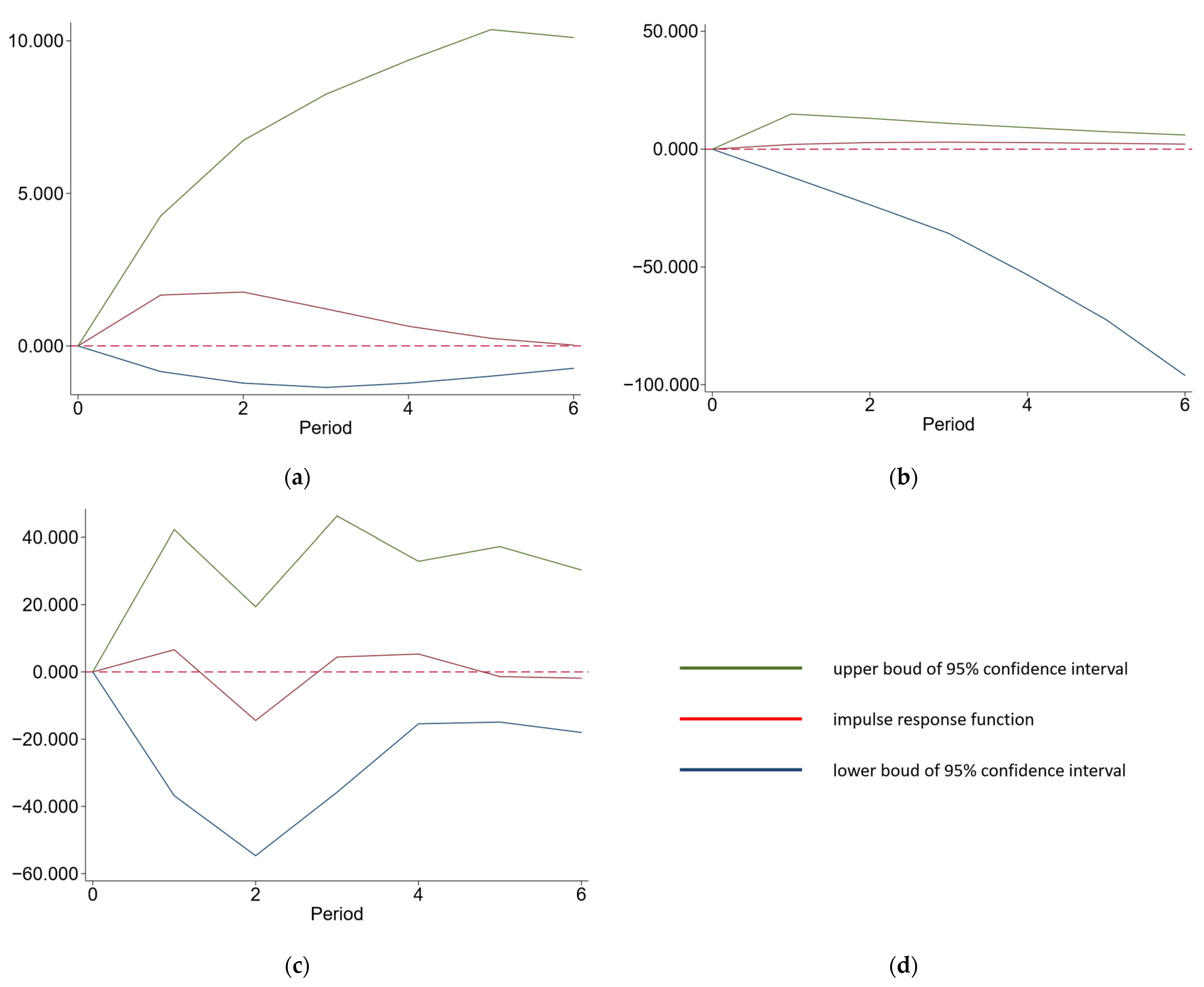
4.3. PVAR

To obtain reliable and meaningful results, the PVAR model requires further consideration of stationarity, cointegration, model order selection, parameter estimation, and impulse response analysis.

Table 7. Stationarity test.

Variable	IPS		Hadri LM		Stationary?
	Statistic	p-Value	Statistic	p-Value
$D{C}_{x_1}$	−0.5465	0.2924	6.3764	0.0000	No
$D{C}_{x_2}$	1.9141	0.9722	3.8648	0.0001	No
$D{C}_{x_3}$	3.9890	1.0000	3.6910	0.0001	No
$D{C}_{x_4}$	−0.9035	0.1831	3.6189	0.0001	No
PG	1.2782	0.8994	7.4962	0.0000	No
$∆D{C}_{x_1}$	−3.7011	0.0001	−0.0754	0.5300	Yes
$∆D{C}_{x_2}$	−0.8035	0.2108	1.3990	0.0809	No
$∆D{C}_{x_3}$	−1.9946	0.0230	1.0105	0.1561	Yes
$∆D{C}_{x_4}$	−2.2975	0.0108	1.0667	0.1430	Yes
$∆$PG	−1.5575	0.0597	0.5273	0.2990	Yes

shows the results of the stationarity test. As shown in this table, we conducted the stationarity test using two methods, the Im-Pesaran-Shin (IPS) test and the Hadri LM test. The utilization of both tests is aimed at validating the outcome’s robustness. In the IPS test, the null hypothesis is that panels have a unit root, which are nonstationary. Whereas, in the Hadri LM test, the null hypothesis is that all the panels are stationary. As for $D{C}_{x_1}$, the p-value of the IPS test is more than 10%. This means that the null hypothesis could not be rejected, indicating that the panel data $D{C}_{x_1}$ might be nonstationary. Meanwhile, the p-value of the Hadri LM test is less than 5%. THis means that the null hypothesis could be rejected, also indicating that the panel data $D{C}_{x_1}$ are nonstationary. By applying the same approach, we can conclude that $D{C}_{x_2}, D{C}_{x_3}, D{C}_{x_4}$ and PG are also nonstationary. When it comes to $∆D{C}_{{\mathrm{x}}_1}$, the first-order difference of $D{C}_{x_1}$, the p-value of the IPS test is less than 5% and the p-value of the Hadri LM test is more than 10%. It can be rejected that $∆D{C}_{{\mathrm{x}}_1}$ is nonstationary; thus, $∆D{C}_{{\mathrm{x}}_1}$ is stationary. By applying the same approach, we can conclude that $∆D{C}_{{\mathrm{x}}_3}$ and $∆D{C}_{{\mathrm{x}}_4}$ are also nonstationary. For $∆D{C}_{x_2}$, the p-value of the IPS test is greater than 10% and the p-value of the Hadri LM test is less than 10%. It cannot reject that $∆D{C}_{x_2}$ is nonstationary; thus, $∆D{C}_{x_2}$ is regarded as nonstationary. When it comes to $∆PG$, the p-value of the IPS test is less than 10% and the p-value of the Hadri LM test is greater than 10%. It can be accepted that $∆PG$ is stationary.

If there are non-stationary variables, it is essential to perform cointegration tests to ascertain the existence of a long-term relationship among them [40]. The presence of cointegration guarantees that the model is not spurious and helps us to prevent making inaccurate conclusions. The PVAR models we intend to build in this paper consist of four two-variable models (see Equation (9)). For a two-variable model, the variables must be integrated in the same order, which is a prerequisite for conducting cointegration tests. It is discovered that $D{C}_{x_1}, D{C}_{x_3}, D{C}_{x_4}$ and PG are all integrated in the same order, but $D{C}_{x_2}$ is not. Thus only $D{C}_{x_1}, D{C}_{x_3}, D{C}_{x_4}$ and PG can be used to conduct further cointegration tests.

Table 8. Pedroni cointegration test.

Model	Variables	MPP		PP		ADF		Cointegrated?
		Statistic	p-Value	Statistic	p-Value	Statistic	p-Value
Model A	$D{C}_{x_1}$~PG	4.5384	0.0000	−12.8980	0.0000	−13.1437	0.0000	Yes
Model B	$D{C}_{x_3}$~PG	4.3562	0.0000	−3.5046	0.0002	−6.5566	0.0000	Yes
Model C	$D{C}_{x_4}$~PG	4.8180	0.0000	−5.7338	0.0000	−5.6927	0.0000	Yes

presents the results of the Pedroni cointegration test. As shown in this table, the p-values in the Modified Phillips–Perron (MPP) test, the Phillips–Perron (PP) test and the Augmented Dickey–Fuller (ADF) test are all less than 5%. The null hypothesis of no cointegration could be rejected. This provides strong evidence that $D{C}_{x_1}$, $D{C}_{x_3}$ and $D{C}_{x_4}$ are cointegrated with PG, respectively, implying that they individually have long-run relationships with PG.

The information criteria method is a commonly used method to determine the lag order of a PVAR model. This method involves selecting the lag order that minimizes a specific information criterion, such as the Akaike information criterion (AIC), Bayesian information criterion (BIC) or Hannan–Quinn information criterion (HQIC) [40]. We estimate PVAR models with different lag orders and compute the AIC, BIC and HQIC values for each model. The results are reported in

Table 9. Lag order selection.

Model	Variables	Lag	AIC	BIC	HQIC
Model A	$D{C}_{x_1}$~PG	1	8.035	9.1703 *	8.4953
		2	7.8960 *	9.2608	8.4505 *
		3	8.1849	9.8574	8.86407
		4	9.2733	11.3843	10.1246
Model B	$D{C}_{x_3}$~PG	1	12.4656	13.6008 *	12.9259 *
		2	12.3905 *	13.7553	12.9449
		3	12.6664	14.3389	13.3457
		4	13.6119	15.7229	14.4632
Model C	$D{C}_{x_4}$~PG	1	14.4839	15.6192	14.9442
		2	16.4120	17.7768	16.9664
		3	14.2679	15.9404	14.9471
		4	13.0424 *	15.1534 *	13.8937 *

Notes: * denotes the minimum value.

.

As shown in Table 9, the best lag order is 2 for Model A. Similarly, the best lag order is 1 for Model B and 4 for Model C. Thus, we can construct the PVAR models in the following way:

$$\left[\begin{array}{c}D{C}_{x_2}^{\left(i,t\right)}\\ P{G}^{\left(i,t\right)}\end{array}\right]=A^{\left(0\right)}+A^{\left(1\right)}\left[\begin{array}{c}D{C}_{x_1}^{\left(i,t-1\right)}\\ P{G}^{\left(i,t-1\right)}\end{array}\right]+A^{\left(2\right)}\left[\begin{array}{c}D{C}_{x_1}^{\left(i,t-2\right)}\\ P{G}^{\left(i,t-2\right)}\end{array}\right]+\left[\begin{array}{c}{\epsilon }_1\\ {\epsilon }_2\end{array}\right]$$

(11)

$$\left[\begin{array}{c}D{C}_{x_3}^{\left(i,t\right)}\\ P{G}^{\left(i,t\right)}\end{array}\right]=B^{\left(0\right)}+B^{\left(1\right)}\left[\begin{array}{c}D{C}_{x_1}^{\left(i,t-1\right)}\\ P{G}^{\left(i,t-1\right)}\end{array}\right]+\left[\begin{array}{c}{\epsilon }_1\\ {\epsilon }_2\end{array}\right]$$

(12)

$$\left[\begin{array}{c}D{C}_{x_4}^{\left(i,t\right)}\\ P{G}^{\left(i,t\right)}\end{array}\right]=C^{\left(0\right)}+C^{\left(1\right)}\left[\begin{array}{c}D{C}_{x_1}^{\left(i,t-1\right)}\\ P{G}^{\left(i,t-1\right)}\end{array}\right]+C^{\left(2\right)}\left[\begin{array}{c}D{C}_{x_1}^{\left(i,t-2\right)}\\ P{G}^{\left(i,t-2\right)}\end{array}\right]+C^{\left(3\right)}\left[\begin{array}{c}D{C}_{x_1}^{\left(i,t-3\right)}\\ P{G}^{\left(i,t-3\right)}\end{array}\right]+C^{\left(4\right)}\left[\begin{array}{c}D{C}_{x_1}^{\left(i,t-4\right)}\\ P{G}^{\left(i,t-4\right)}\end{array}\right]+\left[\begin{array}{c}{\epsilon }_1\\ {\epsilon }_2\end{array}\right]$$

(13)

In this paper, the generalized method of moment (GMM) method is used to estimate the PVAR models.

Table 10. Estimation results.

Variable	$\mathbf{D}{\mathbf{C}}_{{\mathbf{x}}_1}$	$\mathbf{D}{\mathbf{C}}_{{\mathbf{x}}_3}$	$\mathbf{D}{\mathbf{C}}_{{\mathbf{x}}_4}$
$D{C}_{x_1}$ (−1)	0.9855 (4.25)	-	-
$D{C}_{x_1}$ (−2)	−0.1840 (−1.89)	-	-
$D{C}_{x_3}$ (−1)	-	0.7239 (1.75)	-
$D{C}_{x_4}$ (−1)	-	-	0.7068 (4.16)
$D{C}_{x_4}$ (−2)	-	-	−0.1373 (−1.08)
$D{C}_{x_4}$ (−3)	-	-	0.0869 (0.63)
$D{C}_{x_4}$ (−4)	-	-	−0.0610 (−0.75)
PG (−1)	10.1423 (1.04)	9.3295 (0.25)	41.4307 (0.29)
PG (−2)	−8.4300 (−1.50)	-	−145.0264 (−1.98)
PG (−3)	-	-	174.1642 (1.52)
PG (−4)	-	-	−75.5860 (−0.63)

Notes: z-values in parentheses.

reports the estimation results. Unlike traditional structural models, the PVAR model is essentially a reduced form model which does not require precise theoretical framework. This implies that the coefficients may not have explicit economic meanings. Therefore, analysis of the regression results should not focus on individual coefficients, but on the dynamic interactions among variables. This helps in understanding how change in per capita GRP leads to dynamic impacts on variables. Thus, to gain further insights, it is crucial to employ techniques like impulse response analysis.

Figure 2 shows the impulse response function (IRF). The IRF depicts the reaction of each driving effect when there is an impulse in per capita GRP (PG). $D{C}_{x_1}, D{C}_{x_3}, D{C}_{x_4}$ and PG are all integrated in the same order, but $D{C}_{x_2}$ is not. Thus, only $D{C}_{x_1}, D{C}_{x_3}, D{C}_{x_4}$ and PG can be used to conduct impulse response function analysis.

As shown in Figure 2, the energy structure effect ($D{C}_{x_1}$) demonstrates a consistently positive response to economic growth, indicating that when economic growth is subjected to a positive impulse, the energy structure effect in the tourism transport sector tends to increase. This effect reached its peak during the second period, suggesting a strong correlation between economic expansion and carbon emissions during this phase. However, it is noteworthy that this effect gradually declines after reaching its peak. This decline could be attributed to the implementation of more efficient technologies or a shift towards greener practices within the tourism industry as the economic growth continues [9].

The expenditure effect ($D{C}_{x_3}$) also shows a consistent positive response to economic growth. This suggests that increased spending in the tourism sector, likely driven by higher disposable incomes and economic prosperity, contributes to an increase in CO₂ emissions. The variable response of the scale effect suggests that while economic growth can lead to an increase in tourist numbers, the resultant impact on CO₂ emissions can be moderated by implementing sustainable tourism and transportation policies [26,28].

Unlike the energy structure, expenditure and scale effects, which exhibit varying degrees of responsiveness to economic growth, the energy intensity effect ($D{C}_{x_2}$), does not demonstrate a statistically significant long-term relationship with regional economic development. This divergence is noteworthy because it suggests that changes in the energy efficiency of tourism-related transport do not necessarily move in tandem with the regional economic growth.

These findings are significant because they challenge the assumption that economic growth inevitably leads to increased energy consumption and, by extension, increased carbon emissions in the tourism sector. It opens avenues for further research into the factors that drive energy efficiency in tourism-related transport and how these can be leveraged to decouple economic development from environmental impacts. For policymakers, it highlights the potential for targeted interventions to improve energy efficiency without hindering economic growth and provides a pathway towards sustainable development in the tourism industry.

5. Conclusions and Policy Implications

Carbon emissions in tourism are essential for climate change. Existing research only studies the relationship between economic growth and tourism carbon emissions. But we have conducted a more in-depth study of the relationship between economic growth and the driving effects behind tourism carbon emissions. This can more deeply reveal the mechanism of how economic growth influences tourism carbon emissions. This is one of the most important contributions of our work. In addition, the driving effects behind tourism carbon emissions are obtained using the LMDI method. In order to reveal the mechanism of how economic growth influences tourism transport-related CO₂ emissions, this paper has adopted a method using LMDI and PVAR models. An empirical study was conducted in China from 2010 to 2018. Firstly, this paper decomposed the transport-related tourism CO₂ emissions into four driving effects using the LMDI method. Secondly, in response to the deficiency that few studies have examined in the dynamic interactions between the transport-related tourism CO₂ emissions and per capita GRP, this paper established PVAR models based on each driving effect and per capita GRP. This is the major contribution of our work.

This study found that there was a reduction of 939.9393 × 10⁴ tons of CO₂ emissions correlated with the energy structure factor between 2010 and 2018. Meanwhile, the tourism transport CO₂ emissions contributed by the energy intensity factor decreased by 8392.0915 × 10⁴ tons. The adoption of cleaner and more efficient energy has contributed to this trend, mitigating CO₂ emissions by a substantial margin. However, the growth in tourism expenditure and scale has increased CO₂ emissions, underscoring the complex interplay between economic development and environmental sustainability in the tourism sector.

These findings underscore the importance of strategic policies to promote sustainable energy use and efficiency in the tourism transport sector. It acknowledges the adverse impacts of tourism growth on environmental sustainability, particularly through expenditure and scale effects. However, the significant reduction in CO₂ emissions attributed to improved energy structure and efficiency underlines the critical role of promoting green infrastructure, encouraging energy-efficient transport and incentivizing carbon footprint reduction efforts. These strategies are pivotal in reversing the upward trend in carbon emissions and ensuring a sustainable trajectory for the tourism industry.

This study also found a complex interplay between economic growth and CO₂ emissions within the tourism transport sector. Economic growth promotes an increase in CO₂ emissions through the energy structure, expenditure and scale effects, but the lack of a significant cointegration in the energy intensity effect suggests an opportunity to decouple economic development from environmental degradation. This indicates that technological advances and shifts towards sustainable practices can mitigate environmental impacts without compromising economic growth, challenging the assumption that economic prosperity inevitably leads to increased emissions.

These findings also advocate for strategic policy measures to foster green and efficient energy use in the tourism transport sector. Admittedly, the negative impacts of tourism growth on environmental sustainability are recognized, in particular the expenditure effect and scale effect. However, this reduction in CO₂ emissions through improved energy structure and efficiency is important and highlights the important role of promoting advances in green infrastructure and energy-efficient transport and incentivizing carbon footprint reduction efforts. Such strategies would play a critical role in reversing the upward trajectory of emissions and putting the tourism industry on a new and sustainable downward trajectory.

While this paper provides a comprehensive analysis of the driving effects behind tourism transport CO₂ emissions and economic growth, a potential issue is the limited generalizability of the findings. This study also has certain limitations that should be taken into account.

• The data used in this study came from China. More studies should be conducted using the same methodology to ensure the generalizability of the results. It would increase the work’s contribution to the larger subject of sustainable tourism if it addressed potential contextual differences in other countries.
• This study focused on CO₂ emissions from transport in the tourism sector and did not include CO₂ emissions from other tourism activities, such as accommodation. To properly mitigate carbon footprint, a thorough assessment of all CO₂ emissions from tourism is necessary. Further research should fully integrate these aspects.
• It is crucial to acknowledge that external factors such as policy changes or global economic shifts may have an impact on the observed dynamics.

Therefore, further studies emerging from this manuscript should consider the following avenues. First, similar analyses should be conducted in other countries to determine whether the findings presented here are globally representative or unique to China’s pre-pandemic context. Second, the scope of the investigation should extend beyond the transportation segment of tourism to include the accommodation and entertainment industries, both of which play critical roles in the tourism sector and contribute to its environmental footprint. Finally, the study’s finding of a significant reduction in CO₂ emissions due to improved energy structures within the tourism transportation industry requires further investigation. Future research should incorporate micro-level data to pinpoint which sustainable practices effectively suppress CO₂ emissions. Identifying these practices can suggest solid strategies for promoting energy efficiency not just in tourism transport but across the entire tourism sector, offering insights into sustainable development practices and guiding future efforts to minimize environmental impacts.

References

1. Peeters, P.; Cakmak, E.; Guiver, J. Current Issues in Tourism: Mitigating Climate Change in Sustainable Tourism Research. Tour. Manag. 2024, 100, 104820. [Google Scholar] [CrossRef]
2. Jiaqi, Y.; Yang, S.; Ziqi, Y.; Tingting, L.; Teo, B.S.X. The Spillover of Tourism Development on CO2 Emissions: A Spatial Econometric Analysis. Environ. Sci. Pollut. Res. 2022, 29, 26759–26774. [Google Scholar] [CrossRef]
3. Lenzen, M.; Sun, Y.-Y.; Faturay, F.; Ting, Y.-P.; Geschke, A.; Malik, A. The Carbon Footprint of Global Tourism. Nat. Clim. Chang. 2018, 8, 522–528. [Google Scholar] [CrossRef]
4. Gössling, S.; Peeters, P.; Ceron, J.-P.; Dubois, G.; Patterson, T.; Richardson, R.B. The Eco-Efficiency of Tourism. Ecol. Econ. 2005, 54, 417–434. [Google Scholar] [CrossRef]
5. Chen, S.; Tan, Z.; Chen, Y.; Han, J. Research Hotspots, Future Trends and Influencing Factors of Tourism Carbon Footprint: A Bibliometric Analysis. J. Travel Tour. Mark. 2023, 40, 131–150. [Google Scholar] [CrossRef]
6. Rico, A.; Martinez-Blanco, J.; Montlleo, M.; Rodriguez, G.; Tavares, N.; Arias, A.; Oliver-Sola, J. Carbon Footprint of Tourism in Barcelona. Tour. Manag. 2019, 70, 491–504. [Google Scholar] [CrossRef]
7. World Tourism Organization. Climate Change and Tourism: Responding to Global Challenges; World Tourism Organization: Madrid, Spain, 2008; ISBN 978-92-844-1234-1. [Google Scholar]
8. Gunter, U.; Wöber, K. Estimating Transportation-Related CO2 Emissions of European City Tourism. J. Sustain. Tour. 2022, 30, 145–168. [Google Scholar] [CrossRef]
9. Yang, G.; Jia, L. Estimation of Carbon Emissions from Tourism Transport and Analysis of Its Influencing Factors in Dunhuang. Sustainability 2022, 14, 14323. [Google Scholar] [CrossRef]
10. Yang, S.; Duan, Z.; Jiang, X. Spatial Dynamics and Influencing Factors of Carbon Rebound Effect in Tourism Transport: Evidence from the Yangtze-River Delta Urban Agglomeration. J. Environ. Manag. 2023, 344, 118431. [Google Scholar] [CrossRef]
11. Sheng, M.S.; Sharp, B.; Yi, M.; Wen, L.; Suomalainen, K. A Cointegration Analysis of New Zealand’s Economic Development, Fossil Fuel Usage and Transport Emissions. Case Stud. Transp. Policy 2022, 10, 2497–2505. [Google Scholar] [CrossRef]
12. Dai, J.; Alvarado, R.; Ali, S.; Ahmed, Z.; Meo, M.S. Transport Infrastructure, Economic Growth, and Transport CO2 Emissions Nexus: Does Green Energy Consumption in the Transport Sector Matter? Environ. Sci. Pollut. Res. 2023, 30, 40094–40106. [Google Scholar] [CrossRef] [PubMed]
13. Go, Y.-H.; Lau, L.-S.; Liew, F.-M.; Senadjki, A. A Transport Environmental Kuznets Curve Analysis for Malaysia: Exploring the Role of Corruption. Environ. Sci. Pollut. Res. 2021, 28, 3421–3433. [Google Scholar] [CrossRef] [PubMed]
14. Kharbach, M.; Chfadi, T. CO2 Emissions in Moroccan Road Transport Sector: Divisia, Cointegration, and EKC Analyses. Sustain. Cities Soc. 2017, 35, 396–401. [Google Scholar] [CrossRef]
15. Luo, F.; Moyle, B.D.; Moyle, C.J.; Zhong, Y.; Shi, S. Drivers of Carbon Emissions in China’s Tourism Industry. J. Sustain. Tour. 2020, 28, 747–770. [Google Scholar] [CrossRef]
16. De Boer, P.; Rodrigues, J.F.D. Decomposition Analysis: When to Use Which Method? Econ. Syst. Res. 2020, 32, 1–28. [Google Scholar] [CrossRef]
17. Luo, X.; Liu, C.; Zhao, H. Driving Factors and Emission Reduction Scenarios Analysis of CO2 Emissions in Guangdong-Hong Kong-Macao Greater Bay Area and Surrounding Cities Based on LMDI and System Dynamics. Sci. Total Environ. 2023, 870, 161966. [Google Scholar] [CrossRef] [PubMed]
18. Tang, M.; Ge, S. Accounting for Carbon Emissions Associated with Tourism-Related Consumption. Tour. Econ. 2018, 24, 510–525. [Google Scholar] [CrossRef]
19. Safaa, L.; Atalay, A.; Makutėnienė, D.; Perkumienė, D.; Bouazzaoui, I.E. Assessment of Carbon Footprint Negative Effects for Nature in International Traveling. Sustainability 2023, 15, 12510. [Google Scholar] [CrossRef]
20. Li, X.-Y.; Chen, T.; Chen, B. Research on the Influencing Factors and Decoupling State of Carbon Emissions in China’s Transportation Industry. Sustainability 2023, 15, 11871. [Google Scholar] [CrossRef]
21. Chen, Q.; Mao, Y.; Morrison, A.M. Impacts of Environmental Regulations on Tourism Carbon Emissions. Int. J. Environ. Res. Public Health 2021, 18, 12850. [Google Scholar] [CrossRef]
22. Pablo-Romero, M.d.P.; Sanchez-Braza, A.; Sanchez-Rivas, J. Tourism and Electricity Consumption in 9 European Countries: A Decomposition Analysis Approach. Curr. Issues Tour. 2021, 24, 82–97. [Google Scholar] [CrossRef]
23. Chen, L.; Hang, Y.; Li, Q. Spatial-Temporal Characteristics and Influencing Factors of Carbon Emissions from Land Use and Land Cover in Black Soil Region of Northeast China Based on LMDI Simulation. Sustainability 2023, 15, 9334. [Google Scholar] [CrossRef]
24. Gołaś, Z. Changes in Energy-Related Carbon Dioxide Emissions of the Agricultural Sector in Poland from 2000 to 2019. Energies 2022, 15, 4264. [Google Scholar] [CrossRef]
25. Zhang, J.; Zhang, Y. Tourism, Economic Growth, Energy Consumption, and CO2 Emissions in China. Tour. Econ. 2021, 27, 1060–1080. [Google Scholar] [CrossRef]
26. Zha, J.; Dai, J.; Ma, S.; Chen, Y.; Wang, X. How to Decouple Tourism Growth from Carbon Emissions? A Case Study of Chengdu, China. Tour. Manag. Perspect. 2021, 39, 100849. [Google Scholar] [CrossRef]
27. Parker, S. A Decoupling Analysis of Transport CO2 Emissions from Economic Growth: Evidence from Vietnam. Int. J. Sustain. Transp. 2022, 16, 928–941. [Google Scholar] [CrossRef]
28. Tang, Q.; Wang, Q.; Zhou, T. Driving Forces of Tourism Carbon Decoupling: A Case Study of the Yangtze River Economic Belt, China. Sustainability 2022, 14, 8674. [Google Scholar] [CrossRef]
29. Issayeva, G.; Dyussembekova, Z.; Aidarova, A.B.; Makhatova, A.B.; Lukhmanova, G.; Absemetova, D.; Bolganbayev, A. The Relationship between Renewable Energy Consumption, CO2 Emissions, Economic Growth, and Industrial Production Index: The Case of Kazakhstan. Int. J. Energy Econ. Policy 2023, 13, 1–7. [Google Scholar] [CrossRef]
30. Triatmanto, B.; Bawono, S.; Wahyuni, N. The Contribution and Influence of Total External Debt, FDI, and HCI on Economic Growth in Indonesia, Thailand, Vietnam, and Philippines. Res. Glob. 2023, 7, 100163. [Google Scholar] [CrossRef]
31. Afjal, M. The Tapestry of Green Economics: Mapping the Nexus of CO2 Emissions, Economic Growth, and Renewable Energy. Int. J. Sustain. Energy 2023, 42, 1364–1390. [Google Scholar] [CrossRef]
32. Li, W.; Hao, N.; Lu, C. A PVAR Dynamic Correlation Appraisal of China’s Carbon Emissions in Conjunction with Economic Growth and Clean Energy Use. Renew. Energy 2023, 219, 119484. [Google Scholar] [CrossRef]
33. Jahanger, A.; Hossain, M.R.; Awan, A.; Sunday Adebayo, T.; Zubair Chishti, M. Linking Tourist’s Footprint and Environmental Tragedy through Transportation, Globalization and Energy Choice in BIMSTEC Region: Directions for a Sustainable Solution Using Novel GMM-PVAR Approach. J. Environ. Manag. 2023, 345, 118551. [Google Scholar] [CrossRef]
34. Zhang, Y.; Hong, W.; Huang, Q.; Liu, C. Heterogeneous Effects of Urbanization, Economic Growth, and Energy Consumption on Carbon Emissions in China: Evidence from a PVAR Model. Air Qual. Atmos. Health 2023, 16, 2471–2498. [Google Scholar] [CrossRef]
35. Jiang, G.; Zhu, A.; Li, J. Measurement and Impactors of Tourism Carbon Dioxide Emission Efficiency in China. J. Environ. Public Health 2022, 2022, 9161845. [Google Scholar] [CrossRef] [PubMed]
36. Su, J. Impact of Tourism Resource Development Based on Low-Carbon Mode: A Case Study of Guizhou Ethnic Areas. Ecol. Process. 2019, 8, 21. [Google Scholar] [CrossRef]
37. Pan, Y.; Weng, G.; Li, C.; Li, J. Coupling Coordination and Influencing Factors among Tourism Carbon Emission, Tourism Economic and Tourism Innovation. Int. J. Environ. Res. Public Health 2021, 18, 1601. [Google Scholar] [CrossRef]
38. Guo, S.; Liu, G.; Liu, S. Driving Factors of NOX Emission Reduction in China’s Power Industry: Based on LMDI Decomposition Model. Environ. Sci. Pollut. Res. 2023, 30, 51042–51060. [Google Scholar] [CrossRef]
39. Peng, H.; Zhang, J.; Lu, L.; Tang, G.; Yan, B.; Xiao, X.; Han, Y. Eco-Efficiency and Its Determinants at a Tourism Destination: A Case Study of Huangshan National Park, China. Tour. Manag. 2017, 60, 201–211. [Google Scholar] [CrossRef]
40. Dai, S.; Wang, Y.; Zhang, W. The Impact Relationships between Scientific and Technological Innovation, Industrial Structure Advancement and Carbon Footprints in China Based on the PVAR Model. Int. J. Environ. Res. Public Health 2022, 19, 9513. [Google Scholar] [CrossRef]
41. Nishiyama, H.; Gintani, Y.; Tsuboi, M. The Impact of Trade on Growth and Welfare with Heterogeneous Firms and Rent-Sharing. Int. Rev. Econ. Financ. 2024, 89, 731–742. [Google Scholar] [CrossRef]
42. Niu, J.; Chen, X.; Sun, S. China’s Coal Ban Policy: Clearing Skies, Challenging Growth. J. Environ. Manag. 2024, 349, 119420. [Google Scholar] [CrossRef] [PubMed]
Figure 1. The study area. (source National Geomatics Center of China).
Sustainability 16 03135 g001
Figure 2. The impulse response functions. (a) Response of  D C x 1  to PG; (b) response of  D C x 3  to PG; (c) response of  D C x 4  to PG; (d) legend.
Sustainability 16 03135 g002