Abstract
In South Africa, the agricultural sector is a crucial pillar of the economy, with the livestock and grain industries playing significant roles in ensuring food security, fostering economic growth, and providing employment opportunities, particularly in rural areas. This research addresses the relatively unexplored relationship between the livestock and grain industries in South Africa. This study employs a comprehensive approach using a VAR/VECM framework alongside VECM Granger causality tests, Toda Yamamoto causality tests, impulse response functions, and variance decomposition analysis. The main findings of this study demonstrate a long-run relationship among the study variables, with consistently low error correction terms indicating slow short-term adjustments. Significant long-run relationships were observed between grain feed prices and livestock prices, where yellow maize and soybean prices affect live weaner prices, while beef carcass prices influence yellow maize prices. Overall, the results highlight the pivotal role that yellow maize plays as a link between the South African livestock and grain markets. The study concluded that policy formulation for the South African agricultural sector must consider the interconnected nature of the grain and livestock markets to achieve sustainable and effective outcomes.
1. Introduction
The South African agricultural sector, while modest in its overall contribution to the national economy, plays a pivotal role in ensuring accessible food and fostering economic growth, and serves as a significant employment source, particularly in rural areas [1]. The sector’s diversity, encompassing field crops, horticulture, and animal production, significantly shapes the nation’s food security landscape. According to DALRRD [1], the livestock industry is a dominant contributor, constituting 41.7% of South Africa’s total agricultural gross value, followed closely by field crops and horticulture, which contribute 31.5% and 26.8%, respectively.
The interconnections between livestock and field crops in South Africa are notable, with ties established through supply and demand dynamics in feed-related channels. Field crops like maize and soybeans are essential feed sources for the livestock industry. According to AFMA [2], livestock feeds in South Africa mainly consist of maize (51.22%) and various oilcake (20.63%), with soybean oilcake contributing around 71% to the total oilcake percentage. Furthermore, NAMC [3] indicated that approximately 70% of South Africa’s yellow maize demand during the 2022–2023 marketing year was attributed to the livestock industry. In the same marketing year, 9% of the total demand for soybeans in South Africa was attributed to full-fat soybeans, while 77% was attributed to soybean oilcake, both essential components in livestock feed. The statistics presented strongly suggest a significant interdependence between the grain and livestock industries in South Africa, indicating a noteworthy relationship that is still relatively unexplored in the literature. According to Gardebroek et al. [4], the close interconnection among agricultural commodities stems from their roles as substitutes in demand, common input costs, competition for limited natural resources, and access to shared market information. Understanding the livestock and grain industry relationship is crucial for ensuring food security, supporting economic growth, and promoting sustainable agricultural and food systems.
One crucial dimension in considering the various aspects of food security involves examining the inter-price relations within commodity markets [5]. Surging price spillovers have the potential to lead to high inflation rates, large trade deficits, and unfavorable macroeconomic environments, especially in developing economies [6]. A thorough understanding of commodity price spillovers is essential for navigating global markets [7], predicting trends [8], managing financial risks [9,10], and fostering sustainable agricultural practices [11] to enhance economic resilience and food security overall. The importance of investigating price and volatility transmission dynamics across diverse commodity markets is evident based on the attention it has consistently received in the literature over time.
However recent black swan events such as the COVID-19 pandemic and the Russia–Ukraine invasion have renewed interest in commodity price volatility and dynamic spillovers [10,11,12,13,14,15,16,17]. This renewed interest underscores the importance of further investigating price and volatility transmission dynamics across diverse commodity markets. Notably, studies in South Africa have examined various aspects of price transmissions over time, encompassing both vertical and horizontal price spillover dynamics within the agricultural sector.
Moreover, complementary to this broader examination, studies have specifically explored vertical price transmissions within South African value chains. For instance, Alemu [18] examined the relationship between producer and retail markets within South Africa’s food market. Similarly, research has investigated vertical transmission within key sectors such as the South African poultry industry [19], providing valuable insights into the interactions between different stages of production and distribution. Additionally, a study conducted by Lombaard [20] explored the South African beef value chain, offering further understanding of the vertical transmission mechanisms within the beef sector. In addition, Mosese [21] specifically examined vertical transmission in the South African potato value chain, while Louw [22] investigated price transmission in wheat-to-bread and maize-to-maize meal value chains.
In contrast, other studies have focused on horizontal price spillovers, exploring how price changes among related products influence one another within the same level of the supply chain. Kirsten [23] examined how international commodity markets impact local prices in South Africa, specifically investigating the dynamic relationships between global maize and wheat prices and their counterparts in South Africa. Abidoye and Labuschagne [24] studied the transmission of world maize prices to South African maize prices. Pierre and Kaminski [25] focused on price transmission in South Africa’s maize markets and those of other African countries. Mokumako and Baliyan [26] investigated the price dynamics between the South African and Botswanan maize markets. Myers [27] studied maize price transmission between South Africa and Zambia. Mphateng [28] assessed the transmission prices between world wheat prices and South African wheat prices. Ramoroka [29] investigated inter-commodity producers’ price transmission between wheat and maize in South Africa. Pierre and Kaminski [25] explored short-run price shock propagation among Sub-Saharan African maize markets, of which South Africa formed a part.
Despite the aforementioned research efforts directed at understanding the various dimensions of price transmissions within South Africa’s agricultural sector, a significant gap in the literature is evident. There remains a significant gap regarding the dynamics of important grain feed prices and their impact on the livestock market in South Africa. Given the interconnected nature of South Africa’s livestock and grain industry and the possible consequences of significant price spillovers, it is essential to develop a comprehensive understanding of the inter-price dynamics of these markets. Failure to understand the relationship between South Africa’s grain and livestock markets hinders effective policymaking, strategic planning by industry stakeholders, and academic advancements within the South African agricultural context. Therefore, considering this gap, the objective of this study is to provide a comprehensive understanding of the interdependence and dynamics between the livestock and grain markets in South Africa. The primary research question guiding our investigation is: What are the dynamics of price transmissions between these two markets, and how can understanding these dynamics contribute to enhancing market efficiency and stability within the South African agricultural context? The findings obtained from our research are anticipated to be valuable for informing decision-making and enhancing understanding of the dynamics within the South African agricultural sector. Specifically, by investigating the dynamics of price transmissions between these key markets, our research not only addresses a critical knowledge gap but also provides valuable insights that directly contribute to improving South Africa’s food security landscape. Understanding price dynamics in these sectors helps identify potential disruptions or vulnerabilities that could affect food availability and affordability, ultimately impacting food security.
2. Materials and Methods
2.1. Data
This study utilized secondary data comprising six distinct time series of weekly prices. The data include weekly spot prices (R/Kg) for live weaners and carcass prices for A2/A3 lamb and beef obtained from the Red Meat Producers Organization (RPO). Additionally, daily spot prices (R/ton) for maize and soybeans were sourced from the Johannesburg Stock Exchange (JSE) and the South African Grain Information Services (SAGIS). In order to ensure that the livestock and grain prices were in the same interval, daily grain prices were aggregated into weekly prices. The datasets cover the period from January 2018 to October 2023.
2.2. Methods
The data collected for this research were analyzed in the STATA version 15 econometric package [30]. To achieve the objectives of this study, a multivariate time series approach was applied to the model to explain the interactions among the variables. Given the time-dependent nature of the data and the need to capture both short-term dynamics and long-run equilibrium relationships, we employed a vector autoregressive (VAR) and vector error correction model (VECM) framework. An overview of the complete methodology is presented in Figure 1.
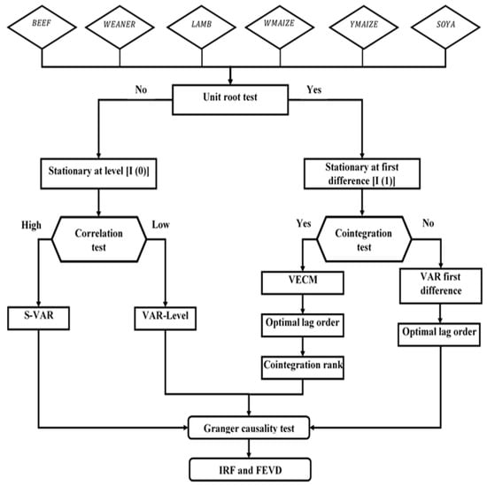
Figure 1.
Comprehensive modelling with VAR and VECM analysis. Note: The figure describes the VECM fitting process for key South African agricultural variables—BEEF (beef carcass price), WEANER (live weaner price), LAMB (lamb carcass price), WMAIZE (white maize price), YMAIZE (yellow maize price), and SOYA (soybean price). Source: adopted and adjusted from Badaoui et al. [31].
2.3. Unit Root Test
This study applied the augmented Dickey–Fuller (ADF) test to assess the stationarity properties of the time series under investigation. Dickey and Fuller [32] proposed the ADF test as an extension of the original standard Dickey and Fuller (DF) test [33]. The standard DF test assumes that the errors in the model are serially uncorrelated. However, in the presence of autocorrelation, the DF test could lead to incorrect conclusions. The ADF test addresses autocorrelation by assuming the series will follow an AR(p) process. The ADF test extends the standard DF test by introducing p-lagged-difference terms of the dependent variable. The ADF test is based on ordinary least squares (OLS) and estimated by Equation (1):
where is the first difference of the variable at time , is the linear deterministic time trend, is the coefficient associated with time trend , is the order of augmentation of the test, is the white noise error term, is the intercept term, and is the coefficients associated with each lagged difference. The null hypothesis implies the presence of a unit root or non-stationarity in the time series ( = 0), while the alternative hypothesis ( < 0) suggests the absence of a unit root. The rejection of the null hypothesis indicates that the series is non-stationary, and vice-versa.
2.4. Cointegration Test
If a unit root is confirmed in the variables, then the next step is to determine whether there is a long-run equilibrium association among the variables. Cointegration is a key concept when dealing with non-stationary time series. If variables are cointegrated, they share a long-term relationship despite exhibiting short-term fluctuations, even if each variable is considered non-stationary. The implementation of the Engle–Granger cointegration test [34] is relatively straightforward. However, it is not well suited for assessing the presence of more than one cointegrating vector. If the data involve multiple cointegrating relationships, relying solely on the Engle–Granger test may yield inaccurate results. Given the limitations of the Engle–Granger cointegration test, particularly its suitability for examining multiple cointegrating vectors, this study employed the Johansen multivariate cointegration test [34,35]. The Johansen cointegration test allows for the identification of multiple cointegrating vectors in a multivariate system. The Johansen cointegration test begins with the estimation of a VAR model. Consider the matrix form of a VAR(p) model in Equation (2):
In Equation (2), accents have been added beneath each matrix component to signify specific elements in the system. This visual notation aids clarity, distinguishing variables, coefficients, and lagged terms. To facilitate a clear understanding of the Johansen cointegration test derivation, Equation (2) can be rewritten in the matrix equation format:
where is an vector of variables that are integrated from order one (denoted as ), t is the time index, is an vector of innovations, is the coefficient matrix associated with the maximum lag order , and is an vector of constant terms. …, are an vector representing the lagged endogenous variables at times , …, . According to the Engle–Granger representation theorem [36], if the variables in Equation (3) are cointegrated, Equation (3) can be rewritten as a VECM in the form of:
where and . Furthermore, ∏ represents the matrix of cointegrating vectors. Johansen’s cointegration test estimates the cointegration rank (∏), indicating the number of cointegrating vectors in the system. The cointegration rank matrix (∏) can be decomposed into ∏ = , where measures the speed at which the variables adjust to their equilibrium (adjustment parameter) and represents the long-run cointegration relationships between variables. Furthermore, the matrices are the coefficients associated with the lagged differences () and represent the short-run adjustment parameters. Johansen’s test employs a maximum likelihood procedure and uses the trace () and maximum eigenvalue () statistics to draw inferences about the existence and quantity of cointegrating vectors within a system, which is expressed as:
where is the number of cointegrated vectors, is the estimated value for the th-order eigenvalue from the ∏ matrix, is the total sample size, and is the total number of variables in the system. The trace test statistic tests the null hypothesis that the rank (∏) = versus the alternative that the rank (∏) > . The trace statistic test is a sequential test that starts with the null hypothesis of = 0 against the alternative hypothesis that the rank is greater than zero. The process is repeated, updating the null hypothesis to higher ranks until it can no longer be rejected. The maximum eigenvalue test, on the other hand, tests the null hypothesis that the rank (∏) = versus the alternative that the rank (∏) =. The maximum eigenvalue test is also a step-by-step procedure, where the null hypothesis starts with = 0 against the alternative that = 1. Similar to the trace statistic, this process is repeated, increasing by one at each step until the null hypothesis cannot be rejected. In both tests, the critical values are compared to the calculated test statistics to make decisions about the presence and number of cointegrating relationships.
2.5. Vector Error Correction Model (VECM)
The results from the Johansen cointegration test provide insights into the cointegration structure of the variables in the system and whether to fit a VAR or VECM model. If cointegration is present, indicating a long-term equilibrium, a VECM is employed since a VECM captures both short-term dynamics and long-term equilibrium equations. If no cointegration is detected, it suggests no stable long-term relationship among variables in the system. In such a case, a VAR model in first differences is a suitable choice since VAR models capture the short-term dynamics and interactions among variables. In the absence of cointegration, the matrix form a VAR() for the study variables can be presented as:
where is the difference operator; , …. are constant values associated with each study variable; indicates the optimal lag length; and , , … are the random error terms. The confirmation of cointegration among a system of variables indicates a long-term relationship among them. In such a case, the VECM is estimated due to its capabilities in estimating the short- and long-run coefficients. Essentially, the VECM can assist in analyzing long-run equilibrium relationships among variables and the short-run deviations from this equilibrium. According to Levendis [37], one key strength of a VECM is that it is convenient to combine the short-term predictive power of VARs with the long-term predictive power of ECMs. The VECM specification for the study variables is structured as follows:
Here, represents the error correction term lagged by one period, and ,, …. are the coefficients of the error term specifying the tendency for the endogenous variables to return to long-run equilibrium. It is crucial for the error correction term () to be negative and significant, as it signifies the presence of a dynamic adjustment mechanism that effectively restores equilibrium following short-term deviations.
2.6. Causality Tests
After determining the cointegration relationship between variables, a Granger causality test was conducted to establish the causal relationships between the study variables. The Granger causality test [38] has been widely applied to assess whether past values of one variable contribute useful information to predicting another variable. According to Johansen [36], if the Granger causality test is conducted on a VAR model in first differences while the considered variables are cointegrated, then the inferences drawn from the causality test might be inaccurate. Therefore, in the presence of cointegration, the Granger causality test is applied to the VECM framework described in the previous section. From Equation (8), long-run causality is indicated by the significance of the one-period lagged error correction term, while the significance of a joint F-test on the sum of the lagged explanatory variables represents the short-run causality.
Toda and Yamamoto [39] recommended against applying the Granger causality test to a VECM model because it might give incorrect results due to biases in preliminary tests, especially related to stationarity and cointegration. In response to these limitations, Toda and Yamamoto [39] proposed a causality test that is robust to the integration and cointegration properties of any or all of the variables in a given system. This study therefore first applied the standard Granger causality test on the VECM and subsequently incorporated the Toda and Yamamoto [39] causality test as a complementary assessment test.
The Toda and Yamamoto [39] procedure entails estimating an augmented VAR model. The augmentation is achieved by extending the VAR model’s lag order by adding extra lag(s). The additional lags to be added are determined by the maximum order of integration () among the variables considered within the system. The augmented lags () are then combined with the optimal lag order () identified for the variables in the VAR system. The Toda and Yamamoto [39] causality test for a bivariate ( ) relationship is presented as follows:
where is the maximum order of integration of the variables in the system. For example, if is integrated of order zero ((0)) and Is integrated of order 2 ((2)), then the maximum order is 2, denoted as = 2. is the optimal lag length of the variables, with and representing the white noise error terms. A modified Wald test is then applied to the first VAR coefficient matrix using the standard chi-square () statistics to test for restrictions on the parameters of the VAR() model, whereas the coefficient matrices for the last lagged vectors in the model are ignored. The null hypothesis assumes no Granger causality, whereas the alternative hypothesis suggests the presence of Granger causality. For Equation (9), the null hypothesis posits that does not Granger cause , expressed as . Conversely, the alternative hypothesis suggests that Granger causes if . Similarly, for Equation (10), the null hypothesis () asserts that does not Granger cause , stated as , whereas the alternative hypothesis () asserts that granger causes if . Specifying the Toda and Yamamoto [39] causality test for our study variables, the augmented VAR model takes the following structure:
In order to assess the causal relationships between the study variables, we imposed a set of restrictions on the augmented VAR model, shown in Equation (11). Table 1 presents the specifications for both the null and alternative hypotheses, outlining the constraints imposed on the matrix coefficients as defined in Equation (11).

Table 1.
Toda and Yamamoto causality test hypotheses for the study variables.
2.7. Impulse Response Function
The Toda causality test only provided the direction of causality for the study period. However, causality tests do not illustrate how each variable responds to a one-unit shock in itself or in another variable in the system. Therefore, impulse response functions were employed to obtain insights into the temporal patterns of responses and the persistence of shocks in the system. Variance decomposition was be employed, as it focuses on quantifying the relative contributions of different variables (including their past values) to the overall variability of each variable in the system. Employing impulse response functions and variance decomposition provides valuable information about the dynamic relationships among the prices of .
3. Results
3.1. Unit Root Test
Table 2 displays the ADF tests’ outcomes on variables in their original levels and first differences. The ADF test aims to assess the stationarity properties of time series data, a crucial step in time series analysis. In applying the ADF test, we included four lags in our model. In Table 2, the ADF test statistics for variables in levels (, , , , , and ) suggest non-stationarity, as their test statistic in absolute values are below the critical values at the 1%, 5%, and 10% levels. Notably, the first differences (∆) of all variables exhibit highly negative ADF test statistics, which are well above the critical values in absolute values, providing strong evidence against the presence of unit roots (all p-values = 0.0000). The results in Table 2 suggest that the first differencing process successfully induced stationarity in the variables, suggesting that all the variables in the study were integrated in the order of one ((1)).
Table 2.
Augmented Dickey–Fuller test results for stationarity.
3.2. VAR Lag Order Selection
In order to identify the most suitable lag order for our analysis, an optimal lag selection was performed using multiple information criteria. The utilized information criteria encompass the log-likelihood (LL), likelihood ratio (LR), degrees of freedom (df), p-value, final prediction error (FPE), Akaike information criterion (AIC), Hannan–Quinn information criterion (HQIC), and Schwarz Bayesian information criterion (SBIC). The outcomes of the lag selection process are summarized in Table 3.
Table 3.
Results of optimal lag selection.
Table 3 shows that lag orders 1, 2, and 5 are marked with asterisks, indicating that these lag orders were optimal based on various information criteria. This study’s identified optimal lag length was 2, based on the HQIC and the AIC. The robustness of the lag selection process was ensured by examining the residuals obtained from fitting a VAR(2) model and testing for autocorrelation using the Lagrange multiplier test. The results of the Lagrange multiplier test in Table 4 further validate the appropriateness of the chosen lag length.
Table 4.
Lagrange multiplier test results for autocorrelation in residuals.
3.3. Cointegration Test
Based on the ADF test results, all the variables were considered integrated in the order of one ((1)). Therefore, the next step was to test whether a long-term relationship existed among the study variables. Based on the results in Table 5 and Table 6, the Johansen cointegration test suggested a long-term relationship among the variables. However, there was a discrepancy between the results of the trace statistic (Table 5) and the maximum eigenvalue (Table 6) regarding the order of the cointegrating rank. The trace statistic suggested an identified rank of 2, indicating the presence of at least two cointegrating vectors.
Table 5.
Results of the Johansen cointegration test (trace).
Table 6.
Results of the Johansen cointegration test (maximum eigenvalue).
On the other hand, the maximum eigenvalue statistic pointed to an identified rank of 1, implying the presence of at least one cointegrating vector. Despite the discrepancy between the trace statistic and maximum eigenvalue discrepancy, this study relied on the trace statistic test. The decision to rely on the trace statistic is supported by the findings of Lüutkepohl et al. [40], who demonstrated that the trace test exhibits superior performance and less distortion in situations with multiple cointegrating relations.
3.4. Vector Error Correction Model (VECM) Estimation
The confirmation of cointegration from the Johansen cointegration test suggests that the variables in the system shared a long-run relationship. Therefore, the VECM was suitable for modelling the relationship among live weaner prices, lamb and beef carcass prices, and prices of white maize, yellow maize, and soybeans. The estimates derived from the VECM served as an initial basis for understanding the causality among the variables, encompassing both short-term and long-term dynamics. The estimates of the VECM are presented in Table 7.
Table 7.
Summary of results of VECM in the short run.
The VECM estimates in Table 7 indicate that the first lagged error correction term () in the beef (), lamb (), weaner (), and white maize () equation was negative and significant at a 1% level. The negative significant term implies that in the equations of beef carcass prices (), lamb carcass prices (), live weaner prices (), and white maize prices (), the system corrected its previous week’s disequilibrium, indicating a gradual correction toward the long-run equilibrium within the weekly time frame of the data. The magnitude of the significant first-lagged error correction term () coefficients varied across equations. In the beef equation (), was −0.02, implying that the system corrected the previous week’s disequilibrium at a speed of 2% per week. Similarly, in the lamb equation (), an adjustment speed of 13% per week was observed, with an coefficient of −0.13. Weaner () demonstrated a correction speed of 7% per week, as indicated by the significant coefficient of −0.07. White maize () showed a significant coefficient of −0.1162, suggesting a rapid adjustment of 11.62% per week. In contrast, the yellow maize equation showed a non-negative and non-statistically significant coefficient. However, was found to be significant at the 1% level, with a coefficient of −0.088, implying a speed of adjustment of 8.8% per week. In contrast, soybean () did not reveal a significant adjustment in either or .
Since the Johansen cointegration test indicated that two cointegrating relationships existed among the study variables, two cointegrating relationships were specified. Table 8 shows that the Johansen identification placed four constraints. In the first cointegrating equation (), the coefficient of live weaner prices () was normalized to one and lamb carcass prices were set equal to zero (dropped). The restrictions were based on the fact that live weaners are often fed with grains such as yellow and white maize and soybeans. The omission of lamb carcass prices aimed to narrow the focus to the relationship between live weaner prices () and grain prices. It is important to note that this normalization scheme was not based on a specific economic theory but rather on a general understanding of the feeding practices for live weaners in South Africa.
Table 8.
Johansen normalized cointegrating coefficients for equations and .
In the second cointegrating equation (), yellow maize () was set to unitary, and white maize () was dropped (set to zero). The restrictions imposed for were guided by AFMA [2] statistics, which indicate that roughly 50% of livestock feeds consist of yellow maize. Additionally, the decision to drop white maize from the second cointegrating equation was based on the higher usage of yellow maize and soybean in livestock feeds than white maize. In the long run, elasticities were exactly identified, and the Johansen normalization restrictions were imposed. The normalized cointegration coefficients are shown in Table 8.
The first normalized cointegration () equation from Table 8 can be mathematically expressed as:
Equation (12) shows that in the long run, live weaner prices () displayed a positive and statistically significant association with beef carcass prices (), soybean prices (), and yellow maize prices (), with coefficients of 0.820, 0.0012, and 0.0106, respectively. This suggests that increased beef carcass, soybean, or yellow maize prices positively impact live weaner prices. Conversely, the coefficient of −0.0163 for white maize prices () indicated a negative and statistically significant effect, signifying that an increase in white maize prices is linked to a decrease in live weaner prices in the long run. The second cointegrating () equation derived from Table 8 is expressed as:
The normalized cointegrating equation for yellow maize revealed that its prices were positively and significantly related to beef carcass prices (), soybean prices (), and live weaner prices (), denoted by the coefficients 141.0689, 0.10216, and −94.22544, respectively. Therefore, increases in beef carcass, soybean, and live weaner prices are associated with corresponding positive movements in yellow maize prices. Additionally, lamb carcass prices () had a positive but non-significant impact on yellow maize prices in the long run.
3.5. Post-Estimation Stability Checks
In this study, we conducted a comprehensive evaluation of the fitted VECM model by examining the serial correlation (LM test), normality test (Jarque–Bera test), and model stability (eigenvalue stability) to ensure the validity of the statistical inferences. The residuals were normally distributed, based on the Jarque–Bera test result in Table 9.
Table 9.
Jarque–Bera test result.
The Lagrange multiplier test in Table 10 shows that at the 5% level, we cannot reject the null hypothesis that no autocorrelation existed in the residuals for any of the orders tested. Thus, the findings suggest that there is no evidence of model misspecification.
Table 10.
Lagrange multiplier test result.
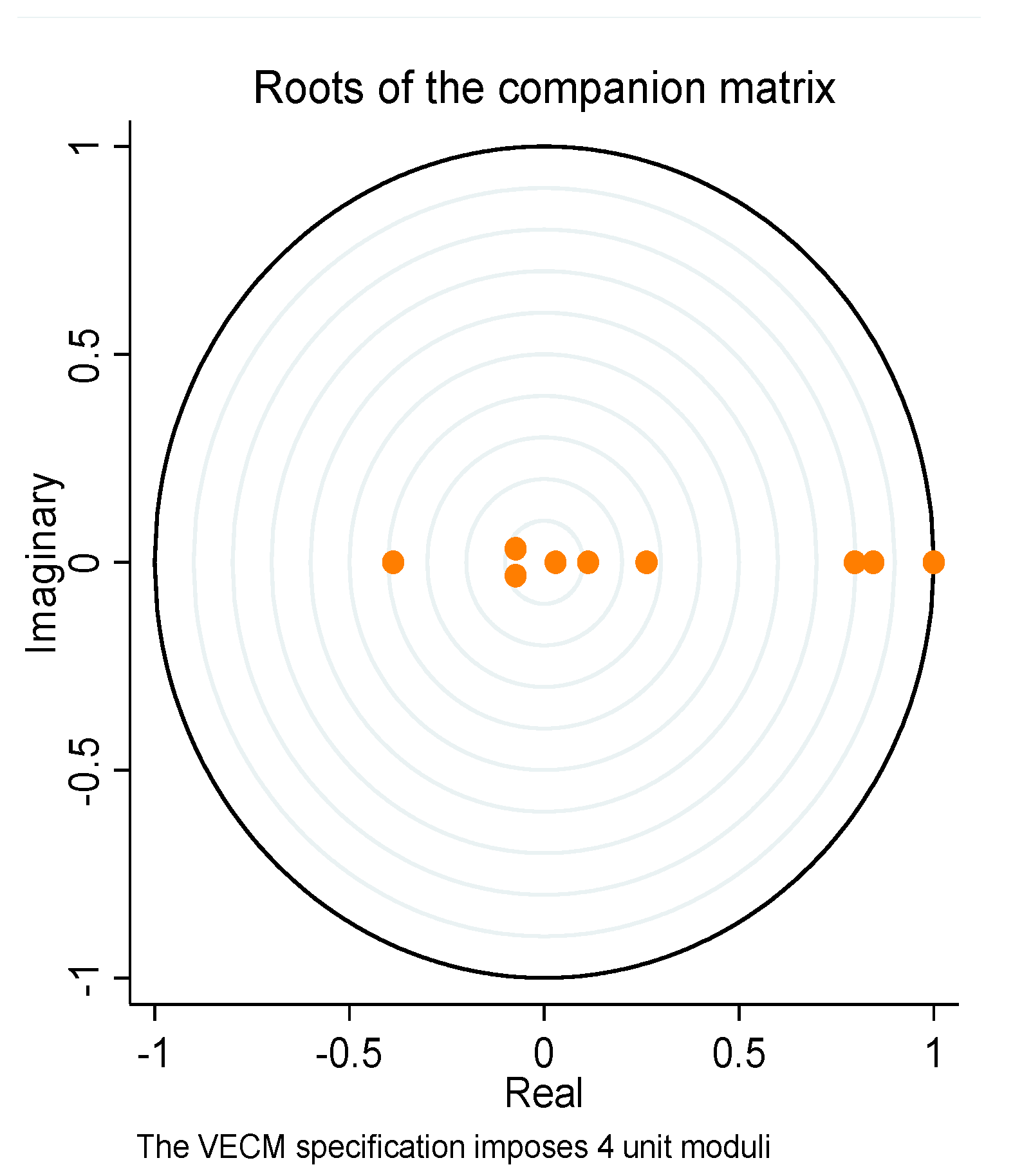
To verify the stability of the specified VECM, we employed the inverse root of AR polynomials. Figure 2 shows that the modulus of each eigenvalue was strictly less than one, and therefore, the estimated VECM was stable.
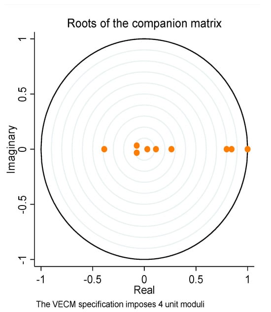
Figure 2.
Stability check for VECM (inverse root of AR polynomials). Source: authors’ compilation.
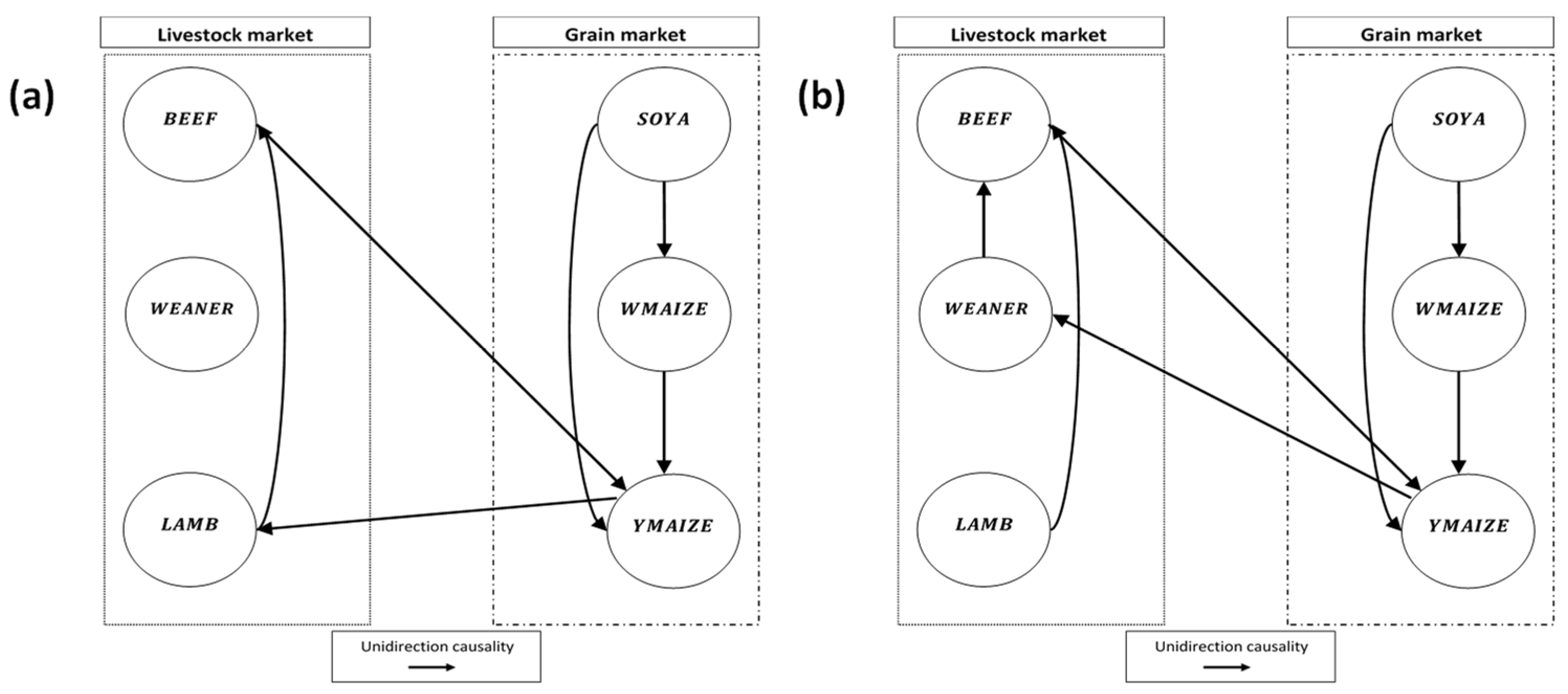
The Granger causality test was utilized to determine causal relationships between variables, evaluating whether past values of one variable contained significant information for predicting the current values of another. Table 11 displays the VECM Granger causality results, highlighting several significant relationships among the variables. Notably, lamb carcass prices predictively influenced beef carcass prices. Yellow maize prices Granger caused lamb carcass prices and soybean prices Granger caused white and yellow maize prices. Figure 3a visually summarizes the findings from Table 11.
Table 11.
VECM Granger causality test results.
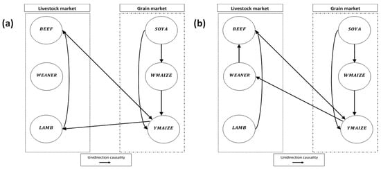
The Toda–Yamamoto causality test was also applied due to the test’s ability to enhance the robustness of causality. The optimal lag order was identified in Table 3 as 2, and the maximum order of integration () was identified as I(1) for all the series. Therefore, the augmented VAR(+) shown in Equation (11) was applied to perform the Toda–Yamamoto causality test by fitting a VAR(3) model, and the results are displayed in Table 12. Lamb carcass prices were identified as Granger causing beef carcass prices, establishing a predictive influence. In turn, beef carcass prices were found to Granger cause yellow maize prices. Additionally, yellow maize prices exhibited Granger causality with live weaner prices, while soybean prices were observed to Granger cause both white and yellow maize prices. Notably, live weaner prices Granger caused beef carcass prices. The findings from Table 12 are summarized in Figure 3b.
Table 12.
Granger causality test based on the Toda–Yamamoto procedure.
Figure 3a,b summarize the VECM and Toda–Yamamoto Granger causality relationships derived from Table 11 and Table 12, respectively. Notably, both graphs revealed similarities in identified causal links among the variables. However, the VECM Granger causality results (Figure 3a) revealed that yellow maize Granger caused lamb carcass prices. In contrast, the Toda–Yamamoto Granger test (Figure 3b) found that yellow maize Granger caused live weaner prices. Furthermore, the Toda–Yamamoto test revealed a causal relationship between live weaner prices and beef carcass prices, whereas the VECM Granger causality test did not find this relationship. Ref. [37] emphasized that relying on VECM for Granger causality tests may lead to biased results due to the pre-testing issues. Recognizing the enhanced robustness of the Toda–Yamamoto procedure, this study emphasized its outcomes.
3.6. Impulse Response Function Analysis
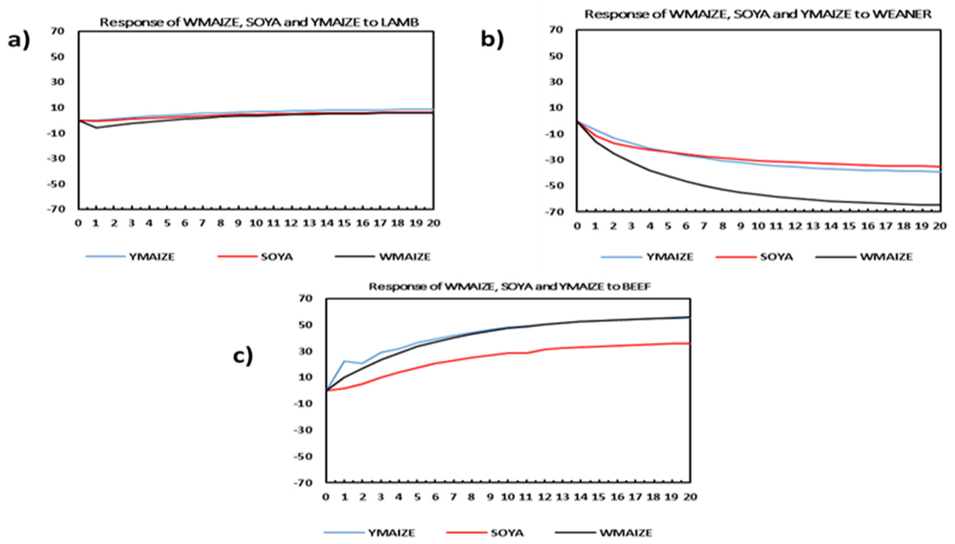
The impulse response analysis in Figure 4 shows a positive reaction of soybean, white maize, and yellow maize prices to shocks in lamb (Figure 4a) and beef carcass prices (Figure 4c), with a more substantial effect from beef carcass prices. Conversely, shocks to live weaner prices (Figure 4b) resulted in a sustained negative influence on grain prices, particularly affecting white maize, which significantly declined.
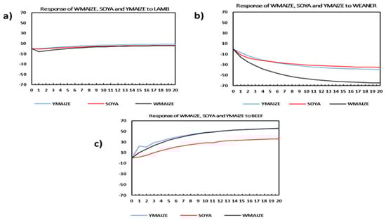
Figure 4.
Impulse response analysis of grain variables in the livestock industry. Source: authors’ compilation. Note: (a,b,c) represent the responses of white maize, soybean, and yellow maize prices to shocks in lamb carcass, live weaner, and beef carcass prices, respectively.
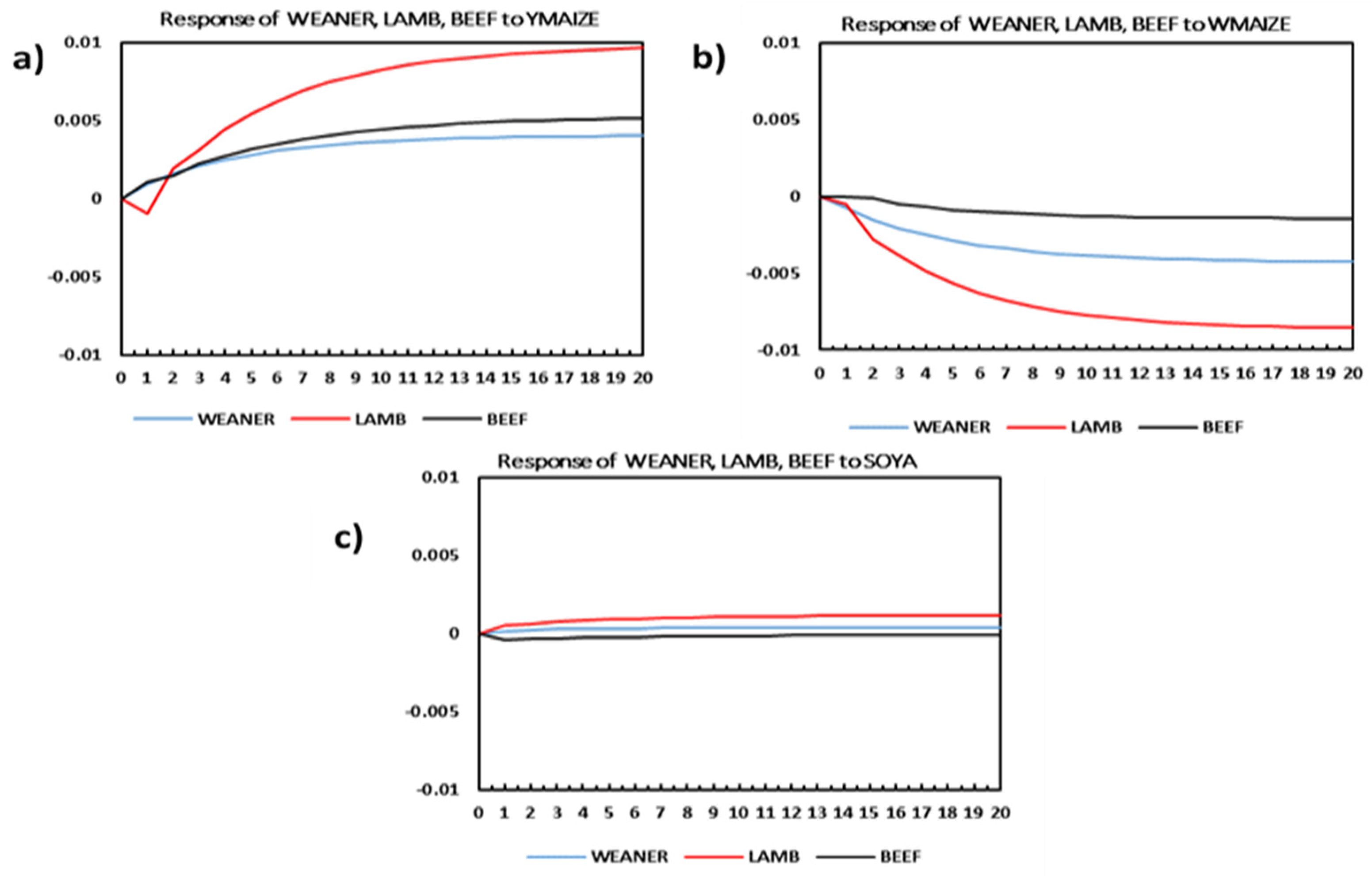
Figure 5 illustrates the impact of standard shocks to key grain prices on livestock markets. A shock to yellow maize prices (Figure 5a) triggered an immediate and sustained increase in live weaner and beef carcass prices, while lamb carcass prices initially decreased before increasing in subsequent weeks. Conversely, a shock to white maize prices (Figure 5b) induced a simultaneous adverse reaction in all three livestock prices, with lamb carcass prices experiencing a notable decline. A shock to soybean prices (Figure 5c) resulted in a modest increase in weaner and lamb prices and a minor decrease in beef carcass prices.
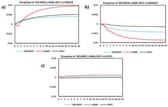
Figure 5.
Impulse response analysis of the livestock industry on the grain industry. Source: authors’ compilation. Note: (a,b,c) represent the responses of lamb carcass, live weaner, and beef carcass prices to shocks in white maize, soybean, and yellow prices, respectively.
3.7. Forecast Error Variance Decomposition
Impulse response functions and forecast error variance decomposition (FEVD) are complementary tools in VECM analysis. Impulse response functions assist in measuring the dynamic response of variables due to shocks in the system. At the same time, FEVD quantifies the contribution of these shocks to the overall variability in each variable. Specifically, FEVD measures the fraction of the forecast error variance of an endogenous variable attributed to shocks to itself or other endogenous variables. Table 13 shows the FEVD results of yellow maize, white maize, and soybean prices, while Table 14 specifically examines the FEVD of live weaner prices and carcass prices for lamb and beef.
Table 13.
Variance decomposition of live weaner, beef, and lamb impulses on maize and soya prices.
Table 14.
Variance decomposition of maize and soybean impulses on live weaner, beef, and lamb prices.
In Table 13, the FEVD for yellow maize highlights a significant impact of its own shocks, particularly in period 1 (99.924%), diminishing over the forecast horizon. Initially, livestock variables minimally contributed to the FEVD of yellow maize, but by period 20, beef carcass prices showed the highest contribution of 15.761%. White maize began with a notable FEVD at period 1 (52.868%), indicating a substantial contribution from factors outside the white maize market. Livestock variables exhibited minimal effects initially but gradually impacted the FEVD of white maize, with contributions from live weaner, lamb, and beef carcass prices at 19.922%, 10.251%, and 1.018%, respectively, in period 20. Soybean prices exhibited increasing self-dependency (82.845% to 87% from periods 1 to 20), contrasting with the decreasing FEVD values observed for white and yellow maize prices. The livestock variables minimally impacted the FEVD of soybean prices.
Table 14 indicates high self-dependency in the forecast error variance decomposition (FEVD) of live weaner prices, starting at 100% and gradually diminishing to 90.088% by period 20. Grain variables had minimal impact, with white maize contributing the most at 9.071% in period 20. For beef carcass prices, there was initial high self-dependency. However, beef carcass prices’ contribution towards their own FEVD decreased to 50.714% by period 20. Yellow maize prices had the highest contribution of the FEVD of lamb carcass prices, reaching 23.146% at period 20. Lamb carcass prices displayed a significant initial self-dependency (98.666% in period 1), gradually decreasing to 83.510% by period 20. White maize prices became more influential, contributing 13.084% in period 20 to the FEVD of lamb carcass prices, while soybean had a minimal effect.
4. Discussion
In this article, using the Johansen cointegration test, it was established that there is a long-run relationship among the study variables. This contrasts with Musunuru’s [41] findings, where the author observed no long-run relationship between grain and meat prices, only identifying short-run relationships. This disparity underscores how commodity market dynamics can vary across different countries or regions.
Furthermore, the consistently low error correction terms obtained from the VECM estimates (Table 7) imply that deviations from the long-run equilibrium take time to correct in the short term. Our study’s identification of consistently low error correction terms aligns with the research conducted by De Zhou and Koemle [42], who found comparable slow adjustment dynamics in China’s hog and feed markets. Our study focused on live weaner prices as our primary livestock variable, whereas De Zhou and Koemle’s [42] research centered on China’s hog market. Despite the difference in livestock species, our comparative analysis highlights different dynamics between live animal variables. De Zhou and Koemle’s [42] findings suggest an 11-month adjustment period for hog prices, whereas our study revealed a 3.5-month correction period for live weaner prices in South Africa. Additionally, slow adjustments were also observed in other livestock markets. For instance, Ajjan et al. [43] found that the maize and poultry market in India is cointegrated, with the highest speed of adjustment found in their study for egg prices at 12% per week, translating roughly to 2 months to fully correct a deviation from the long-run equilibrium. This comparison further underscores broader patterns in market dynamics across livestock sectors and geographical regions.
Moreover, our examination revealed differing rates of adjustment among our study variables, suggesting an asymmetrical transmission of prices within South Africa’s grain and livestock sector. This parallels De Zhou and Koemle’s [42] research, which similarly identified varying adjustment speeds across different markets in China, encompassing hogs, maize, and soybeans. The variations in adjustment speeds across different variables suggest potential inefficiencies within the grain and livestock markets, warranting further investigation into the factors driving these differences.
In addition, our study confirmed a long-term positive relationship between yellow maize and soybean prices and live weaner prices. This finding is similar to Ozdemir’s [44] observations regarding the significant influence of grain feed prices on the beef market in the U.S. Additionally, our analysis resembles the insights of Wang et al. [45] in China, which highlight the impact of minor increases in hog prices on breeding costs and overall hog prices. Moreover, Tejeda and Goodwin’s [46] research underscores the broader implications of input price increases on livestock and food prices, a concept further supported by our findings. Particularly, our impulse response functions demonstrate the direct effect of South African yellow maize market shocks on livestock prices. Thus, although each study offers unique insights, our findings contribute to a more comprehensive understanding of the universal importance of grain prices in shaping livestock markets, particularly emphasizing the significance of yellow maize and soybean prices in our analysis.
Our study results also revealed a positive long-run relationship between beef carcass prices and live weaner prices. This finding is supported by Oosthuizen [47], who suggested that high beef carcass prices incentivize feedlots to purchase more weaners for feeding and eventual slaughter. The second cointegration equation (Equation (13)) further supports this relationship by indicating that as beef and lamb carcass prices increase over the long run, yellow maize prices also increase. This suggests that higher carcass prices stimulate demand for live weaners, subsequently leading to increased demand for feed commodities like yellow maize. Spies [48] also observed significant price transmissions downward from retail to producer levels in the South African beef value chain, aligning with our findings on the influence of beef carcass prices on live weaners. The findings from our study, complemented by the studies of Oosthuizen [47] and Spies [48], contribute to a deeper understanding of how pricing dynamics operate within the livestock sector.
Furthermore, the long-term positive impact of beef and lamb carcass prices on yellow maize prices aligns with the findings of Seok et al. [49], who observed a significant influence of beef prices on yellow maize prices in the U.S. Seok et al. [49] attributed this connection to the substantial size of the beef market in the U.S., which exerts significant demand pressure on yellow maize prices. Marsh [50] also observed that the yellow maize sector in the U.S. benefits from increased demand in the beef retail market, leading to heightened demand for animal feeds. South Africa is suspected to share a similar situation to the U.S. regarding a significant portion of the demand for yellow maize originating from the livestock industry. According to the NAMC [3], the livestock sector in South Africa accounts for approximately 70% of the demand for yellow maize and 86% of the demand for soybeans. Considering our results and the statistics provided by NAMC [3], it appears that the South African beef market exercises price leadership in the South African yellow maize market. These insights indicate the intricate dynamics between livestock and grain markets, highlighting the lasting influence of livestock prices on yellow maize prices in both the U.S. and South Africa.
Also notable from the second cointegrating equation (Equation (13)) is that an increase in live weaner prices has a negative effect on yellow maize prices. Although the beef carcass market plays a dominant role in the South African yellow maize market, it seems that fluctuations in weaner calf prices also play a role in shaping this relationship. Marsh [50] noted that North America’s 2003 bovine spongiform encephalopathy (BSE) outbreaks negatively affected feeder cattle, slaughter cattle, and corn markets. Though not explicitly mentioned by Marsh [50], it can be inferred that BSE reduced the number of live weaners, consequently diminishing the demand for yellow maize. This inference supports our finding that higher live weaner prices negatively impact yellow maize prices, as reduced demand corresponds with weaner calf price fluctuations. South Africa’s livestock market is susceptible to disease outbreaks such as foot and mouth disease (FMD), which detrimentally affects industry productivity [51,52,53]. Therefore, our findings and those of Marsh [50] highlight the critical importance of understanding livestock–grain market dynamics, external factors like disease outbreaks, and informed decision-making for enhancing market stability and resilience in South Africa’s agricultural sector.
The error correction term for soybean prices lacks statistical significance, indicating that deviations from long-run equilibrium do not significantly affect soybean prices. Our causality tests confirmed that other variables do not affect soybean prices significantly. Additionally, impulse response function analysis suggests minimal impact of soybean market shocks on livestock prices. Our results are comparable to those of Fiszeder and Orzeszko [54], who similarly observed limited causal relationships involving soybean prices relative to the livestock market in the U.S. The isolation of soybean prices from livestock variables in our study may be attributed to unique factors in the South African livestock and grain markets. Firstly, according to AFMA [2], soybeans constitute only about 15% of the total feed content in South Africa, suggesting its limited direct impact on overall livestock production. Similarly, Fiszeder and Orzeszko [54] attributed the lack of causal effects between livestock market and soybean price to the fact that cattle are not a huge consumer of soybeans, and therefore such a result is expected. The low usage of soybeans in livestock feeds is attributed to soybean’s status as one of the most expensive protein sources in feed rations [55]. Secondly, South Africa’s soybean production has experienced significant growth in recent years, accompanied by a substantial increase in soybean processing capacity. However, the South African soybean market can be considered to be in its infancy, with connections between the soybean and livestock industries yet to reach full maturity. As production stabilizes and market dynamics evolve, more significant interactions may emerge in the future.
Also notable from the results is the low FEVD of white maize due to its past shocks, suggesting that external factors significantly influence South Africa’s white maize market. Previous studies have identified various external factors as key drivers of white maize prices in South Africa [24,56,57,58]. Therefore, our results support the notion of the importance of considering external influences when analyzing white maize price dynamics in South Africa.
Our study, employing the Toda–Yamamoto causality test, revealed significant short-run relationships, particularly within the grain market, where all causal links converge on yellow maize. This aligns with the statistics provided by the AFMA [2] highlighting yellow maize’s dominant role in South Africa’s livestock feed sector. Importantly, our findings underscore the pivotal role of yellow maize as the sole grain variable influenced by the livestock market, thus serving as a crucial bridge between the grain and livestock sectors, a perspective also emphasized by the AFMA’s [2] data. Interestingly, our results parallel those of Tegle [59], who similarly found limited causal relationships between grain and livestock variables but identified strong causal relationships among various grains. However, our study diverges from Tegle’s [59] findings in one key aspect. Whereas Tegle [59] found that other grain variables also impact soybeans, our results indicate that none of our study variables influenced soybeans. Overall, our causality results underscore pivotal role of yellow maize in facilitating market linkages between the grain and livestock sectors in South Africa.
Furthermore, elaborating on the Toda–Yamamoto causality test results in the livestock market, lamb carcass and live weaner prices were found to Granger cause beef carcass prices, while beef carcass prices influenced yellow maize prices in the grain market. The unidirectional causal effect from lamb to beef carcass prices is consistent with the findings of Lawrence et al. [60] on cross-commodity price transmission between beef and mutton in the U.S. Pozo and Schroeder [61] observed that consumer preferences and disposable income also drive the substitution effect between beef and lamb consumption. Ogundeji and Maré [62] also noted that the substitution between beef and lamb particularly occurs in market situations with relatively high beef prices. Our Toda–Yamamoto causality test also identified a unidirectional causal relationship from live weaner prices to beef carcass prices, consistent with the upward causal relationships observed in the South African beef value chain by spies [48].
5. Conclusions
This study has shed light on the complex interactions between South Africa’s livestock and grain markets, uncovering noteworthy findings with important implications for policymakers and stakeholders. Specifically addressing the research question posed in the introduction, our research has provided a comprehensive examination of the dynamics of price transmissions between these markets, offering valuable insights for policymakers and stakeholders to consider when addressing challenges and capitalizing on opportunities within the agricultural sector. Firstly, the confirmation of a long-run relationship among the study variables underscores the interconnectedness within the South African grain and livestock markets. Additionally, the observed consistently low error correction terms highlight the slow adjustment dynamics, indicative of asymmetric price transmission. To address these findings, policymakers should prioritize the implementation of measures aimed at stabilizing both grain and livestock markets. Specifically for the grain market, regulations could focus on ensuring fair pricing mechanisms, promoting transparency in trading, and preventing market manipulation. Similarly, for the livestock market, policies could be implemented to address issues such as animal welfare standards, disease control measures, and fair-trade practices. By fostering market resilience and mitigating the impact of asymmetries in price transmission, these measures can enhance the overall stability and sustainability of the South African agricultural sector, ensuring more robust market conditions for stakeholders across the value chain.
Secondly, the observation regarding the significant influence of external factors on South Africa’s white maize market highlights a critical concern, especially considering its status as a staple food source for South Africa and other SADC members reliant on imports from South Africa. Given the global predominance of yellow maize production and the limited availability of white maize, South Africa could face challenges in securing reliable sources for white maize imports during shortages and drought. Policymakers need to strategize to increase white maize hectares without compromising yellow maize production, considering the country’s significant yellow maize exports. Balancing these priorities is essential to ensure food security and stability in South Africa and among other African countries reliant on South Africa.
Thirdly, our findings indicate that soybean prices in South Africa are relatively insulated from the influence of other study variables, as evidenced by the lack of statistical significance in the error correction term and causality test results. The minimal impact of soybean market shocks on livestock prices further underscores this independence. These findings emphasize the importance for stakeholders to acknowledge the emerging nature of the soybean industry in South Africa. These results suggest a need for stakeholders to explore diversification opportunities in livestock feed sources. By reducing dependency on specific inputs like soybeans, the livestock market can enhance its resilience and mitigate risks associated with fluctuations in the emerging South African soybean market.
In addition, it might be noteworthy for policymakers to also encourage collaboration between the grain and livestock sectors in South Africa for fostering better market understanding, facilitating policy formulation, and enhancing overall agricultural sustainability. Although Grain South Africa (Grain SA) and the Red Meat Producers Organization (RPO) hold separate annual congress meetings for their respective members, there is a pressing need to encourage collaborative efforts between these sectors to maximize the effectiveness of policymaking and industry development initiatives. Therefore, policymakers should consider facilitating a collaborative effort between these two sectors annually, as they are highly interrelated, as highlighted by our results.
Acknowledging certain limitations, this study highlights areas for future consideration. Firstly, the analysis, conducted within a VAR/VECM framework, requires further robustness to address potential endogeneity issues arising from policy changes or exogenous shocks affecting grain and livestock markets. Secondly, our reliance on economic variables overlooks influential factors such as environmental impact and government policies, which could significantly influence price dynamics. Lastly, our focus on price relationships neglects other critical factors, such as supply–demand dynamics, technological advancements, and international trade policies, which could enhance the comprehensiveness of our understanding of the grain–livestock market dynamics in South Africa. Future research should strive to incorporate these factors for a more comprehensive understanding of market dynamics. Additionally, future research should consider extending the time frame beyond the five-year period analyzed in this study. A more extensive time frame could further contribute to our understanding of the grain–livestock dynamics in South Africa by capturing long-term trends and fluctuations.
Author Contributions
Conceptualization, M.A.M. and B.D.J.; methodology, M.A.M. and B.D.J.; validation, M.A.M. and B.D.J.; formal analysis, M.A.M. and B.D.J.; investigation, M.A.M. and B.D.J.; data curation, M.A.M. and B.D.J. writing—original draft preparation, M.A.M. and B.D.J.; writing—review and editing, M.A.M. and B.D.J.; visualization, M.A.M. and B.D.J. All authors have read and agreed to the published version of the manuscript.
Funding
This research received no external funding.
Institutional Review Board Statement
Not applicable.
Informed Consent Statement
Not applicable.
Data Availability Statement
Data available on request from the authors.
Conflicts of Interest
The authors declare no conflicts of interest.
References
- DALRRD. Abstract of Agricultural Statistics 2023; Department of Agriculture, Land Reform and Rural Development: Pretoria, Switchboard, 2023. Available online: https://www.dalrrd.gov.za/images/Branches/Economica%20Development%20Trade%20and%20Marketing/Statistc%20and%20%20Economic%20Analysis/statistical-information/abstract-2023.pdf (accessed on 12 January 2024).
- Animal Feed Manufacturers Association. AFMA Industry Statistics; Australian Financial Markets Association Limited: Sydney, NSW, Australia, 2024; Available online: https://www.afma.co.za/industry-statistics/ (accessed on 7 February 2024).
- NAMC. South African Grain and Oilseeds Supply & Demand Estimates; National Agricultural Marketing Council: Pretoria, South Africa, 2024; Available online: https://www.namc.co.za/category/research-publications/supply-demand-estimates/ (accessed on 12 January 2024).
- Gardebroek, C.; Hernandez, M.A.; Robles, M. Market interdependence and volatility transmission among major crops. Agric. Econ. 2015, 47, 141–155. [Google Scholar] [CrossRef]
- Fasanya, I.O.; Odudu, T.F. Modeling return and volatility spillovers among food prices in Nigeria. J. Agric. Food Res. 2020, 2, 100029. [Google Scholar] [CrossRef]
- Balcilar, M.; Bekun, F.V. Spillover dynamics across price inflation and selected agricultural commodity prices. J. Econ. Struct. 2020, 9, 2. [Google Scholar] [CrossRef]
- Jena, P.K. Commodity market integration and price transmission: Empirical evidence from India. Theor. Appl. Econ. 2016, 23, 283–306. [Google Scholar]
- Elgammal, M.M.; Ahmed, W.M.; Alshami, A. Price and volatility spillovers between global equity, gold, and energy markets prior to and during the COVID-19 pandemic. Resour. Policy 2021, 74, 102334. [Google Scholar] [CrossRef]
- Kang, S.H.; McIver, R.; Yoon, S.-M. Dynamic spillover effects among crude oil, precious metal, and agricultural commodity futures markets. Energy Econ. 2017, 62, 19–32. [Google Scholar] [CrossRef]
- Garcia-Jorcano, L.; Sanchis-Marco, L. Spillover effects between commodity and stock markets: A SDSES approach. Resour. Policy 2022, 79, 102926. [Google Scholar] [CrossRef]
- Sirohi, J.; Hloušková, Z.; Bartoňová, K.; Malec, K.; Maitah, M.; Koželský, R. The Vertical Price Transmission in Pork Meat Production in the Czech Republic. Agriculture 2023, 13, 1274. [Google Scholar] [CrossRef]
- Ben Haddad, H.; Mezghani, I.; Gouider, A. The Dynamic Spillover Effects of Macroeconomic and Financial Uncertainty on Commodity Markets Uncertainties. Economies 2021, 9, 91. [Google Scholar] [CrossRef]
- Hung, N.T. Oil prices and agricultural commodity markets: Evidence from pre and during COVID-19 outbreak. Resour. Policy 2021, 73, 102236. [Google Scholar] [CrossRef]
- Alam, K.; Tabash, M.I.; Billah, M.; Kumar, S.; Anagreh, S. The Impacts of the Russia–Ukraine Invasion on Global Markets and Commodities: A Dynamic Connectedness among G7 and BRIC Markets. J. Risk Financ. Manag. 2022, 15, 352. [Google Scholar] [CrossRef]
- Fang, Y.; Shao, Z. The Russia-Ukraine conflict and volatility risk of commodity markets. Financ. Res. Lett. 2022, 50, 103264. [Google Scholar] [CrossRef]
- Just, M.; Echaust, K. Dynamic spillover transmission in agricultural commodity markets: What has changed after the COVID-19 threat? Econ. Lett. 2022, 217, 110671. [Google Scholar] [CrossRef]
- Kumar, S.; Jain, R.; Balli, F.; Billah, M. Interconnectivity and investment strategies among commodity prices, cryptocurrencies, and G-20 capital markets: A comparative analysis during COVID-19 and Russian-Ukraine war. Int. Rev. Econ. Financ. 2023, 88, 547–593. [Google Scholar]
- Alemu, Z.; Ogundeji, A. Price transmission in the South African food market. Agrekon 2010, 49, 433–445. [Google Scholar] [CrossRef]
- Mkhabela, T.; Nyhodo, B. Farm and Retail Prices in the South African Poultry Industry: Do the Twain Meet? Int. Food Agribus. Manag. Rev. 2011, 14, 127–146. [Google Scholar]
- Lombard, H.L. Price Transmission in the Beef Value Chain—The Case of Bloemfontein, South Africa. Master’s Thesis, University of the Free State, Bloemfontein, South Africa, 2015. [Google Scholar]
- Mosese, D. Analysis of Vertical Price Transmission in the South African Potato Markets. Master’s Thesis, University of Limpopo, Polokwane, South Africa, 2020. [Google Scholar]
- Louw, M.; Meyer, F.; Kirsten, J. Vertical price transmission and its inflationary implications in South African food chains. Agrekon 2017, 56, 110–122. [Google Scholar] [CrossRef]
- Kirsten, J.F. The Political Economy of Food Price Policy in South Africa. In Food Price Policy in an Era of Market Instability: A Political Economy Analysis; United Nations University World Institute for Development Economics Research: Helsinki, Finland, 2012; pp. 407–430. [Google Scholar]
- Abidoye, B.O.; Labuschagne, M. The transmission of world maize price to South African maize market: A threshold cointegration approach. Agric. Econ. 2013, 45, 501–512. [Google Scholar] [CrossRef]
- Pierre, G.; Kaminski, J. Cross country maize market linkages in Africa: Integration and price transmission across local and global markets. Agric. Econ. 2018, 50, 79–90. [Google Scholar] [CrossRef]
- Mokumako, T.; Baliyan, S.P. Transmission of South African maize prices into Botswana markets: An econometric analysis. Int. J. Agric. Mark. 2016, 3, 119–128. [Google Scholar]
- Myers, R.J.; Jayne, T.S. Multiple-regime spatial price tranmission with an application to maize markets in Southern Africa. Am. J. Agric. Econ. 2012, 94, 174–188. [Google Scholar]
- Mphateng, M.A. Spatial Price Transmission and Market Inegration Analysis: The Case of Wheat Market in South Africa, 2010–2019. Master’s Thesis, University of Limpopo, Polokwane, South Africa, 2022. [Google Scholar]
- Ramoroka, P.; Muchopa, C.L. Inter-commodity Price Transmission between Maize and Wheat in South Africa. Int. J. Econ. Financ. Issues 2022, 12, 57–63. [Google Scholar] [CrossRef]
- StataCorp. Stata Statistical Software: Release 15; StataCorp LLC: College Station, TX, USA, 2017. [Google Scholar]
- Badaoui, F.; Bouhout, S.; Amar, A.; Khomsi, K. Modelling of Leishmaniasis Infection Dynamics: A Comparative Time Series Analysis with VAR, VECM, Generalized Linear and Markov Switching Models. Eng. Proc. 2023, 39, 38. [Google Scholar]
- Dickey, D.A.; Fuller, W.A. Likelihood Ratio Statistics for Autoregressive Time Series with a Unit Root. Econometrica 1981, 49, 1057–1072. [Google Scholar] [CrossRef]
- Dickey, D.A.; Fuller, W.A. Distribution of the Estimators for Autoregressive Time Series with a Unit Root. J. Am. Stat. Assoc. 1979, 74, 427. [Google Scholar] [CrossRef]
- Engle, R.F.; Granger, C.W.J. Co-Integration and Error Correction: Representation, Estimation, and Testing. Econometrica 1987, 55, 251–276. [Google Scholar] [CrossRef]
- Johansen, S. Statistical analysis of cointegration vectors. J. Econ. Dyn. Control 1988, 12, 231–254. [Google Scholar]
- Johansen, S. Estimation and Hypothesis Testing of Cointegration Vectors in Gaussian Vector Autoregressive Models. Econometrica 1991, 59, 1551–1580. [Google Scholar] [CrossRef]
- Levendis, J.D. Time series econometrics learning through replication. In Introductory Econometrics: A Practical Approach; Springer: Berlin/Heidelberg, Germany, 2018; 271p. [Google Scholar]
- Granger, C.W.J. Investigating Causal Relations by Econometric Models and Cross-spectral Methods. Econometrica 1969, 37, 424–438. [Google Scholar] [CrossRef]
- Toda, H.Y.; Yamamoto, T. Statistical inference in vector autoregressions with possibly integrated processes. J. Econom. 1995, 66, 225–250. [Google Scholar] [CrossRef]
- Lüutkepohl, H.; Saikkonen, P.; Trenkler, C. Maximum eigenvalue versus trace tests for the cointegrating rank of a VAR process. Econ. J. 2001, 4, 287–310. [Google Scholar] [CrossRef]
- Musunuru, N. Causal relationship between grain, meat prices and exchange rates. Int. J. Food Agric. Econ. 2017, 5, 1–10. [Google Scholar]
- De, Z.; Koemle, D. Price transmission in hog and feed markets of China. J. Integr. Agric. 2015, 14, 1122–1129. [Google Scholar]
- Ajjan, N.; Murugananthi, D.; Raveendaran, N. An Econometric Analysis of Maize and Poultry Market Integration in India. Madras Agric. J. 2012, 99, 397–402. [Google Scholar] [CrossRef]
- Ozdemir, D. Cyclical causalities between the U.S. wholesale beef and feed prices: A Markov-switching approach. Econ. Bus. Lett. 2020, 9, 135–145. [Google Scholar]
- Wang, G.; Si, R.; LI, C.; Zhang, G.; Zhu, N. Asymmetric price transmission effect of corn on hog: Evidence from China. Agric. Econ. 2018, 64, 186–196. [Google Scholar] [CrossRef]
- Tejeda, H.A.; Goodwin, B.K. Price volatility, nonlinearity, and asymmetric adjustments in corn, soybean, and cattle markets: Implications of ethanol-driven (market) shocks. In Proceedings of the NCCC-134 Applied Commodity Price Analysis, Forecasting, and Market Risk Management, St. Louis, MI, USA, 20–21 April 2009. No 1315-2016-102674. [Google Scholar]
- Oosthuizen, P.L. The Profit-Maximising Feeding Period for Different Cattle Breeds. Master’s Thesis, University of the Free State, Bloemfontein, South Africa, 2016. [Google Scholar]
- Spies, D.C. Analysis and Quantification of the South African Red Meat Value Chian. Ph.D. Thesis, University of the Free State, Bloemfontein, South Africa, 2011. [Google Scholar]
- Seok, J.H.; Kim, G.; Kim, S. Causal Relationship among Bioethanol Production, Corn Price, and Beef Price in the U.S. Environ. Resour. Econ. Rev. 2018, 27, 521–544. [Google Scholar]
- Marsh, J.M. Cross-Sector Relationships between the Corn Feed Grains and Livestock and Poultry Economies. J. Agric. Resour. Econ. 2007, 32, 93–114. [Google Scholar]
- Roberts, L.C.; Fosgate, G.T. Stakeholder perceptions of foot-and-mouth disease control in South Africa. Prev. Veter-Med. 2018, 156, 38–48. [Google Scholar] [CrossRef]
- Fanadzo, M.; Ncube, B. Review: Challenges and opportunities for revitalising smallholder irrigation schemes in South Africa. Water SA 2018, 44, 436–447. [Google Scholar] [CrossRef]
- Sirdar, M.M.; Fosgate, G.T.; Blignaut, B.; Mampane, L.R.; Rikhotso, O.B.; Du Plessis, B.; Gummow, B. Spatial distribution of foot -and-mouth disease (FMD) outbreaks in South Africa (2005–2016). Trop. Anim. Health Prod. 2021, 53, 1–12. [Google Scholar]
- Fiszeder, P.; Orzeszko, W. Nonlinear Granger causality between grains and livestock. Agric. Econ. 2018, 64, 328–336. [Google Scholar] [CrossRef]
- Parrini, S.; Aquilani, C.; Pugliese, C.; Bozzi, R.; Sirtori, F. Soybean Replacement by Alternative Protein Sources in Pig Nutrition and Its Effect on Meat Quality. Animals 2023, 13, 494. [Google Scholar] [CrossRef]
- Monk, M.; Jordaan, H.; Grové, B. Factors affecting the price volatility of July futures contracts for white maize in South Africa. Agrekon 2010, 49, 446–458. [Google Scholar] [CrossRef]
- Sayed, A.; Auret, C. Volatility transmission in the South African white maize futures market. Eurasian Econ. Rev. 2019, 10, 71–88. [Google Scholar] [CrossRef]
- Auret, C.J.; Schmitt, C.C. An Explanatory Model of South African White Maize Futures Prices. Stud. Econ. Econ. 2008, 32, 103–131. [Google Scholar] [CrossRef]
- Tegle, A. An Explorative Study of Grain and Meat Price Relationships. Master’s Thesis, Norwegian University of Life Sciences, As, Norway, 2013. [Google Scholar]
- Lawrence, J.D.; Mintert, J.R.; Anderson, J.D. Feed grains and livestock: Impacts on meat supplies and prices. Choices 2008, 23, 11–15. [Google Scholar]
- Pozo, F.P.; Schroeder, T.C. Price and Volatility Spillover between Livestock and Related Commodity Markets. In Proceedings of the Agricultural & Applied Economics Association’s 2012 AAEA Annual Meeting, Seattle, WA, USA, 12–14 August 2012; pp. 12–14. [Google Scholar]
- Ogundeji, A.; Maré, F. Analysis of price transmission in the beef value chain using a calculated retail carcass price. Agrekon 2020, 59, 144–155. [Google Scholar] [CrossRef]

Disclaimer/Publisher’s Note: The statements, opinions and data contained in all publications are solely those of the individual author(s) and contributor(s) and not of MDPI and/or the editor(s). MDPI and/or the editor(s) disclaim responsibility for any injury to people or property resulting from any ideas, methods, instructions or products referred to in the content. |
© 2024 by the authors. Licensee MDPI, Basel, Switzerland. This article is an open access article distributed under the terms and conditions of the Creative Commons Attribution (CC BY) license (https://creativecommons.org/licenses/by/4.0/).