Developing a Data-Driven AI Model to Enhance Energy Efficiency in UK Residential Buildings

Abstract

Residential buildings contribute 30% of the UK’s total final energy consumption. However, with less than one percent of its housing stock being replaced annually, retrofitting existing homes has significant importance in meeting energy-efficiency targets. Consequently, many physics-based and data-driven models and tools have been developed to analyse the effects of retrofit strategies from various points of view. This paper aims to develop a data-driven AI model that predicts buildings’ energy performance based on their features under various retrofit scenarios. In this context, four different machine learning models were developed based on the EPC (Energy Performance Certificate) dataset for residential buildings and standard assessment procedure (SAP) guidelines in the UK. Additionally, an interface was designed that enables users to analyse the effect of different retrofit strategies on a building’s energy performance using the developed AI models. The results of this study revealed the artificial neural network as the most accurate predictive model, with a coefficient of determination (R²) of 0.82 and a mean percentage error of 11.9 percent. However, some conceptual irregularities were observed across all the models when dealing with different retrofit scenarios. All summary, such tools can be further improved to offer a potential alternative or support to physics-based models, enhancing the efficiency of retrofitting processes in buildings.

1. Introduction

The building sector accounts for the largest share of global total final energy consumption (more than 35 percent), and over 85% of this is allocated to the operational needs of buildings [1]. In response, various energy conservation plans for buildings have been developed to ensure their efficiency and sustainability. In this regard, building energy performance prediction is crucial for implementing energy efficiency plans in buildings, facilitating effective conservation measures that lead to reduced energy consumption.

Energy prediction models can be classified into two different categories: physics-based and data-driven (artificial intelligence) modelling approaches [2]. Physics-based models (e.g., IESEVE, EnergyPlus) utilize physical and thermodynamic laws and require a large set of input data regarding building characteristic details, such as envelope materials and thickness. These models often involve lengthy simulation times and lack flexibility when it comes to making changes to individual variables, making them less suitable for dynamic scenarios.

On the other hand, data-driven models utilize artificial intelligence algorithms (e.g., machine learning algorithms) to discover non-linear relationships between inputs (e.g., building features) and outputs (e.g., annual energy consumption). This capability enables them to learn consumption patterns from historical data, enhancing their predictive accuracy. Hence, many machine learning algorithms, including regression- and classification-based approaches, have been developed to predict building energy consumption, and various studies of different case studies have been conducted to assess the accuracy and effectiveness of these models in estimating buildings’ energy consumption.

Razak et al. [3] conducted a study to utilize ensemble learning classification-based methods including support vector machine (SVM), gradient boosting (GB), and extra trees (ET) to predict residential buildings’ energy performance certificates in the UK. The findings of this study highlighted the better performance of the ET algorithm; however, the accuracy index of all the developed models ranged between 0.56 and 0.64. This study was later extended by [4], in which nine different models including an artificial neural network (ANN), a deep neural network (DNN), and ensemble learning regression-based techniques were developed to predict annual energy consumption (KWh/m²) in residential buildings across the UK. The output of the developed models in this study revealed outstanding results for the deep neural network (DNN), artificial neural network (ANN) support vector machine (SVM), and gradient boosting (GB) algorithms, in which the R² values obtained were higher than 0.9. However, feature importance results in these models show that the output of the model is highly dominated by the “total floor area”, which is in contrast with the fact that the heating system is the most important factor in UK homes’ energy consumption [5].

Another study, conducted in the UK by Seyedzadeh et al. [6] to predict energy performance in non-domestic buildings, used a gradient boost regression tree algorithm to assist in building energy retrofit planning. This study utilized a comprehensive dataset encompassing detailed information on various building features such as air infiltration rates, the characteristics of each building facade, internal gains from equipment, etc. Their model also utilized advanced evolutionary algorithms for optimization, which resulted in less than a 2 percent error.

Some studies have incorporated on-site measurements to develop their ML models. In this regard, Shao et al. [7] utilized an SVM regression algorithm to predict daily energy consumption in a hotel building in China. They created their dataset using daily weather data (temperature and relative humidity) along with on-site measurements of building energy system characteristics. The result of this study revealed outstanding results in terms of R² and mean squared error metrics, which were recorded as 0.94 and 2.2%, respectively. Moreover, Dep et al. [8] found the recurrent neural network (RNN) as the most accurate algorithm in predicting hourly space heating demand for a single-family house located in Switzerland. They utilized 37 sensors to collect data and three different feature selection methods to analyse 41 features and create prediction models. The evaluation of the developed models shows that the RNN has better performance in terms of the R² metric.

Araujo et al. [9] utilized three different ML models, including the GB, ET, and ANN-multilayer perceptron (MLP), based on residential buildings’ EPC database to predict annual heating, cooling, and overall primary energy (KWh/m²) for a case study building. They selected 20 features including general details, construction elements, equipment, and the glazing system of a property. The performance indicator results of the model showed acceptable results for predicting total annual energy in which the R² value obtained was 0.79 for the ET model. On the other hand, its performance was less accurate when predicting annual cooling load, with an R² value not exceeding 0.41.

Pham et al. [10] utilized a random forest (RF) model to predict hourly energy consumption in five educational buildings on 1-step-ahead, 12-step-ahead, and 24-step-ahead bases. They also considered different scenarios to assess the effect of variations in the length of the training data (ranging from 67% to 92%) on the accuracy of the model. The study results showed the model performs acceptably for predicting 1-step-ahead, with mean absolute percentage error (MAPE) values between 5% and 15% for each dataset, and building and changing the model’s training size doesn’t necessarily affect its accuracy.

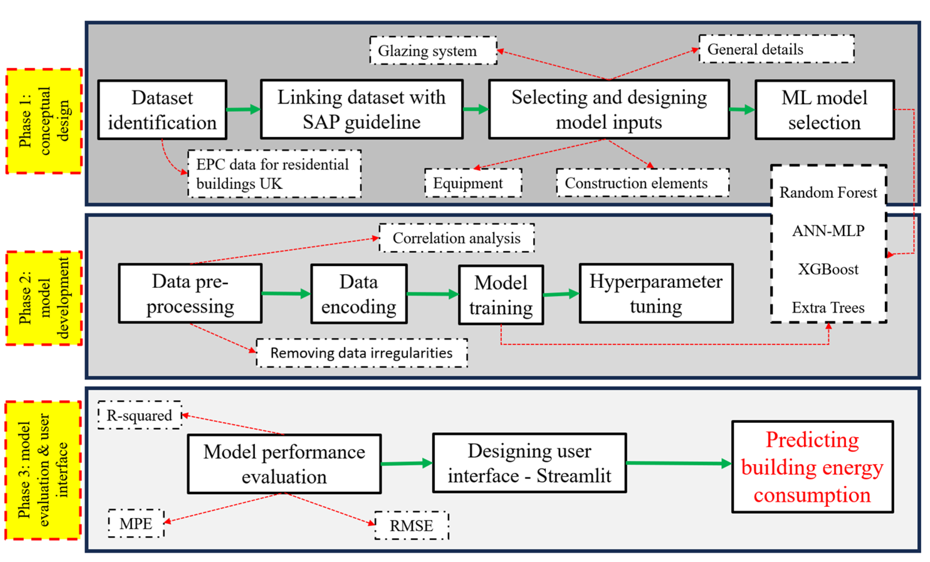
The accuracy of the above-mentioned predictive models is highly dependent on elements such as the extent of the dataset, designed features, target variable, step of prediction, and so on. Moreover, the absence of a user interface to facilitate assessing models’ accuracy from a conceptual point of view was notable, resulting in these studies relying solely on statistical metrics to evaluate the model performance. In order to fill this gap, this research focused on designing models’ features (feature engineering) based on the Standard Assessment Procedure (SAP) and utilizing four machine learning models (including XGB, RF, ET, and ANN-MLP) to develop an AI-based tool that predicts a residential building’s annual energy consumption based on its characteristics. Moreover, an interface will be designed that enables users to input a specific case study building’s characteristics and assess the impact of retrofit strategies on the building’s energy performance, addressing the following key research questions in this study:

• What are the key building features that significantly impact energy consumption in residential buildings, and how do they contribute to the predictive accuracy of machine learning models?
• To what extent can machine learning models effectively capture dynamic changes in energy consumption patterns in residential buildings?
• How do different machine learning algorithms, such as XGB, RF, ET, and ANN-MLP, compare in terms of their effectiveness in predicting residential buildings’ annual energy consumption?

2. Materials and Methods

2.1. Dataset

The study utilized the Energy Performance Certificate dataset for residential buildings in the UK, published by the Department for Levelling Up, Housing and Communities [11]. While the dataset includes information from across the UK, this study specifically focuses on residential buildings in London. This dataset contains detailed numerical and categorical information on building envelope characteristics, energy systems, and estimated annual energy consumption. The data was collected by energy assessors (experts) and follows the Standard Assessment Procedure (SAP), ensuring a comprehensive and standardized assessment of energy performance in residential buildings.

2.2. Data Pre-Processing

Raw data often includes various irregularities, such as missing values, noise, inconsistencies, and redundancies. These anomalies can impact the effectiveness of subsequent learning processes. As a result, the preprocessing step is a common procedure to minimize the impact of any data irregularities on the quality and reliability of subsequent processing steps [12]. It should be noted that in this research, data processing and model development were conducted using the “Sklearn” Python package [13].

To reduce noise and data irregularities in the model, case studies with missing values and outliers were excluded from the dataset. This ensured that the model was built on more accurate observations. For instance, case studies where the floor height was less than 2 m, total annual energy consumption exceeded 600 kWh/m², or the floor area was less than 20 m² were removed from the dataset.

The dataset includes some categorical features, so two common methods for data encoding were utilized in the model: one-hot encoding and label encoding. Each method comes with its own set of pros and cons. While one-hot encoding is effective in representing categorical variables, it can increase dimensionality and complexity, potentially reducing model interpretability; On the other hand, label encoding assigns ordinal meaning to categories. As a result, both methods were applied in each ML model to assess their effectiveness.

Data normalization is another essential pre-processing step which involves the transformation of features in a defined range (within the range of 0 to 1 in this study) so that greater numeric feature values (e.g., total floor area and percentage of low-energy lighting) cannot dominate the model, which will lead to minimizing the bias of these features in the model [14].

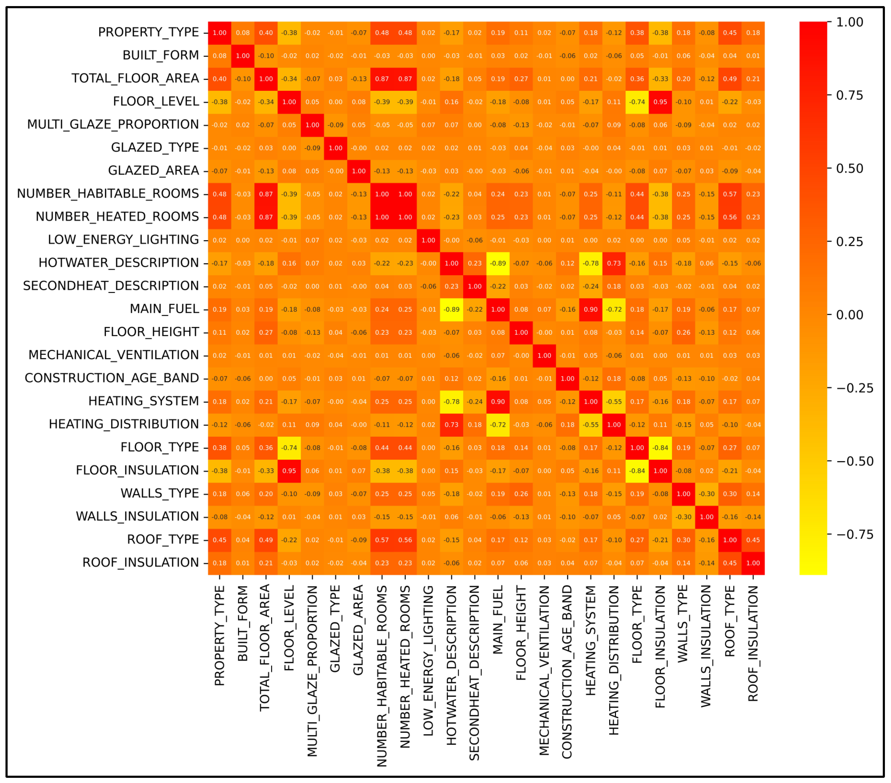
Furthermore, a correlation analysis of the input variables was conducted in this study using a correlation matrix. A correlation matrix is a table (or figure) that represents the correlation coefficient between variables, and a correlation coefficient is a statistical measure that quantifies the relation between two variables. This value ranges between −1 and 1, where 1 indicates a perfect positive correlation, −1 shows a perfect negative correlation, and 0 indicates no correlation. A high correlation between two variables (close to 1 or −1) is an indication that they are highly dependent on each other.

In this regard, the correlation matrix of input variables of the study is shown in Figure 1. So, to reduce the complexity and dimension of the model, whenever the correlation coefficient was calculated at more than 0.8, the redundant variables were removed from the model. For instance, as illustrated in Figure 1, a noticeable correlation is evident between “number of heated rooms” and “number of habitable rooms” with “total floor area”. Consequently, both variables were considered redundant due to this high correlation and were subsequently removed from the model. Overall, correlation analysis eliminated four input variables, resulting in twenty variables remaining in the model. This boosted the model’s simplicity and eliminated unnecessary redundancy, ensuring a more focused and efficient model performance.

2.3. Feature Engineering

A “feature” is an attribute or variable used to describe some aspect of an individual data object, and the general idea of “feature engineering” includes the process of transformation, generation, extraction, selection, analysis, and evaluation of features within a dataset [15]. In this phase of the research, potential features related to both the building energy system and building physics were extracted from the dataset. Additionally, new features were generated based on the descriptions provided for building characteristics in the EPC dataset. Designing new features and their assigned values (or categories) follows the Standard Assessment Procedure (SAP). For instance, using the collected information about wall descriptions, two features were created: “wall type” (including categories like solid brick, cavity wall, and timber frame) and “wall insulation” (with categories such as insulated and as-built). Further details about the selected and designed features can be found in

Table 1. List of designed and selected features (model inputs).

No.	Variable	Type	Range/Categories
1	Property type	Categorical	House, flat, maisonette, bungalow
2	Built form	Categorical	Detached, semi-detached, mid-terrace, end-terrace, enclosed end-terrace, enclosed mid-terrace
3	Glazing type	Categorical	Double, single. secondary, and triple glazing
4	Glazed area	Categorical	Normal, more than typical, less than typical, much more than typical
5	Hot water system	Categorical	Gas boiler, electric immersion, gas multipoint, electric instantaneous, electric boiler, gas instantaneous, air source heat pump
6	Main heating system	Categorical	Gas boiler, electric warm air system, electric room heaters, electric underfloor heating system, electric storage heater, gas-fired warm air system, air source heat pump, electric boiler, gas-fired room heater
7	Secondary heating system	Categorical	Coal/wood heaters, portable electric heaters, portable gas heaters, none
8	Ventilation system	Categorical	Natural, mechanical—extract only, mechanical—supply and extract
9	Construction age band	Categorical	Before 1900, 1900–1929, 1930–1949, 1950–1966, 1967–1975, 1976–1982, 1983–1990, 1991–1995, 1996–2002, 2003–2006, 2007 onwards
10	Heating distribution system	Categorical	Radiators, warm air, room heaters, underfloor system
11	Floor type	Categorical	Solid, premises/dwelling below, to unheated space, suspended, to external air
12	Floor insulation	Categorical	As-built, other dwelling/premises below, insulated
13	Wall type	Categorical	Solid, cavity wall, timber frame
14	Wall insulation	Categorical	As-built, filled cavity, internal insulation, filled cavity plus insulation, external insulation
15	Roof type	Categorical	Dwelling above, pitched roof, flat roof, room roof
16	Roof insulation	Categorical	Another dwelling above, insulated, as-built
17	Floor area	Numerical	20–500 square meters
18	Multi-glazed area of the total glazed area of the property	Numerical	0–100%
19	Floor height	Numerical	2–5 m
20	Percentage of low-energy lighting in the property	Numerical	0–100%

.

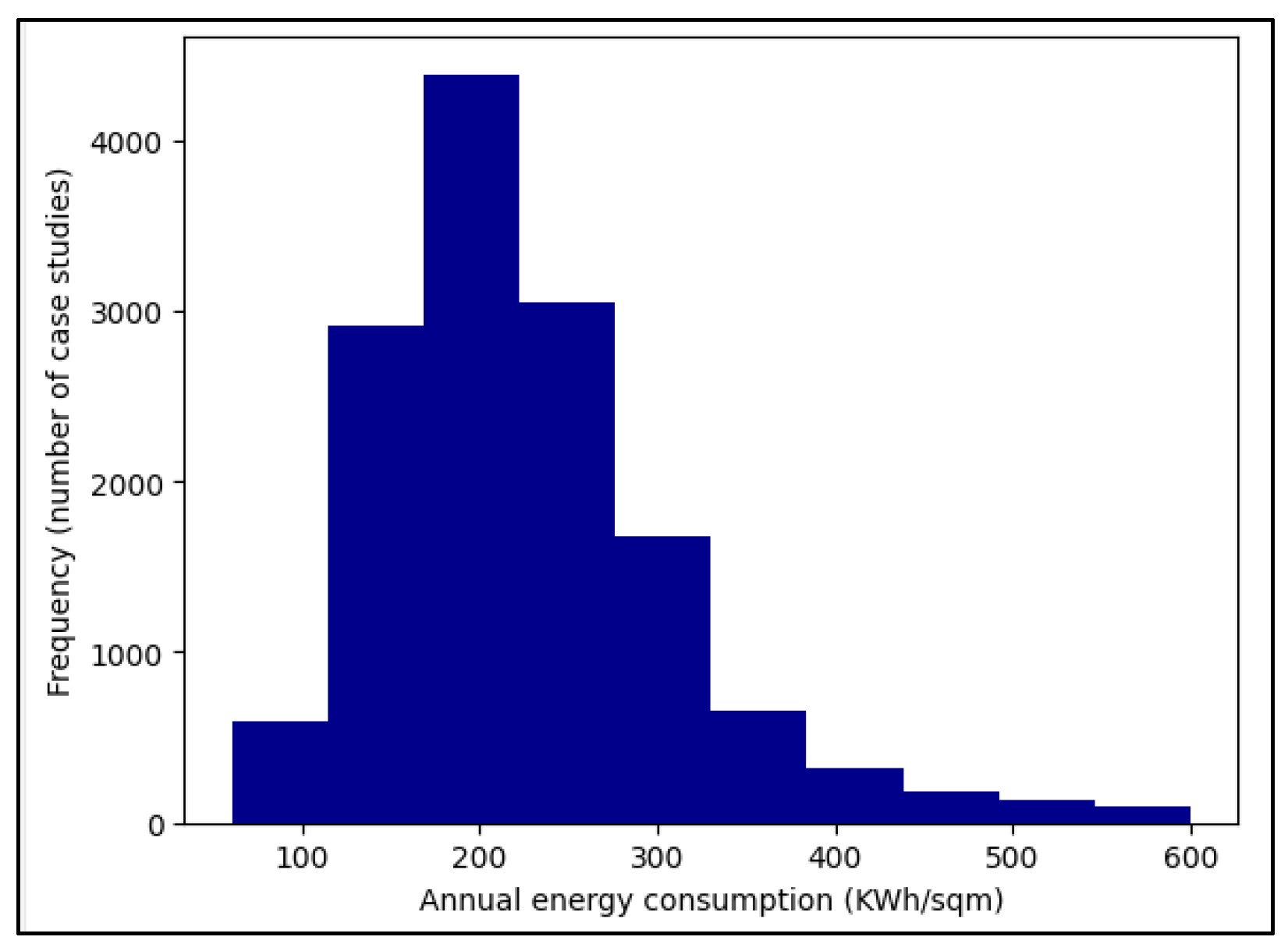
2.4. Data Exploration

An investigation into the 14,000 remaining case studies within the dataset (after data pre-processing) reveals significant trends across various parameters. Regarding property type, the majority comprises flats, accounting for approximately 58% of the dataset, followed by houses at 33%, maisonettes at 7%, and bungalows at 2%. Analysing the heating systems utilized, a clear dominance of gas boilers emerges, representing over 85% of the case studies. Other heating systems such as electric storage and electric room heaters also feature, although to a lesser extent. Notably, only 0.5% of the case studies employ air source heat pumps as their primary heating system. Looking into the construction age bands, nearly 40% of the properties were constructed before 1950, suggesting potential issues with building insulation standards, particularly if they have not been retrofitted. Conversely, only 3.5% of the properties were constructed post-2007, highlighting a modernization gap in the housing stock. Overall, the data shows a central tendency around 200 kWh/m² annual energy consumption, with an average consumption of 226 kWh/m², as shown in Figure 2.

2.5. Model Selection

In this study, a diverse set of ML algorithms was applied to predict building annual energy consumption, including ensemble learning methods as well as an artificial neural network with a multilayer perceptron. Ensemble learning methods integrate individual regressors to improve the predictions. It is accepted that each regressor is likely to learn different aspects of training data. So, combining multiple regressors using ensemble learning can enable the final ML model to search in a wide solution space [16]. In this regard, the ensemble learning methods chosen for this study are random forest (RF), XGBoost (XGB), and extra trees (ET).

These algorithms were chosen based on their accurate performance in the literature for predicting annual building energy consumption, effectiveness in handling both categorical and numerical input features [17], and their robustness in non-linear relationship modelling [16,18]. The following section will provide a highlight of the key features and algorithms employed in the selected ML models.

2.6. Models Theoretical Background

2.6.1. Random Forest

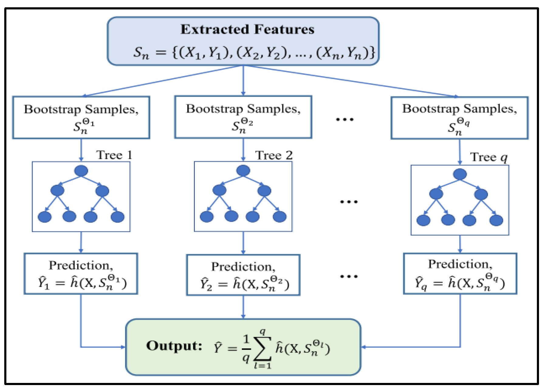
The random forest algorithm is an ensemble learning method that operates by constructing a multitude of decision trees during the training process. A decision tree is a tree-like model where an input is progressively split into subsets based on the values of particular features; and the goal is to create a model that predicts the target variable’s value by learning simple decision rules, inferred from the data features.

A random forest model generates hundreds or even thousands of these decision trees, which act as regression functions on their own, and the final output of the random forest regression is the average of the outputs of all the decision trees. If “X” represents the input vector containing “m” features with $X=\left\{x_1,{ x}_2, ... , x_{m }\right\}$, “Y” represents the output scalar and “S_n” the training set containing “n” samples, which can be expressed as:

$$S_n=\left\{\left(X_1,Y_1\right),\left(X_2,Y_2\right), \dots , \left(X_n,Y_n\right)\right\} X\in {\mathbb{R}}^m, Y\in \mathbb{R}$$

(1)

So, the random forest model can be built by randomly sampling a feature subset for each decision tree, or by randomly sampling a training data subset for each decision tree. This randomly collected sample process is called a “bootstrap”. Each bootstrap sample is obtained by randomly selecting n observations with replacements from the original dataset, and each observation has a probability of 1/n to be selected.

Furthermore, the “bagging” algorithm selects several bootstrap samples $(S_n^{{\theta }_1},S_n^{{\theta }_2},\dots ,S_n^{{\theta }_q})$ in order to build a collection of “q” prediction trees $\widehat{h}\left(X,S_n^{{\theta }_1}\right),\widehat{h}\left(X,S_n^{{\theta }_2}\right)\dots ,\widehat{h}\left(X,S_n^{{\theta }_q}\right)$. The ensemble produces q outputs corresponding to each tree, $\widehat{Y_1}=\widehat{h}\left(X,S_n^{{\theta }_1}\right),\widehat{Y_2}=\widehat{h}\left(X,S_n^{{\theta }_2}\right),\dots ..,\widehat{Y_q}=\widehat{h}\left(X,S_n^{{\theta }_q}\right)$. Then, the aggregation is performed by averaging the outputs of all the trees. Consequently, the estimation $\widehat{Y}$ can be obtained by Equation (1), where $\widehat{Y_1}$ is the output of the l-th tree, and l = 1, 2, …, q [19]:

$$\widehat{Y}=\frac{1}{q} \sum _{l=1}^q\widehat{Y_1}=\frac{1}{q} \sum _{l=1}^q\widehat{h}\left(X,S_n^{{\theta }_1}\right)$$

(2)

The framework for using the random forest regression model is presented in Figure 3.

2.6.2. Extra Trees

Extremely randomized trees (extra trees) is an extension of the random forest algorithm that utilizes additional randomness, not only in the selection of feature subset, but also in the determination of the splitting thresholds for each node. This increased level of randomness aims to create a more diverse set of trees, potentially less likely to overfit a dataset [20].

Although extra trees employs the same principle as random forest, its two key differences are that it splits nodes by choosing cut points fully at random, and it uses the whole learning sample (rather than a bootstrap replica) to grow the trees [20,21]. From a computational point of view, the random splitting process in extra trees (rather than the optimization process for the splitting feature in random forest) is less computationally demanding. As a result, additional randomness in the splitting, robustness against overfitting, and computational efficiency makes extra trees a particularly useful model when dealing with high-dimensional datasets and complex relationships.

2.6.3. XGBoost

Extreme gradient boosting (known as XGBoost) is an end-to-end tree boosting which employs a sparsity-aware algorithm for sparse data and a weighted quantile sketch for tree learning [22]. One of the key factors associated with XGBoost is its scalability, where the system runs ten times faster than existing popular algorithms on a single machine [22]. In this regard, parallel and distributed computing accelerates the learning process, which results in quicker exploration of models.

While random forest builds a set of independent trees and averages their predictions, XGBoost sequentially adds new trees to the ensemble; and each tree aims to improve upon the correction of errors made by the previous trees. A brief description of the XGBoost algorithm for regression along with relevant equations is presented in the following paragraphs.

Given a dataset, $D=\{\left(x_i,y_i\right):i=\mathrm{1,2},\dots ,n x_i\in {\mathbb{R}}^m, y_i\in \mathbb{R}\}$, n observations are obtained, each comprising m features, along with a corresponding variable, y. Let $\widehat{y_i}$ denote the result produced by an ensemble represented by the generalized model as Equation (3). In this equation, $f_k$ represents a regression tree, and $f_k\left(x_i\right)$ denotes the score assigned by the k-th tree to the i-th observation in the dataset. To achieve the function $f_k$, the regularized objective function should be minimized according to Equation (4), where $\mathcal{L}$ is the loss function.

To avoid excessive model complexity, the penalty term Ω is incorporated, as shown in Equation (5). In this equation, T represents the total number of leaf nodes, and ω is the score of each leaf node. γ and λ are controlling factors employed to avoid overfitting [23,24]. Hence, the objective function that is minimized in the j-th iteration is re-written as Equation (6). This function can be simplified using a Taylor polynomial and approximated as Equation (7), where “$g_i$” is the first-order derivative, and “$h_i$” denotes the second-order derivative in Equations (8) and (9).

$$\widehat{y_i}=\varphi \left(x_i\right)={\sum }_{k=1}^K{f}_k\left(x_i\right)$$

(3)

$$\mathcal{L}\left(\varphi \right)={\sum }_{i}l(y_i,\widehat{y_i})+{\sum }_k\mathsf{\Omega }\left(f_k\right)$$

(4)

$$\mathsf{\Omega }\left(f_k\right)=\gamma T+\frac{1}{2}{\lambda \left|\left|\mathsf{\omega }\right|\right|}^2$$

(5)

$${\mathcal{L}}^j={\sum }_{i=1}^{n}l(y_i,{\widehat{y_i}}^{(j-1)}+f_j\left(x_i\right))+\mathsf{\Omega }(f_i)$$

(6)

$${\mathcal{L}}^j={\sum }_{i=1}^n\left[l\left(y_i,{\widehat{y}}^{\left(j-1\right)}\right)+g_i{f}_j\left(x_i\right)+\frac{1}{2}{h}_i{f}_j^2\left(x_i\right)\right]+\mathsf{\Omega }\left(f_i\right)$$

(7)

$$g_i={\partial }_{{{\widehat{y}}_i}^{\left(j-1\right)}}l\left(y_i,{{\widehat{y}}_i}^{\left(j-1\right)}\right)$$

(8)

$$h_i={{\partial }^2}_{{{\widehat{y}}_i}^{\left(j-1\right)}}l\left(y_i,{{\widehat{y}}_i}^{\left(j-1\right)}\right)$$

(9)

2.6.4. ANN-MLP

While ensemble learning techniques utilize the strengths of multiple simpler models to improve the overall predictive performance of the system, artificial neural network (ANN) models focus on building a single, complex system to find relationships within input data (as shown in Figure 4). In this regard, various types of ANN models have been developed, including the multilayer perceptron (MLP), convolutional neural network, and recurrent neural network. However, some research has indicated that an MLP neural network has the most reliable performance for prediction models, particularly in scenarios involving multiple input and output variables [25,26].

A MLP network consists of an input layer, one or more hidden layers, and an output layer. Each layer has several processing units (nodes), fully interconnected through weighted connections to subsequent layers. Figure 4 represents an overview of the conceptual framework of an ANN-MLP model, where $R_{t-1}$ to $R_{t-d}$ is the input to the i-th node, and Q_t is the output of the output layer. The MLP transforms “n” inputs to “l” outputs using activation functions, such as Relu or sigmoid, based on Equation (10). In this equation, $\sigma$ denotes the activation function, $x_j$ the activation of the j-th hidden layer node, $w_{ij}$ the interconnection weight between the j-th hidden layer node and the i-th output layer node, and $b_i$ is the bias term for the i-th output layer.

$$a_i=\sigma \left({\sum }_{j=1}^n{w}_{ij}{x}_j+b_i\right)$$

(10)

Similar to many machine learning algorithms, a loss function will be defined that measures the difference between the actual output and predicted output of the network. So, the aim is to reduce the error by adjusting the number and weights of the interconnections between layers using algorithms such as gradient descent back propagation. More details of the application and principals of the algorithm can be found in [27,28].

Figure 4. General structure of an ANN-MLP system [29].

Figure 4. General structure of an ANN-MLP system [29].

2.7. Hyperparameter Tuning

Hyperparameter tuning plays a crucial role in enhancing models’ prediction performance. It involves finding the optimal set of parameters that define the main structure of the model and cannot be directly learned from training data. For example, in an XGBoost model, hyperparameters such as the learning rate, the maximum depth of each tree, and the minimum loss reduction are tuned to optimize the performance of the model. Similarly, in the ANN-MLP model, hyperparameters such as the number of hidden layers, number of nodes in each hidden layer, optimization algorithm used to update the weights, maximum number of iterations (epochs) for training the neural network, and activation function are adjusted during the tuning process.

In some cases, particularly when dealing with large and complex datasets, methods like random search can offer similar benefits to more sophisticated hyperparameter tuners while requiring fewer computational resources and being easier to implement. Empirical experiments have shown that a simple random search algorithm, sampling as few as 60 hyperparameter combinations, can perform as effectively as an exhaustive grid search spanning over 4000 hyperparameter values [18,30]. As a result, considering the complexity of the dataset, the randomized search method has been utilized in this study for the hyperparameter tuning process. Figure 5 presents the procedure of the research in this study.

2.8. Performance Evaluation

In order to assess the performance of the model, the dataset was split into training and test sets using an 80–20 split, with approximately 11,000 samples allocated for training and the remaining 20% for testing. Additionally, to ensure robustness in the evaluation, a k-fold cross-validation technique with k = 5 was employed. This approach allowed for iterative training and evaluation of the model on different subsets of the data, mitigating the risk of overfitting and providing a more reliable estimate of its generalization performance.

Moreover, to assess the performance of a trained machine learning model, many evaluation metrics have been developed. Evaluation metrics not only quantify the difference between actual and predicted values but also are designed to highlight issues such as overfitting, large errors, and outliers in the model. In this regard, the following metrics were utilized in this research to evaluate the models’ performance.

• Coefficient of determination (R²): a statistical measure that represents the proportion of variance in the dependent variable that is explained by the independent variables in the model. It is calculated as the ratio of the explained variance to the total variance as Equation (11), where $y_i$ is the actual value of the dependent variable, and ${\widehat{y}}_i$ is the predicted value.

$$R^2=1-\frac{{\sum }_{i=1}^n{\left(y_i-{\widehat{y}}_i\right)}^2}{{\sum }_{i=1}^n{\left(y_i-{\overline{y}}_i\right)}^2}$$

(11)

• Normalized mean bias error (NMBE) measures the average bias in a set of predicted values, relative to the average of the actual values. It can be inferred from Equation (12) that a lower absolute value in the NMBE indicates that the model’s predictions are closer to actual values.

$$NMBE=\frac{1}{\overline{y}}.\frac{{\sum }_{i=1}^n{y}_i-{\widehat{y}}_i}{n}$$

(12)

• Root mean square error measures the average deviation between the predicted values and the actual values in a dataset using Equation (13).

$$RMSE=\sqrt{\frac{1}{n}{\sum }_{i=1}^n{(y_i-{\widehat{y}}_i)}^2}$$

(13)

• Mean percentage error measures the percentage deviation between the predicted values and the actual values in a dataset, as shown in Equation (14).

$$MPE=\frac{1}{n}{\sum }_{i=1}^n\frac{\left|y_i-{\widehat{y}}_i\right|}{y_i}\times 100\%$$

(14)

3. Results

As previously noted, the results of the developed models have been analysed from two perspectives. Firstly, the models were evaluated using standard machine learning metrics such as “R²”. Secondly, an interface was developed to investigate the models’ response to changes in building features (possible retrofits), such as adding insulation to external walls, or using triple-glazed windows. In the first step, the performance of the developed ML algorithms (XGBoost, RF, ANN-MLP, and ET) in predicting building energy performance is presented in

Table 2. Evaluation metrics for developed models.

	R2	MPE	RMSE	NMBE
XGBoost	0.78	12.63	39.37	12.29
Random forest	0.77	13.42	40.83	13.1
Extra trees	0.77	13.07	40.75	13.5
ANN-MLP	0.82	11.86	36.21	11.9

. It can be observed that the ANN-MLP model showed the highest accuracy in terms of evaluation metrics with an R² of 0.82, RMSE of 36.21, MPE of 11.86, and NMBE of 11.9. The other three models performed similarly, with XGBoost showing slightly better results.

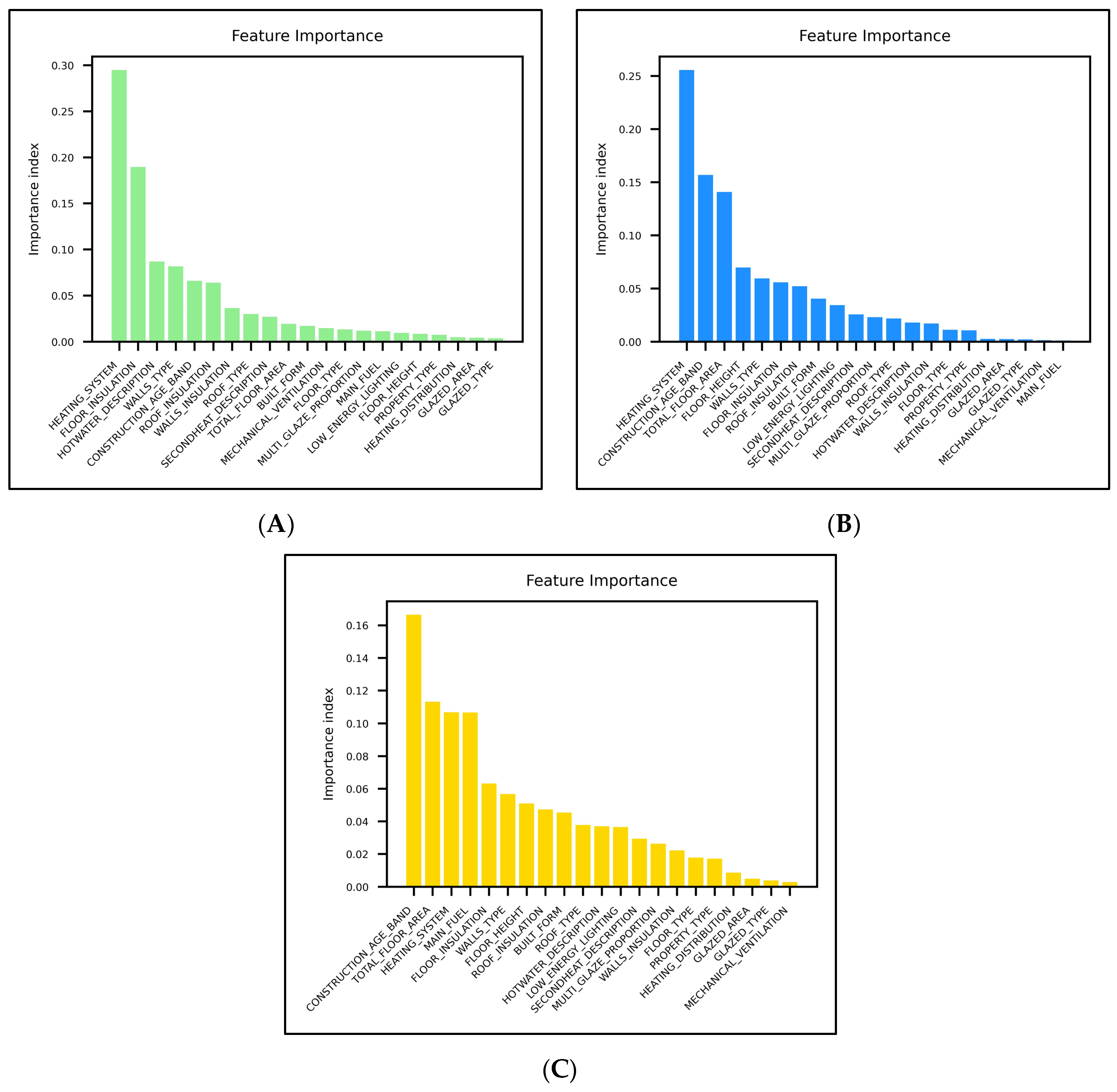
Considering the complexity of the objective function in this research, relying only on ML evaluation metrics may not provide a comprehensive understanding of the models’ performance. Therefore, the feature importance analysis for ensemble learning models, which highlights the relative significance of different feature in predicting building energy performance, is presented in Figure 6.

In this regard, the conducted analysis aligns with the fact that almost 63 percent of energy consumption in UK homes is related to space heating [5], in which both RF and XGB models highlight the “heating system” as the most important feature in predicting building energy performance, with relative importance scores of 0.26 and 0.29, respectively. Although the ET model also identifies “heating system” as the third most important feature, its relative score of 0.11 suggests a lower impact for this feature compared to the other models.

In the XGB model, other top important features are related to the building envelope (floor insulation, external wall type, and roof insulation) and have a direct impact on space heating. Moreover, “hot water system type”, which has the third ranking in the XGB model feature importance score, is another major energy consumer in UK homes, accounting for 17% of total energy demand [5]. These consistencies across all the models, particularly the XGB model, emphasize the accuracy of the developed model in terms of prioritizing critical features for building energy performance prediction.

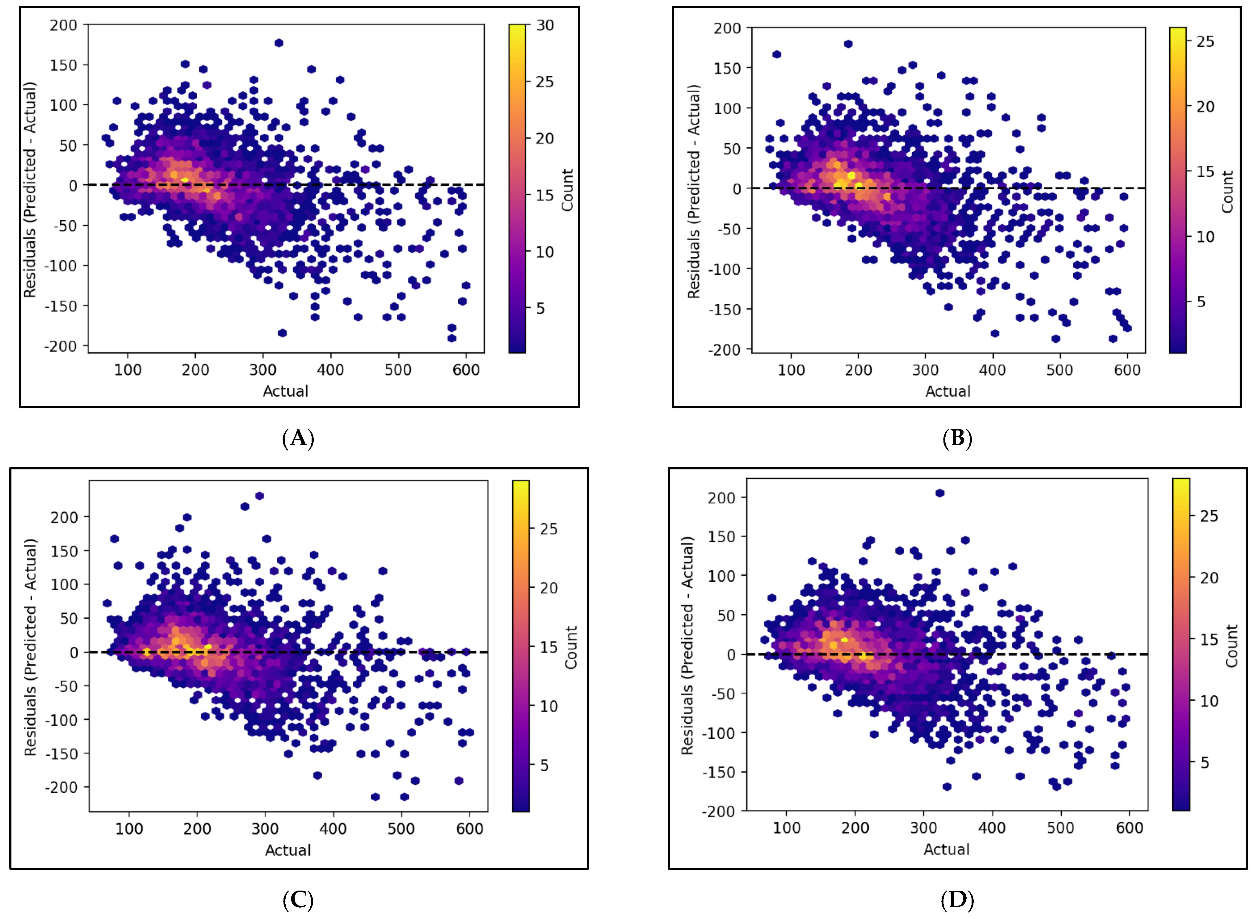
In order to get more insight about models’ predictive performance, Figure 7 displays the difference between the predicted and actual values of buildings’ annual energy consumption (Kwh/m²) for 2800 test cases. This figure reveals that concentration of residuals (actual–predicted) occurs around the central line “y = 0”, especially between lines “X = 100” and “X = 250”; which indicates higher accuracy of the models for case studies with actual annual energy consumption from 100 to 250 Kwh/m². Moreover, in this area, the plot appears to be relatively symmetric with a slight positive bias and some outliers (especially in ensemble models), suggesting potential areas for model refinement.

Lighter-density data points below the central line “y = 0” can be observed in the right side of the “X = 400” line, which indicates the negative bias of the models for these test case studies. All in all, based on the overall distribution of residuals, the ANN-MLP model appears to perform more robustly, with a smaller number of outliers, more symmetric, and concentration around the central line.

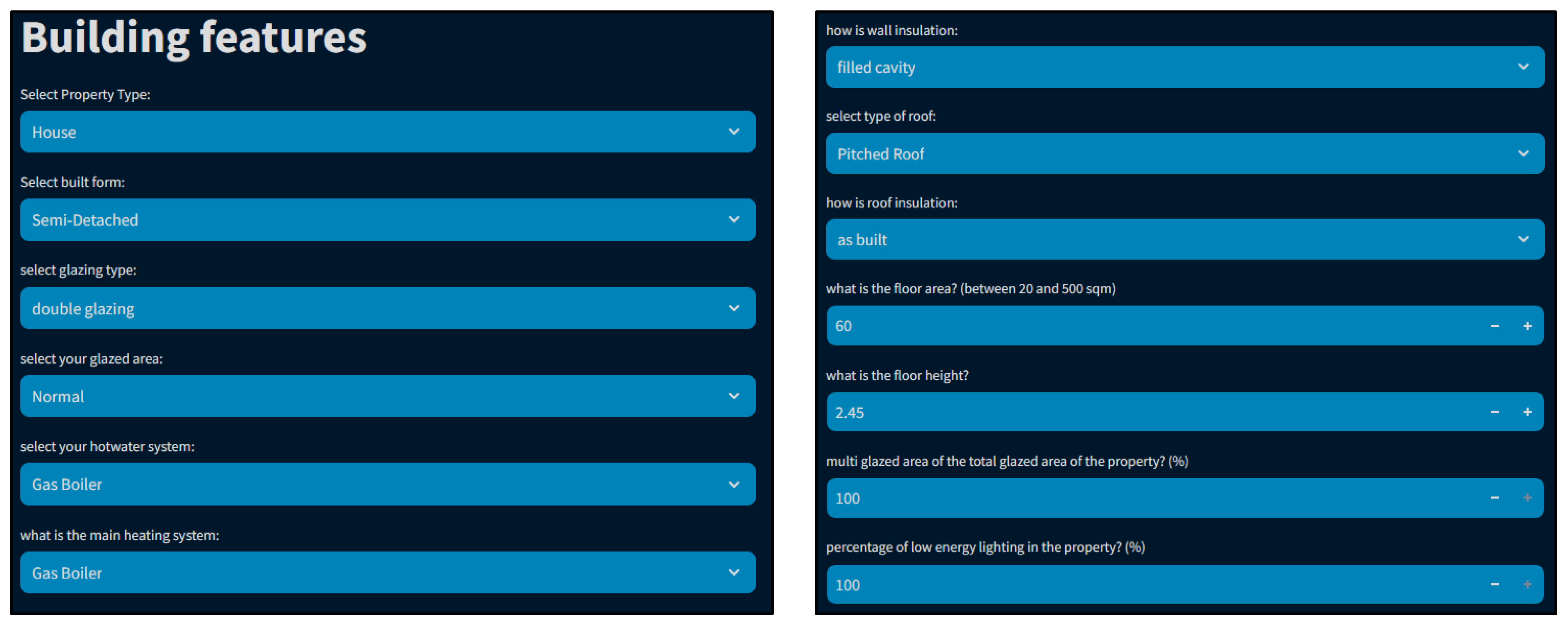
Furthermore, to investigate the performance of the developed models and ensure their conceptual functionality, a user interface was designed using the “Streamlit” framework. Figure 8 illustrates a capture of this interface, which enables users to input building features for a specific case study and observe the models’ prediction.

Through this interface, various characteristics can be modified, such as adding insulation to external walls or changing the heating system. By observing the response of each model, it can be evaluated whether the predictions align with the expected outcomes. For instance, when insulation is added, it is expected that annual energy consumption will decrease. Through this interactive analysis, the aim is to validate the models’ predictive accuracy and verify their ability to capture real-world changes in building characteristics.

In this context, a case study characterized by the features outlined in

Table 3. Case study building characteristics.

Property type:	Flat	Construction year:	1976–1982	Glazing type:	Double glazed
Built form:	Enclosed mid-terrace	Floor type and insulation:	Suspended, as-built	Roof type and insulation:	Another dwelling above
Hot water system:	Gas boiler	Heating system:	Gas boiler	Ventilation system:	Natural
External wall and insulation:	Cavity wall, as-built	Floor area:	60	Low-energy lighting (%):	100

was initially considered, representing the base case scenario. Subsequently, various retrofit strategies detailed in

Table 4. Effect of selected retrofit on case study’s energy performance.

Annual Energy Consumption Based on Model Prediction (Kwh/m2)				Possible Retrofits
XGB	RF	ET	ANN-MLP
176	190	191	181	Base case scenario
181	191	193	167	Changing windows to triple glazing
181	191	193	200	Single-glazed windows
284	192	243	169	Utilizing air source heat pump for hot water and heating system
217	190	197	188	Utilizing mechanical ventilation (supply + extract)
185	192	195	214	50% low-energy lighting
157	177	176	152	Adding internal insulation
156	180	186	140	Adding external insulation
188	177	176	186	Filling cavities and adding insulation

were examined to assess their potential impact on the case study’s energy performance.

It can be observed that adding insulation leads to a reduction in energy consumption across all the models, ranging from 20% in the ANN-MLP model to 4% in the ET model. This aligns with expectations as improved thermal insulation reduces heat loss and enhances energy efficiency. However, the amount of reduced energy consumption is more acceptable and realistic in the XGBoost and ANN-MLP models, which highlights their accuracy in this particular retrofit. On the other hand, filling cavity walls, which is another practice for energy efficiency in homes, does not result in an energy consumption reduction in the XGB and ANN-MLP models, which suggests an area for potential improvements in the models.

When utilizing an air source heat pump, only the ANN-MLP model predicts a reduction in energy consumption (around 7%), while a significant increase is recorded across all the other models. This may indicate a lack of accuracy among the ensemble learning models in this specific retrofit scenario. Overall, based on analysed data for this case study, it can be interpreted that the ANN-MLP model shows more reliability when dealing with potential retrofit interventions.

4. Discussion

The present study aimed to incorporate ML models along with SAP guidelines and the EPC dataset in the UK to design an AI tool which predicts annual primary energy consumption in residential buildings. The obtained results indicated that the model built on ANN-MLP showed the best performance in terms of both statistical metrics and predicting dynamic changes in building features. However, the validation results showed lower accuracy compared to the studies conducted by Seyedzadeh et al. [6] and Shao et al. [7]. This disparity could be justified considering that they utilized either a more detailed dataset for limited case studies or implemented on-site measurements.

Further comparisons with the works of Araujo et al. [9] and Razak et al. [4], who developed models based on residential buildings’ EPC certificate datasets in different countries with varying feature engineering approaches, revealed comparable levels of accuracy in terms of statistical metrics (R² value of around 0.8). However, it is important to note that the dynamic response of their models to building retrofits was not explicitly presented in their studies. This underscores the contribution of this research in evaluating the adaptability of AI tools to predict energy consumption changes resulting from building retrofits.

The analysis of feature importance in this study aligns with the findings of Razak et al. [3], particularly regarding the significance of building envelope-related features, such as wall type and floor insulation, which are among the top five factors influencing buildings’ energy consumption. On the other hand, while the heating system emerges as the most significant feature in this study and measured data [5], it is not among the top features affecting the predictive performance of the models developed by Razak et al. [3].

Moreover, the literature lacks detailed analyses of models’ predictive performance under specific conditions. Contrary to our results, which demonstrate minimal errors within the range of 150 to 250 kWh/m² of building energy consumption (as depicted in Figure 7), prior studies have not specified the conditions under which their models exhibit optimal performance. This gap highlights the need for more comprehensive investigations to better understand how contextual factors affect model performance and improve the reliability of energy consumption forecasts.

Moving forward, exploring the integration of additional factors such as control systems and occupant behaviour into predictive models could lead to more comprehensive and precise energy consumption forecasts.

5. Conclusions

In this paper, four machine learning models including XGBoost, random forest, extra trees, and an artificial neural network were developed based on the EPC database for residential buildings and standard assessment procedure (SAP) guidelines in the UK. Additionally, an interface was designed that enables user to analyse the effect of different retrofit strategies on a building’s energy performance. The results of this study indicate that the ANN-MLP model outperforms other machine learning models with a coefficient of determination (R²) of 0.82 and a mean percentage error of 11.9 percent. Across all the models, the heating system is the most influential feature in predicting building energy performance, followed by building envelope features such as wall type and insulation.

Furthermore, the obtained results suggest higher accuracy of the models in case studies with actual annual energy consumption ranging from 100 to 250 kWh/m², while some outliers have been observed in predicting case studies with annual energy consumption exceeding 400 kWh/m². Despite these challenges, these developed AI models offer a potential alternative or support to physics-based models in facilitating the retrofitting process of buildings. Utilizing the various datasets available, these models can contribute significantly to improving energy efficiency in residential buildings and ultimately help in achieving energy efficiency targets.