Inventory, Dynamic Evolution, and Scenario Projections of Agricultural Carbon Emissions in Shandong Province, China

Abstract

The reduction in agricultural carbon emissions (ACEs) in Shandong Province is essential to China’s carbon peak and carbon neutrality objectives. In this regard, we constructed an ACE inventory for Shandong Province at a resolution of 1 km × 1 km, integrating the emission factor method with geographic information system (GIS) technology. Building upon this, we explored the dynamic evolution patterns of ACEs using kernel density estimation and conditional probability density estimation. Additionally, long short-term memory networks were trained to predict ACEs under various scenarios. The results showed that: (1) ACEs in Shandong Province exhibited two stages of change, i.e., “rise and decline”. Notably, 64.39% of emissions originated from the planting industry. The distribution of emissions was closely correlated with regional agricultural production modes. Specifically, CO₂ emissions were predominantly distributed in crop cultivation areas, while CH₄ and N₂O emissions were primarily distributed in livestock breeding areas. The uncertainty of the emission inventory ranged from −12.04% to 10.74%, mainly caused by emission factors. (2) The ACE intensity of various cities in Shandong Province is decreasing, indicating a decoupling between ACEs and agricultural economic growth. Furthermore, the emission disparities among different cities are diminishing, although significant spatial non-equilibrium still persists. (3) From 2022 to 2030, the ACEs in Shandong Province will show a continuous downward trend. By 2030, the projected values under the baseline scenario, low-carbon scenario I, and low-carbon scenario II will be 6301.74 × 10⁴ tons, 5980.67 × 10⁴ tons, and 5850.56 × 10⁴ tons. The low-carbon scenario reveals greater potential for ACE reduction while achieving efficient rural economic development and urbanization simultaneously. This study not only advances the methodology of the ACE inventory but also provides quantitative references and scientific bases for promoting low-carbon, efficient, and sustainable regional agriculture.

1. Introduction

Greenhouse gas (GHG) emissions have become a major driver of climate change, leading to global warming and an increase in extreme weather events. Countries around the world have recognized the urgency of the situation and have reached a global consensus on reducing GHG emissions. As a leader and pioneer in international low-carbon actions, China announced in 2020 its aim to peak CO₂ emissions before 2030 and strive to achieve carbon neutrality by 2060. Agricultural production is a significant contributor to anthropogenic GHG emissions [1], accounting for about 14% of the global total [2] and growing at an annual average rate of 1.1% [3]. Both China and the United States are agricultural powerhouses. However, while agricultural carbon emissions (ACEs) in the United States account for only 6.3% of its total emissions [4], China’s ACEs reach as high as 17% [5]. Therefore, ACE reduction is crucial for China to achieve its “dual carbon” goals. Additionally, there are regional differences in agricultural location and resource endowments across China, making it necessary to conduct in-depth research on ACEs in specific regions.

Research on ACEs began with the identification of emission sources, initially focusing on inputs such as fertilizers, pesticides, and irrigation in agriculture [6,7,8,9,10]. Subsequently, researchers delved into carbon sources related to rice cultivation [11,12], agricultural land [13,14], and straw burning [15,16], as well as animal enteric fermentation and manure management [17,18,19]. Scholars have inherited and expanded on related research findings, resulting in a more diversified trend in ACE sources, which now largely cover both crop cultivation and livestock farming, the two main sectors of agricultural production. Unified standards for calculating ACEs have not yet been established. The main measurement techniques include the emission factor method [20,21,22,23], life cycle assessment [24], and the modeling method [25]. The modeling method requires complex data and calculations, while life cycle assessment entails higher costs. Both methods have limitations in estimating emissions over long periods and at large scales. In contrast, the emission factor method possesses both macroscopic and microscopic characteristics, is highly adaptable, and has mature formulas, activity levels, and emission factor databases. It can relatively accurately reflect the emission status of sources and has been widely adopted internationally [26], including in China’s “Guidelines for the Compilation of Provincial Greenhouse Gas Inventories”. After compiling ACE inventories, scholars further studied the characteristics of ACEs and their future carbon emission reduction potential. Assessment of ACE characteristics is typically based on efficiency [27,28,29] or intensity [30,31,32,33], analyzing their spatiotemporal distribution using techniques such as kernel density estimation, Markov chain, standard deviation ellipse, and Gini coefficient. Regarding predictions of future ACE reduction potential, research approaches can be broadly categorized into two types. The first involves using methods such as the Kaya constant equation, the logarithmic mean Divisia index, or the stochastic impacts by regression on population, affluence, and technology (STIRPAT) model to determine ACE influencing factors and combining them with scenario analysis to predict ACEs [34,35,36]. The second type utilizes system modeling methods such as grey prediction or autoregressive integrated moving averages to directly forecast ACEs based on historical data [37,38]. Currently, the STIRPAT model combined with scenario analysis is the mainstream forecasting method [39]. This approach can incorporate regional policy planning and agricultural conditions, exploring scenarios that maximize future ACE reduction potential and promote sustainable agricultural development.

While current research on ACEs has yielded significant contributions, several challenges persist: (1) carbon sources such as crops, agricultural land, and straw burning are often overlooked in ACE measurements, leading to underestimated emissions. (2) ACE inventories are typically compiled based on administrative divisions as spatial statistical units, which do not accurately identify their characteristics. Moreover, there is a lack of quantitative assessment of the reliability of ACE inventories, i.e., uncertainty analysis. (3) There is insufficient understanding of the continuity and mobility of ACE distribution, hindering research on its dynamic evolutionary patterns. (4) The absence of robust learning and testing processes in ACE prediction may lead to drawbacks example overfitting, vague nonlinear relationships, and low generalization ability.

Shandong Province is a crucial agricultural production center in China, with its gross agricultural output value, agricultural value-added, and total agricultural import and export value ranking first nationwide. Therefore, we selected Shandong Province as the research subject. To overcome the limitations of previous studies, we developed a more comprehensive ACE measurement framework, encompassing five crucial domains: soil utilization, crop planting, straw burning, enteric fermentation, and manure management. The ACE inventory, with a spatial resolution of 1 km × 1 km, was generated by integrating the emission factor method and geographic information system (GIS) technology, and its uncertainty was quantitatively analyzed through Monte Carlo simulation. Subsequently, kernel density and conditional probability density estimation techniques were employed to examine the dynamic evolution patterns and spatial heterogeneity of ACEs. Finally, we trained a long short-term memory (LSTM) network to predict ACEs in Shandong Province under various scenarios.

2. Materials and Methods

2.1. Study Area

Shandong Province is located on the east coast of China, spanning from 34°22′ N to 38°24′ N and from 114°47′ E to 122°42′ E. It shares its borders with Hebei, Henan, Anhui, and Jiangsu provinces, from north to south. The province comprises 16 prefecture-level cities and covers a total area of 15.58 × 10⁴ km² (Figure 1). The region experiences a temperate monsoon climate, characterized by an average annual light duration of 2290–2890 h, a temperature range of 11–14 °C, and rainfall between 550 and 950 mm. With abundant light, heat, and water resources, Shandong is highly conducive to the growth of various crops and livestock. In 2022, the planting industry in the province generated a total output value of CNY 620.65 billion, while animal husbandry contributed to a total output value of CNY 300.35 billion. The main crops cultivated in the province include wheat, maize, sweet potatoes, soybeans, rice, and peanuts. Livestock farming primarily involves cattle, pigs, sheep, poultry, and rabbits.

2.2. Data Sources

The calculation of Shandong ACEs spanned the years 2000–2021, incorporating data from multiple sources including statistical data, emission factor data, and geospatial data. Specifically, activity level data for ACE sources were obtained from the Shandong Provincial Statistical Yearbooks (2001–2022). Emission factor data for ACE sources were obtained from reputable references such as the Intergovernmental Panel on Climate Change (IPCC), the Guidelines for the Compilation of Provincial Greenhouse Gas Inventories, and relevant literature. Administrative boundary data were acquired from the Resources and Environment Data Centre of the Chinese Academy of Sciences (https://www.resdc.cn/DOI/DOI.aspx?DOIid=121, accessed on 2 July 2023). Additionally, land cover data with a spatial resolution of 30 m were obtained from the Zenodo platform (https://zenodo.org/record/5816591#.ZCJIR8pBz1_, accessed on 6 April 2023).

2.3. Measuring Method of ACEs

We employed the emission factor method, which is recommended by the IPCC, to quantify ACEs. The total ACEs are calculated by summing up emissions from various carbon sources, as expressed below:

$$E=E_{\mathrm{soil}}+E_{\mathrm{crop}}+E_{\mathrm{straw}}+E_{\mathrm{enteric}}+E_{\mathrm{manure}}$$

(1)

where E represents the total ACEs, E_soil denotes the carbon emissions from soil utilization, E_crop signifies carbon emissions from crop planting, E_straw indicates carbon emissions from straw burning, E_enteric refers to carbon emissions from enteric fermentation, and E_manure represents carbon emissions from manure management. CH₄ and N₂O are expressed in CO₂ equivalents (CO₂-eq) based on the global warming potential, with 1 kg of CH₄ being equivalent to 28 kg of CO₂ and 1 kg of N₂O being equivalent to 265 kg of CO₂ [40].

The agricultural carbon emission intensity (ACEI) is defined as the carbon emissions per unit of growth in agricultural GDP [41], expressed as:

$$ACEI=E/AGDP$$

(2)

where AGDP is the gross value of agricultural production.

2.3.1. Carbon Emissions from Planting

(1)

Soil Utilization

Carbon emissions from soil utilization consist of two aspects, CO₂ emissions from agricultural inputs, represented by E_material, and N₂O emissions from agricultural land, represented by E_land:

$$E_{\mathrm{soil}}=E_{\mathrm{material}}+E_{\mathrm{land}}\times 265$$

(3)

CO₂ emissions from agricultural inputs relate to fertilizers, agricultural films, agricultural diesel, pesticides, plowing, and irrigation:

$$E_{\mathrm{material}}={\displaystyle \sum _{s=1}^t{E}_{\mathrm{material},s}}={\displaystyle \sum _{s=1}^t{A}_{\mathrm{material},s}}\times E{F}_{mc,s}\times 44/12$$

(4)

where E_material,s, A_material,s, and EF_mc,s are the CO₂ emissions, activity levels, and emission factors of the agricultural land material s, respectively. The emission factors are given in

Table 1. Carbon emission sources and emission factors of agricultural inputs.

Emission Source		Emission Factor	References
Chemical fertilizer	Nitrogen fertilizer	0.4173 kg(C)∙kg−1	Fan [1]
	Phosphate fertilizer	0.4445 kg(C)∙kg−1
	Potash fertilizer	0.1773 kg(C)∙kg−1
	Compound fertilizer	0.4827 kg(C)∙kg−1
Agricultural film		5.18 kg(C)∙kg−1	Tian [42]
Agricultural diesel oil		0.5927 kg(C)∙kg−1	IPCC [2]
Pesticide		4.9341 kg(C)∙kg−1	Zhi and Gao [43]
Plowing		312.6 kg(C)∙hm−2	Wu [44]
Irrigation		19.8575 kg(C)∙kg−1	Wu [32]

Note: CO₂ emission factor = carbon emission factor × 44/12.

.

N₂O emissions from agricultural land are divided into direct and indirect emissions:

$$E_{\mathrm{land}}=E_{\mathrm{direct}}+E_{\mathrm{indirect}}$$

(5)

where E_direct and E_indirect are direct and indirect N₂O emissions from agricultural land, respectively.

Direct emissions arise from in-season nitrogen inputs to agricultural land, including fertilizer, manure, and straw. Due to the difficulty of obtaining data on manure application, only fertilizer and straw were considered.

$$E_{\mathrm{direct}}=(N_{nf}+N_{sr})\times E{F}_{dt}$$

(6)

$$N_{sr}={\displaystyle \sum _{j=1}^q{N}_{sr,j}}={\displaystyle \sum _{j=1}^q\left(\left(\frac{Y_j}{M_j}-Y_j\right)\times P_j\times R\times D_j+\frac{Y_j}{M_j}\times P_j\times G_j\times D_j\right)}$$

(7)

where N_nf and N_sr represent nitrogen inputs from nitrogen fertilizers and straw returns, respectively. EF_dt is the direct emission factor of N₂O from agricultural land (0.0057 kg(N₂O)∙kg⁻¹) [45]. For crop j, N_sr,j, Y_j, M_j, P_j, R, D_j, and G_j represent nitrogen inputs, economic yields, economic coefficients, the proportion of nitrogen in straw, the straw return rate (56%) [22], the dry weight ratio, and the root-to-crown ratio, respectively. The measured parameters are listed in

Table 2. Parameters for measuring nitrogen in straw returned to the field by crop [45].

Crop	Dry Weight Ratio	Proportion of Nitrogen in Straw	Economic Coefficient	Root-to-Crown Ratio
Rice	0.855	0.00753	0.489	0.125
Wheat	0.87	0.00516	0.434	0.166
Maize	0.86	0.0058	0.438	0.17
Beans	0.82	0.022	0.385	0.13
Tubers	0.45	0.011	0.667	0.05
Peanuts	0.9	0.0182	0.556	0.2
Rapeseed	0.82	0.00548	0.271	0.15
Vegetables	0.15	0.008	0.83	0.25

.

Indirect emissions originate from atmospheric nitrogen deposition, as well as nitrogen loss through leaching and runoff:

$$E_{\mathrm{indirect}}=E_{nd}+E_{lr}=(N_{nf}+N_{sr})\times V\times E{F}_{nd}+(N_{nf}+N_{sr})\times L\times E{F}_{lr}$$

(8)

where E_nd represents N₂O emissions from atmospheric nitrogen deposition, E_lr is N₂O emissions from leaching and runoff. V, EF_nd, L, and EF_lr denote the volatilization rate (10%), the atmospheric nitrogen deposition emission factor (0.01 kg(N₂O) kg⁻¹), the loss rate (20%), and the leaching and runoff emission factor (0.0075 kg(N₂O)∙kg⁻¹), respectively [45].

(2)

Crop Planting

Carbon emissions from crop cultivation include CH₄ emissions from rice fields and N₂O emissions from major crops:

$$E_{\mathrm{crop}}=E_{\mathrm{rice}}\times 28+{\displaystyle \sum _{j=1}^q{E}_{\mathrm{crop},j}}\times 265=A_{\mathrm{rice}}\times E{F}_{\mathrm{rice}}\times 28+{\displaystyle \sum _{j=1}^q{A}_{\mathrm{crop},j}}\times E{F}_{cc,j}\times 265$$

(9)

where E_rice, A_rice, and EF_rice represent CH₄ emissions, sown area, and CH₄ emission factors for rice fields, respectively. For crop j, E_crop,j, A_crop,j, and EF_cc,j denote N₂O emissions, sown area, and N₂O emission factors, respectively. The emission factors are given in

Table 3. Carbon emission sources and emission factors of crop cultivation.

Emission Source	Emission Factor	References
Rice	215.5 kg(CH4)∙hm−2	PRC National Development and Reform Commission [45]
	0.24 kg(N2O)∙hm−2	Min and Hu [46]
Wheat	1.75 kg(N2O)∙hm−2
Maize	2.532 kg(N2O)∙hm−2
Beans	2.29 kg(N2O)∙hm−2
Tubers	0.95 kg(N2O)∙hm−2
Peanuts
Rapeseed
Vegetables	4.944 kg(N2O)∙hm−2
Cotton	0.4804 kg(N2O)∙hm−2	Liu and Liu [47]
Melons	4.21 kg(N2O)∙hm−2	Xie And Liu [48]

.

(3)

Straw burning

Carbon emissions from straw burning are calculated by:

$$E\mathrm{straw}={\displaystyle \sum _{j=1}^q\left(E_{sh,j}\times 28+E_{sc,j}\right)}={\displaystyle \sum _{j=1}^q\left[\left(Y_j\times S_j\times B_j\times X_j\right)\times \left(E{F}_{sh,j}\times 28+E{F}_{sc,j}\right)\right]}$$

(10)

where S_j represents the straw-to-grain ratio of crop j; E_sh,j, E_sc,j, B_j, X_j, EF_sh,j, and EF_sc,j denote the CH₄ emissions, CO₂ emissions, burning ratio, burning efficiency, CH₄ and CO₂ emission factors for straw burning of crop j, respectively. The measured parameters are listed in

Table 4. Parameters for measuring the straw burning of major crops [22].

Emission Source	Straw-to-Grain Ratio	Burning Ratio	Burning Efficiency	Emission Factor (kg∙kg−1)
				CH4	CO2
Rice	0.93	0.097	0.93	0.0032	1.46
Wheat	1.34	0.197	0.93	0.0034	1.46
Maize	1.73	0.234	0.92	0.0044	1.35

.

2.3.2. Carbon Emissions from Animal Husbandry

(1)

Enteric Fermentation

Microorganisms in the digestive tract produce CH₄ emissions through fermentation during the normal metabolic process of livestock:

$$E_{\mathrm{enteric}}={\displaystyle \sum _{k=1}^l{E}_{\mathrm{enteric},k}}\times 28={\displaystyle \sum _{k=1}^l{A}_{\mathrm{livestock},k}}\times E{F}_{eh,k}\times 28$$

(11)

where E_enteric,k, A_livestock,k, and EF_eh,k represent the CH₄ emissions from livestock enteric fermentation, year-end stock, and emission factors, respectively.

(2)

Manure Management

Livestock manure emits CH₄ and N₂O during storage and handling before application to soil:

$$E_{\mathrm{manure}}={\displaystyle \sum _{k=1}^l{E}_{mh,k}}\times 28+{\displaystyle \sum _{k=1}^l{E}_{mn,k}}\times 265={\displaystyle \sum _{k=1}^l{A}_{\mathrm{livestock},k}}\times \left(E{F}_{mh,k}\times 28+E{F}_{mn,k}\times 265\right)$$

(12)

where E_mh,k, E_mn,k, EF_mh,k, and EF_mn,k represent the CH₄ emissions, N₂O emissions, CH₄ and N₂O emission factors for livestock manure management, respectively. The emission factors are provided in

Table 5. Carbon emission sources and emission factors of animal husbandry (kg∙head⁻¹∙year⁻¹).

Emission Source	Enteric Fermentation	Manure Management		References
	CH4	CH4	N2O
Cattle	80.125	5.73	1.262	PRC National Development and Reform Commission [45]
Pig	1	5.08	0.175
Sheep	8.2333	0.27	0.113
Poultry	–	0.02	0.007
Rabbit	0.254	0.08	0.02	Hu and Wang [49]

Note: There are variations in carbon emission factors for different rearing sizes and types of cattle and sheep. We utilized the average value in our calculation.

.

2.4. Kernel Density Analysis

Kernel density analysis, a significant non-parametric estimation method, demonstrates strong robustness and is not dependent on a particular model. Consequently, it has become a widely employed technique for investigating non-uniform distribution problems. Kernel density analysis can generate continuous and smooth density curves by estimating the probability density of random variables. This approach accurately illustrates the distribution pattern of random variables and thus aids in elucidating the dynamic evolution trend of ACE.

2.4.1. Kernel Density Estimation

Kernel density estimation was proposed by Mood [50] and Silverman [51]. Let the density function of a set of continuous random variables X be denoted by f(x) and the probability density of the point x is given by:

$$f(x)=\frac{1}{nh}{\displaystyle \sum _{i=1}^{n}K(\frac{X_i-\overline{x}}{h})}$$

(13)

$$K(x)=\frac{1}{\sqrt{2\pi }}\exp (-\frac{x^2}{2})$$

(14)

where n, h, X_i, and $\overline{x}$ represent the number of observations, bandwidth, independently and identically distributed observations, and mean, respectively. K(·) denotes the Gaussian kernel function.

2.4.2. Conditional Probability Density Estimation

The conditional probability density estimation proposed by Hyndman et al. [52] can reflect the continuity and mobility of the ACE distribution more comprehensively and intuitively than kernel density estimation and the Markov chain. Its expression is:

$$g(y|x)=\frac{f(x,y)}{f(x)}$$

(15)

$$f(x,y)=\frac{1}{n{h}_x{h}_y}{\displaystyle \sum _{i=1}^{n}K(\frac{X_i-\overline{x}}{h_x})}K(\frac{Y_i-\overline{y}}{h_y})$$

(16)

where $g(y|x)$ denotes the conditional probability density of y under the given x condition. f(x,y) represents the joint density function of x and y.

2.5. LSTM

LSTM is an advancement and refinement of the recurrent neural network (RNN) architecture. It was originally proposed by Hochreiter and Schmidhuber [53] and further improved and popularized by Graves [54]. LSTM addresses the problem of vanishing gradients in traditional RNNs through the introduction of memory cells and gating mechanisms. This enables LSTM to effectively learn dependencies in time-series data with strong temporal order and non-linearity, thereby making it suitable for predicting ACE.

LSTM consists of four main components: an input gate, a forget gate, an output gate, and a memory cell. In addition, three control gates are connected to the multiplication unit to control the input, memory cell, and output of the LSTM unit. The memory cell has a forgetting mechanism determined by its current state, the input of the forget gate x_t, and the previous intermediate output h_t−1. The memory cell also has a retention vector that combines the result of the input gate’s transformation (x_t transformed by the tanh and sigmoid functions) with the updated memory cell state. The intermediate output h_t is determined based on the updated memory cell state and the output gate. The primary calculation equations for LSTM are as follows:

$$i_t=\sigma \left(W_{ix}{x}_t+W_{ih}{h}_{t-1}+b_i\right)$$

(17)

$$o_t=\sigma \left(W_{ox}{x}_t+W_{oh}{h}_{t-1}+b_o\right)$$

(18)

$$f_t=\sigma \left(W_{fx}{x}_t+W_{fh}{h}_{t-1}+b_f\right)$$

(19)

$$g_t=\varphi \left(W_{gx}{x}_t+W_{gh}{h}_{t-1}+b_g\right)$$

(20)

$$S_t=g_t\odot i_t+S_{t-1}\odot f_t$$

(21)

$$h_t=\varphi \left(S_t\right)\odot o_t$$

(22)

where σ and ϕ denote the sigmoid and tanh functions, respectively. i_t, o_t, f_t, h_t, g_t, and S_t denote the input gate, the output gate, the forget gate, the intermediate output node, the intermediate input node, and the state unit, respectively. W_ix, W_ih, W_ox, W_oh, W_fx, W_fh, W_gx, and W_gh denote the weights of the inputs x_t and the intermediate output h_t−1 matrix. $\odot$ denotes the Hadamard product. b_i, b_o, b_f, and b_g denote the bias of each corresponding gate.

3. Results

3.1. ACE Inventory

Table 6. ACE inventory in Shandong Province from 2000 to 2021 (10⁴ tons).

Years	Planting Industry						Animal Husbandry			Total Emissions
	Soil Utilization		Crop Planting		Straw Burning		Enteric Fermentation	Manure Management
	N2O	CO2	CH4	N2O	CH4	CO2	CH4	CH4	N2O
2000	491.62	2445.71	106.65	666.24	111.73	1420.60	2841.45	572.30	644.25	9300.55
2001	488.67	2527.32	96.14	656.92	111.32	1396.39	2870.14	592.82	662.01	9401.73
2002	466.15	2698.60	93.70	660.07	99.21	1249.36	2961.47	612.36	684.02	9524.94
2003	449.64	2724.59	63.29	644.70	97.91	1230.14	3119.03	644.10	718.58	9691.99
2004	460.57	2741.41	75.27	642.88	110.53	1374.40	3276.69	680.47	758.57	10120.78
2005	477.71	2825.96	72.49	676.23	130.38	1642.84	3108.18	667.32	726.12	10327.22
2006	490.21	2919.22	75.98	684.71	143.55	1811.56	2433.67	563.44	598.68	9721.01
2007	490.10	2922.40	77.76	677.80	148.15	1859.56	1919.76	500.78	489.61	9085.93
2008	443.97	2935.31	77.99	679.80	156.62	1968.13	2042.24	558.05	534.82	9396.93
2009	436.07	2856.22	78.42	693.06	172.34	2154.83	2103.63	604.43	568.65	9667.64
2010	432.10	2887.46	76.70	702.37	177.14	2213.25	2123.05	635.61	588.47	9836.15
2011	425.18	2873.85	75.06	707.08	183.60	2288.51	2146.15	669.11	609.76	9978.31
2012	424.44	2923.91	61.48	687.36	176.92	2200.33	2172.67	688.60	625.93	9961.63
2013	416.99	2901.54	65.79	674.48	162.98	2038.16	2138.74	698.73	620.81	9718.21
2014	410.36	2793.63	64.82	673.72	169.36	2113.79	2098.25	689.86	607.08	9620.85
2015	402.06	2824.74	60.19	669.82	166.82	2088.90	1911.87	656.66	573.64	9354.70
2016	389.44	2795.32	56.01	658.59	161.30	2021.90	1679.80	631.00	541.52	8934.88
2017	379.36	2722.88	65.93	698.69	180.16	2232.75	1390.65	550.43	473.11	8693.97
2018	360.58	2631.15	68.92	697.44	177.17	2197.88	1218.78	522.72	444.96	8319.59
2019	338.34	2497.42	69.97	693.67	176.81	2202.75	1170.55	472.77	447.20	8069.48
2020	328.35	2365.33	68.11	695.15	179.87	2237.82	964.79	517.43	420.68	7777.54
2021	308.72	2393.42	68.44	702.53	181.18	2259.01	1057.95	552.80	443.49	7967.54

presents the ACE inventory in Shandong Province from 2000 to 2021. Regarding the composition of agricultural GHGs, CO₂ dominates with a total contribution rate of 50.09%, followed by CH₄ and N₂O, which contribute 31.80% and 18.11%, respectively. There is an overall upward trend in CO₂ emissions (contribution rate), rising from 3866.30 × 10⁴ tons (41.57%) in 2000 to 4652.43 × 10⁴ tons (58.39%) in 2021. In contrast, CH₄ and N₂O emissions (contribution rate) show an overall decreasing trend, falling from 3632.14 × 10⁴ tons (39.05%) and 1802.11 × 10⁴ tons (19.38%) in 2000 to 1860.37 × 10⁴ tons (23.35%) and 1454.74 × 10⁴ tons (18.26%) in 2021, respectively.

Regarding the structure of the ACEs, the primary source is soil utilization with a total contribution of 34.00%. It is succeeded by enteric fermentation, straw burning, manure management, and crop planting with contributions of 22.86%, 22.29%, 12.75%, and 8.10% respectively. The emissions (contribution rate) of the planting industry show an overall increasing trend, rising from 5242.55 × 10⁴ tons (56.37%) in 2000 to 5913.29 × 10⁴ tons (74.22%) in 2021. Conversely, animal husbandry emissions (contribution rate) show an overall decreasing trend, decreasing from 4058.00 × 10⁴ tons (43.63%) in 2000 to 2054.24 × 10⁴ tons (25.78%) in 2021.

Overall, emissions in Shandong Province exhibit a pattern of initial increase followed by a subsequent decrease, with the average annual growth rate being −0.73%. Between 2000 and 2005, the total emissions experienced an upward trend, increasing from 9300.55 × 10⁴ tons to 10327.22 × 10⁴ tons, representing an increment of 11.04% and an average annual growth rate of 2.12%. However, from 2005 to 2021, the trend reversed, with a decline in total emissions. The total emissions reached 7967.54 × 10⁴ tons in 2021, a decrease of 22.85% from the peak in 2005 and an average annual decrease of 1.61%.

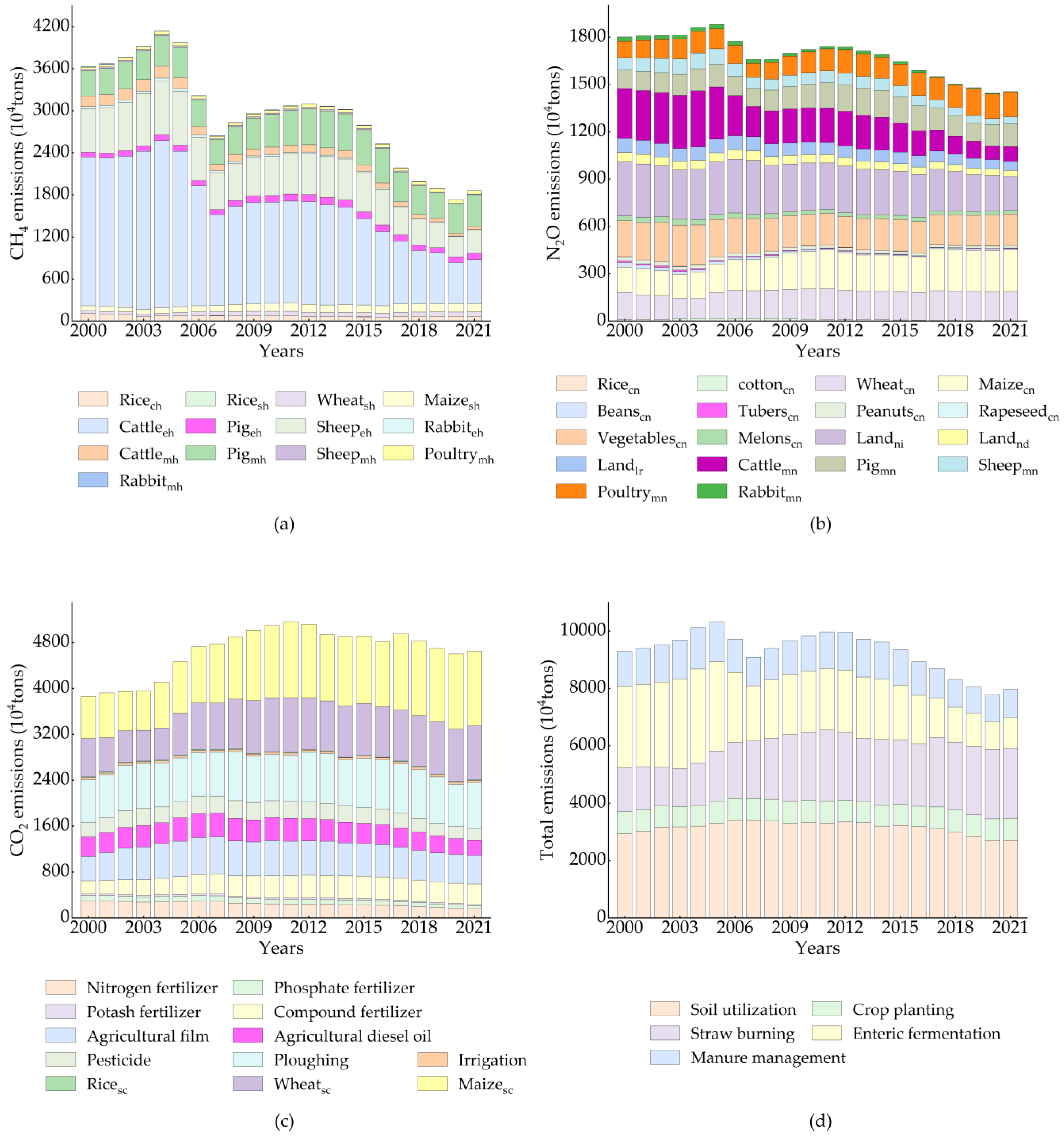
The emission structures of CH₄, N₂O, CO₂, and total emissions from agriculture in Shandong Province between 2000 and 2021 are depicted in Figure 2. Major sources of CH₄ emissions include enteric fermentation in cattle and sheep, as well as manure management in pigs. With Shandong Province undergoing industrial restructuring in animal husbandry, there has been a reduction in the number of large livestock requiring long feeding cycles and high farming costs. Consequently, CH₄ emissions from animal husbandry have decreased rapidly in recent years. N₂O emissions originate from various sources, including both the planting industry and animal husbandry. However, the reduction in emissions from animal husbandry has led to the planting industry becoming the primary source of N₂O emissions. The main source of CO₂ emissions is the plowing and burning of wheat and maize straw. In response to measures by the Chinese Ministry of Agriculture to reduce the use of chemical fertilizers and pesticides and to improve the efficiency of agricultural inputs, CO₂ emissions from agricultural inputs have been steadily decreasing. Nevertheless, due to the rise in crop productivity and inadequate comprehensive utilization of straw, straw burning has emerged as the foremost contributor to CO₂ emissions.

The total emissions trend indicates an annual rise in carbon emissions from straw burning, whereas carbon emissions from enteric fermentation and manure management have consistently decreased. Currently, the planting industry serves as the primary source of ACEs in all cities across the province.

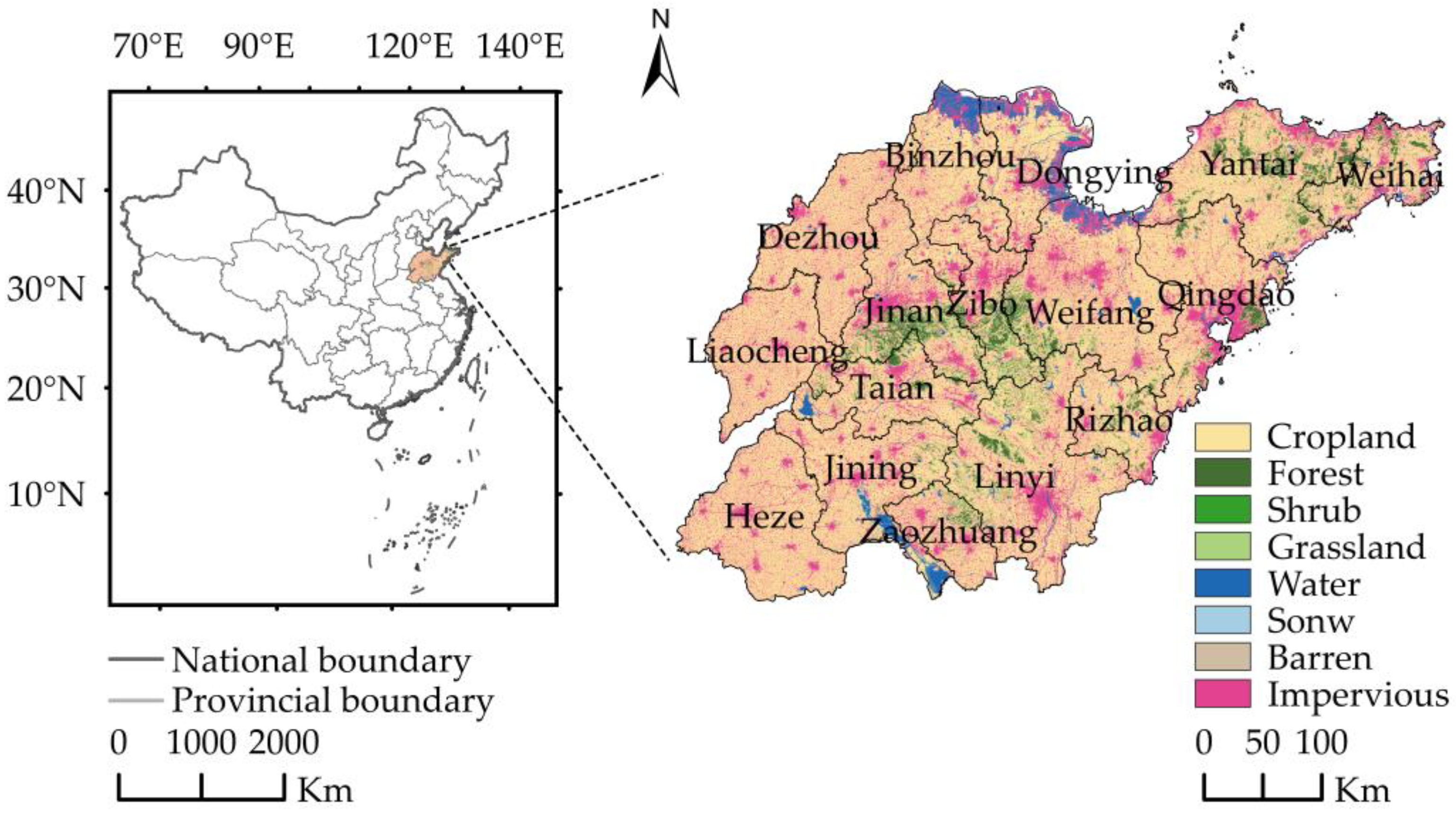
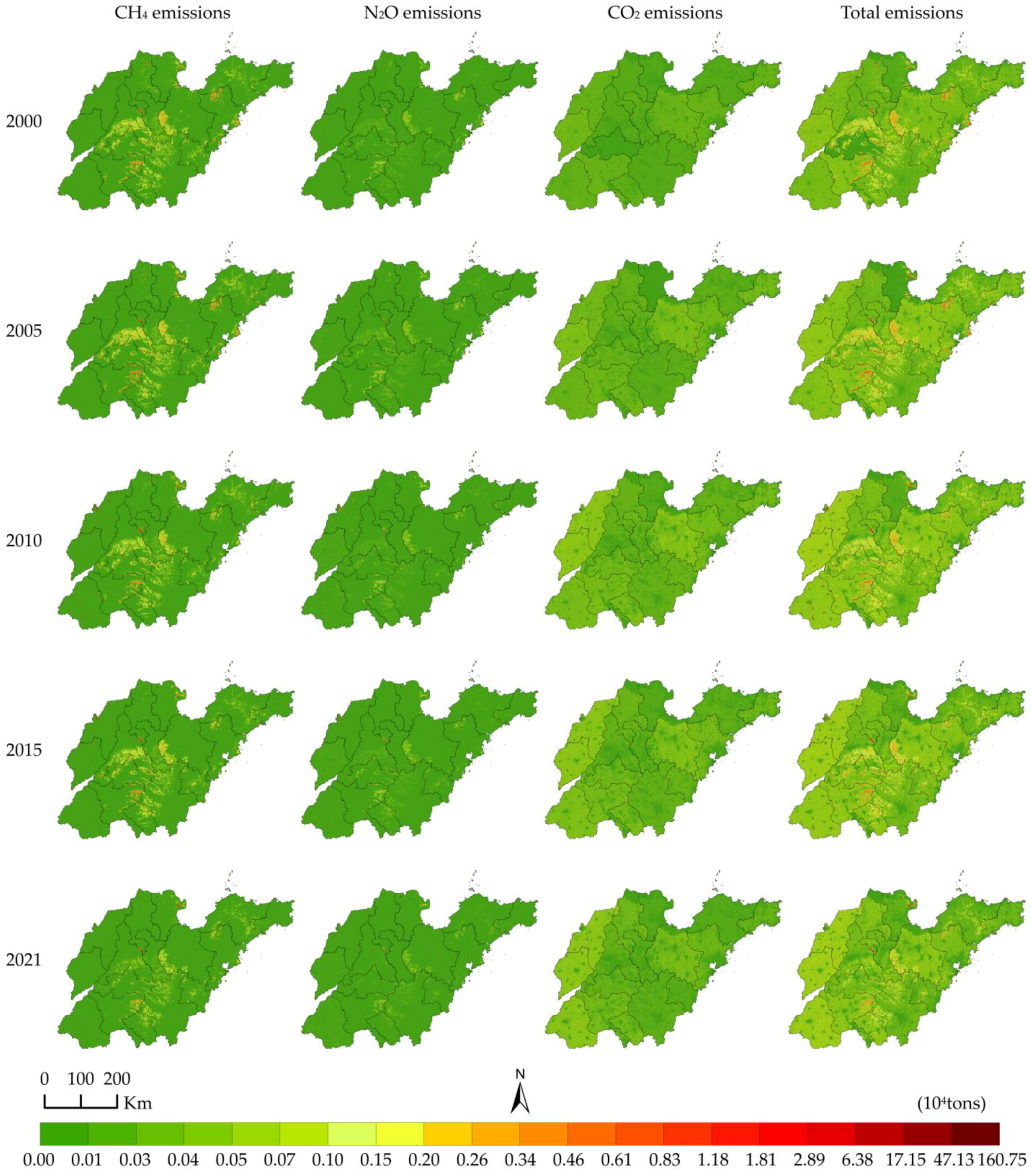
Spatial allocation of ACEs in Shandong Province was conducted using ArcGIS 10.8 software. The 30 m resolution cropland raster data were chosen to characterize the emissions from the planting industry. The GHG emissions per unit area of the emission sources within the planting industry in each city served as the spatial allocation factors. By connecting the gridded administrative division data (1 km × 1 km) with the cropland raster data, the corresponding GHG emissions within each grid were obtained. This involved multiplying each GHG’s spatial allocation factor with the cropland area within the grid. Similarly, 30 m resolution grassland raster data characterized emissions from animal husbandry, and emissions within the corresponding grid were calculated. Emissions of the same GHG from different sources were summed to derive the inventory for CH₄, N₂O, CO₂, and total emissions (Figure 3).

The spatial and temporal distribution of agricultural GHG emissions in Shandong Province is closely related to regional agricultural production methods. Specifically, CH₄ emissions are concentrated mainly in the mountainous and hilly areas of central, southern, and eastern Shandong Province, along with some areas of Binzhou and Dongying. These areas are suitable for grazing and constitute the main distribution areas for animal husbandry in Shandong Province, so the grids with higher emissions are mostly concentrated here. CH₄ emissions experienced a slight increase in some regions of Yantai, central and southern Shandong, between 2000 and 2005. However, from 2005 to 2021, the emission distribution shifted gradually towards central and southern Shandong. N₂O emissions are mainly concentrated in the mountainous and hilly areas of central and southern Shandong Province, as well as some areas of Yantai and Weifang. Between 2000 and 2021, N₂O emissions in Shandong Province decreased, and the main source of emissions shifted to the planting industry, so the emission distribution tends to spread to the southwest and northwest plains of Shandong Province which are suitable for the development of the planting industry. CO₂ emissions are more uniformly distributed compared to CH₄ and N₂O emissions. The emissions are mostly concentrated in the plains of southwest and northwest Shandong Province and part of Weifang. These regions contain extensive croplands where dryland crops predominate and have a large residual amount of straw leading to higher CO₂ emissions. From 2000 to 2021, CO₂ emissions increased in the southwest and northwest plains, as well as the eastern hilly areas of Shandong Province.

In general, ACEs tend to spread from the central and southern regions of Shandong Province to the southwest, northwest, and east regions as emissions from the planting industry increase and those from animal husbandry decrease in the province.

Monte Carlo stochastic simulation sampling was utilized to evaluate the uncertainty in the ACE inventory of Shandong Province. This technique enabled quantitative analysis of uncertainty and identification of the primary sources of uncertainty. The Oracle Crystal Ball add-in for Microsoft Excel 2013 software was employed for this purpose. The simulation made several assumptions about the input data. The activity levels of the emission sources were assumed to follow a normal distribution. The emission factors derived from the IPCC and the Guidelines for the Compilation of Provincial Greenhouse Gas Inventories were assumed to follow a uniform distribution, while the remaining emission factors were assumed to follow a normal distribution. ACEs were considered as the output and the relationship between the input variables (activity levels and emission factors) and the output was established. Random sampling was conducted using the Latin hypercube sampling scheme. Through 10,000 simulations, the analysis provided 95% confidence intervals, uncertainty ranges, and sensitivities of activity levels and emission factors to emissions. The results are presented in

Table 7. Uncertainty analysis of the ACE inventory in Shandong Province in 2021.

Category	Emission Source	GHG	95% Confidence Interval for Emissions (104 tons)	Uncertainty (%)	Sensitivity (%)
					Activity Level	Emission Factor
Soil utilization	Nitrogen fertilizer	CO2	[94.7977, 232.7535]	−59.27–45.53	13.21	86.79
	Phosphate fertilizer		[28.4206, 74.7848]	−46.05–41.97	17.85	82.15
	Potash fertilizer		[12.4471, 28.6343]	−35.52–48.34	11.49	88.51
	Compound fertilizer		[231.2040, 506.0170]	−36.12–39.80	9.02	90.98
	Agricultural film		[278.3114, 734.2676]	−43.57–48.88	29.53	70.47
	Agricultural diesel oil		[208.0059, 339.9838]	−21.69–21.87	35.73	64.27
	Pesticide		[123.2064, 269.8380]	−37.08–37.81	9.76	90.24
	Plowing		[518.1084, 1148.9644]	−35.73–42.53	7.35	92.65
	Irrigation		[23.2312, 55.9521]	−40.13–44.19	8.98	91.02
	Nitrogen input	N2O	[170.6895, 267.6686]	−20.46–24.73	28.14	71.86
	Atmospheric nitrogen deposition		[30.4558, 46.7743]	−19.10–24.24	28.21	71.79
	Eluvial runoff		[44.1231, 70.1920]	−21.87–24.29	28.42	71.58
Crop planting	Rice	CH4	[34.5988, 104.2274]	−49.45–52.29	81.24	18.76
		N2O	[0.3359, 1.1818]	−53.44–63.82	60.00	40.00
	cotton	N2O	[0.8353, 2.0990]	−40.45–49.64	40.36	59.64
	Wheat		[119.0260, 269.6978]	−35.74–45.61	13.70	86.30
	Maize		[152.9962, 382.1876]	−41.49–46.16	10.98	89.02
	Beans		[6.0772, 16.5086]	−46.27–45.95	26.90	73.10
	Tubers		[1.8456, 4.9651]	−42.55–54.56	40.37	59.63
	Peanuts		[9.5957, 24.3079]	−39.66–52.85	29.35	70.65
	Rapeseed		[0.1159, 0.3796]	−50.39–62.50	58.12	41.88
	Vegetables		[129.1353, 284.2686]	−35.35–42.31	13.94	86.06
	Melons		[14.0770, 34.7674]	−39.55–49.31	36.49	63.51
Straw burning	Rice	CH4	[0.2550, 1.2324]	−65.30–67.70	62.44	37.56
		CO2	[5.7054, 20.7136]	−52.35–72.98	63.60	36.40
	Wheat	CH4	[37.8900, 86.6197]	−38.51–40.56	14.69	85.31
		CO2	[586.1546, 1443.0230]	−37.98–52.69	14.78	85.22
	Maize	CH4	[71.5296, 186.1854]	−39.80–56.70	13.38	86.62
		CO2	[802.0140, 1880.3797]	−38.40–44.43	14.18	85.82
Enteric fermentation	Cattle	CH4	[502.8381, 777.4392]	−19.89–23.86	29.54	71.46
	Pig		[71.2008, 106.5995]	−19.30–20.82	24.69	75.31
	Sheep		[262.0795, 435.0550]	−22.47–28.70	40.15	59.85
	Rabbit		[1.7692, 6.5957]	−56.00–64.02	59.52	40.48
Manure management	Cattle	CH4	[34.1380, 54.5783]	−23.95–21.59	29.66	70.34
		N2O	[71.6853, 116.9311]	−23.38–24.98	28.99	71.01
	Pig	CH4	[366.7496, 542.9419]	−18.17–21.14	24.94	75.06
		N2O	[117.2628, 179.2518]	−19.75–22.67	24.52	75.48
	Sheep	CH4	[8.6245, 14.0533]	−22.20–26.77	39.92	60.08
		N2O	[33.2595, 56.1955]	−24.25–27.98	40.15	59.85
	Poultry	CH4	[37.0005, 59.3530]	−21.88–25.31	32.36	67.64
		N2O	[120.4601, 195.5208]	−23.22–24.62	32.81	67.20
	Rabbit	CH4	[0.6148, 2.1457]	−51.46–69.42	59.33	40.67
		N2O	[1.4767, 4.9066]	−50.72–63.73	59.41	40.59
Total			[7008.3901, 8823.2922]	−12.04–10.74	—

.

The uncertainty of ACEs in Shandong Province ranged from −12.04% to 10.74%, indicating relatively low overall uncertainty in the emissions inventory. Uncertainty in the emission inventory arises from both the activity levels of the emission sources and the emission factors. On average, the sensitivity of activity levels is 31.35%, while the sensitivity of emission factors is 68.67%. This suggests that the emission factors contribute more to the uncertainty of the inventory. The range of uncertainty for emission sources, such as agricultural diesel, nitrogen input, atmospheric nitrogen deposition, leaching and runoff, enteric fermentation, and the manure management of cattle, pigs, and sheep and poultry manure management, ranges between −18.17% and 28.70%. For these emission sources, the sensitivity means for activity levels and emission factors are 31.22% and 68.85%, respectively. These emission sources have lower uncertainty, demonstrating that their emission factors reflect self-characteristics with accuracy. The remaining emission sources exhibit higher uncertainty, ranging from −35.35% to 72.98%. The average sensitivities of the activity levels and emission factors are 31.43% and 68.57%, respectively. This suggests that further refinement and measurement of emission factors for these sources are required to reduce uncertainty.

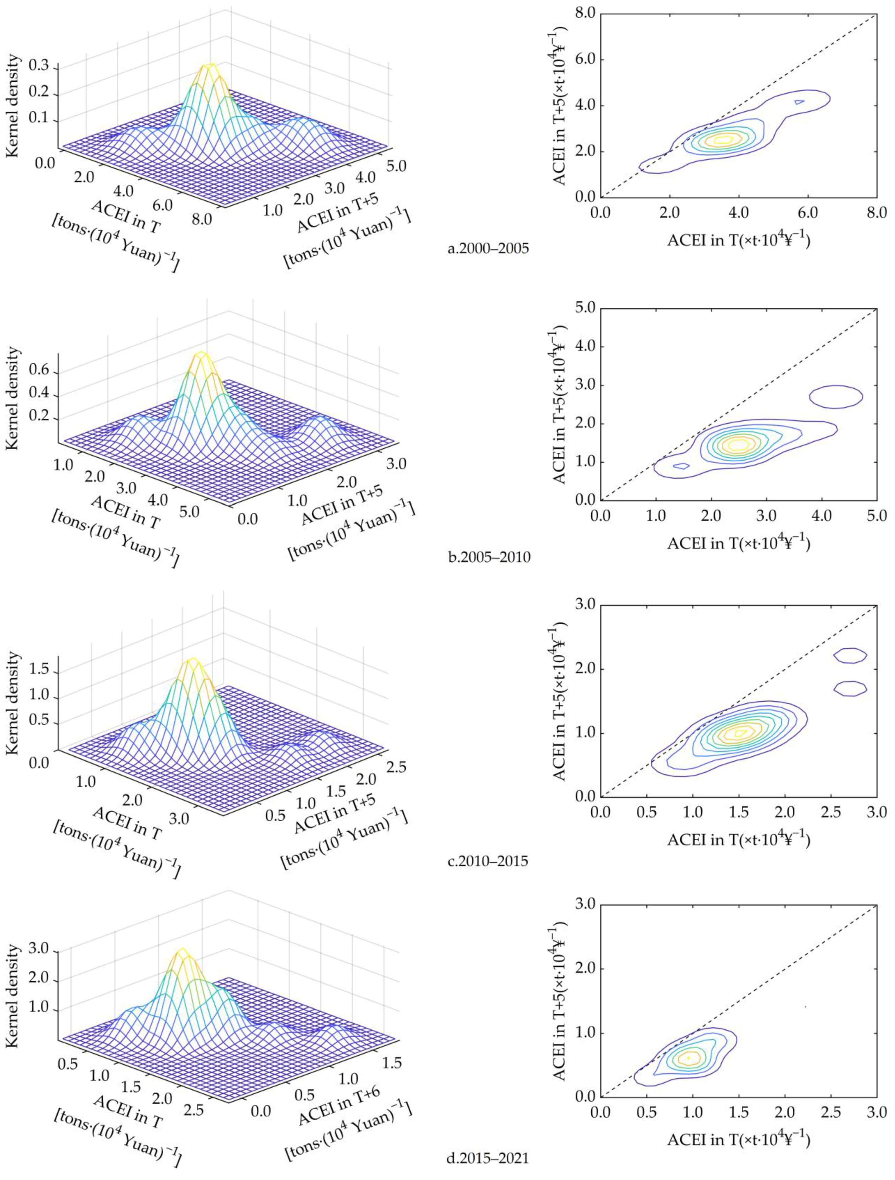
3.2. ACE Dynamic Evolution

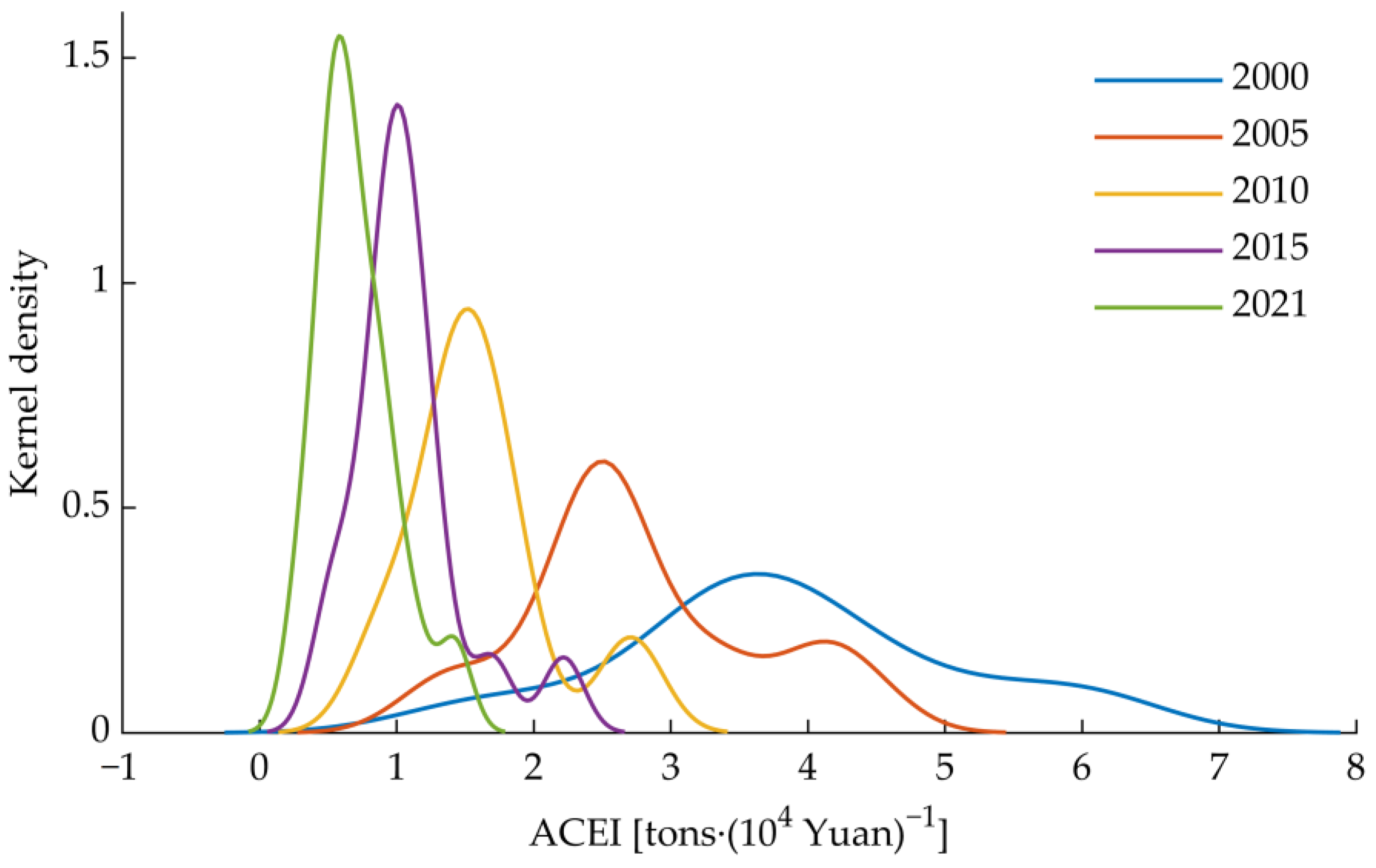
Figure 4 presents the kernel density curves of ACEI in Shandong Province. Examining the curve’s location, interval, and peaks allows us to comprehend the dynamic evolution patterns and spatial disparities of ACEs in the province.

The dynamic evolution of ACEs in Shandong Province’s 16 cities displays two distinct features. First, the center of the distribution curve continuously shifted leftward throughout the study period, while the interval decreased and the peak value gradually increased. This indicates a continuous decrease in ACEI across Shandong Province’s cities, accompanied by a reduction in the disparities of such emissions between them. Secondly, the distribution curve exhibited a single peak in 2000, while a right secondary peak appeared in 2005. Subsequently, the interval and peak value of the right secondary peak gradually decreased until it disappeared completely in 2021, leaving only a slight peak left of the crest. This also suggests decreasing differences in emissions between cities in Shandong Province.

Furthermore, the internal dynamics of the ACE distribution in Shandong Province were examined using conditional probability density estimation. The continuity and mobility of the distribution were analyzed by examining the morphology of stacked conditional density (SCD) plots and density contour (DC) plots.

In Figure 5a, the ridges of the left SCD plots gradually deviate from the 45° diagonal, and most of the density contours of the right DC plots are below the diagonal. This indicates that the distribution of ACEs in Shandong Province from 2000 to 2005 displays a certain degree of mobility. Furthermore, the peak and high-density areas are predominantly below the diagonal, suggesting a gradual decrease in ACEI for most cities, with the potential for further reduction. The cities with ACEI values of [3.4, 6.6] at T + 5 exhibit a more pronounced downward trend and greater mobility, as evidenced by the density contours further away from the diagonal. Conversely, cities with ACEI values of [1.1, 3.4] have density contours close to the diagonal, indicating a lower downward trend and weaker mobility.

In Figure 5b, the ridges and crests of the SCD plots continue to shift below the diagonal, indicating a further increase in the mobility of the ACE distribution in Shandong Province during 2005–2010. The density contours fall entirely below the diagonal, implying a decrease in ACEI for all cities. Notably, a sub-density zone appears in the area corresponding to the ACEI value of [2.3, 3.0] at T + 5, showing a distinct bipolar differentiation in the ACE distribution.

In Figure 5c, the ridges and crests of the SCD plots are still below the diagonal, but a small proportion of the density contours return to the vicinity of the diagonal. This suggests weakened mobility in the distribution of ACEs in Shandong Province during the period of 2010–2015, with a slower decreasing trend of ACEI in each city. At T + 5, the sub-density zone occurs in the areas with ACEI values of [1.6, 1.8] and [2.1, 2.3], indicating a transition from bipolar to multipolar differentiation in the ACE distribution.

In Figure 5d, the ridges and crests of the SCD plots neighbor each other closely and are parallel to the diagonal, while the area of maximum density of the DC plots remains below the diagonal. This indicates a further decline in the mobility of the ACE distribution in Shandong Province during the period of 2015–2021. Despite this, the ACEI of most cities continues to decrease. At T + 6, the sub-density areas concentrate around values of 1.4, indicating the disappearance of ACE distribution polarization in Shandong Province.

3.3. ACE Scenario Projections

The STIRPAT model is widely used to study the drivers of and predict trends in environmental pollution [55]. It decomposes environmental pressures into the combined effects of population size, affluence, and technology level. Based on the theory of the STIRPAT model, we selected seven ACE characteristic variables. These variables collectively reflect the influence of agricultural scale, rural affluence, and agricultural technology level on ACEs. They include rural population, crop sown area, number of large livestock, agricultural industry structure (measured by the ratio of planting output value to total agricultural output value), agricultural GDP per capita, rural per capita disposable income, and total agricultural mechanization power.

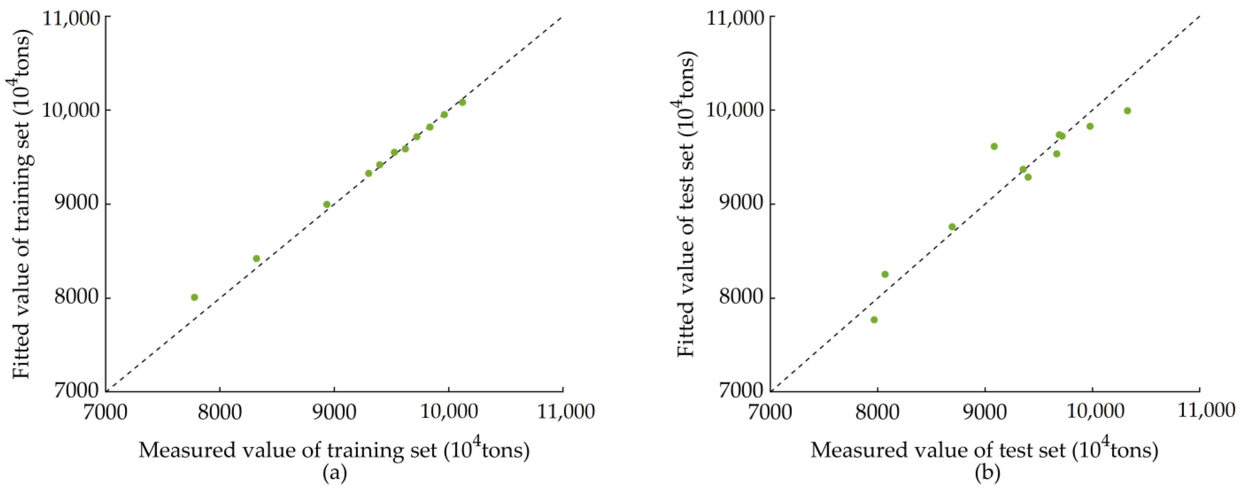
Following the LSTM steps, the sample data were normalized. The training set comprised 11 years of normalized sample data, while the test set used the remaining 11 years. The LSTM’s input layer has a shape of (7, 1), with 50 hidden units in the hidden layer and 1 response in the output layer. To prevent overfitting, a dropout layer with a probability of 0.5 was added. An adaptive momentum estimation optimizer was employed for training the model for 1000 rounds with a batch size of 11. The initial learning rate was 0.01, and a gradient threshold of 1 was applied to prevent gradient explosion. Data were not shuffled during training to preserve temporal order. R² and root mean square error (RMSE) evaluated the LSTM’s fitting effect on the training and test sets. In Figure 6, the training set achieved an R² of 0.9859 and an RMSE of 81.3527, indicating a high fit level. The test set achieved an R² of 0.9079 and an RMSE of 218.1455, suggesting strong generalization ability. This result demonstrates the model’s effectiveness in predicting regional ACEs, with it being further applicable to research.

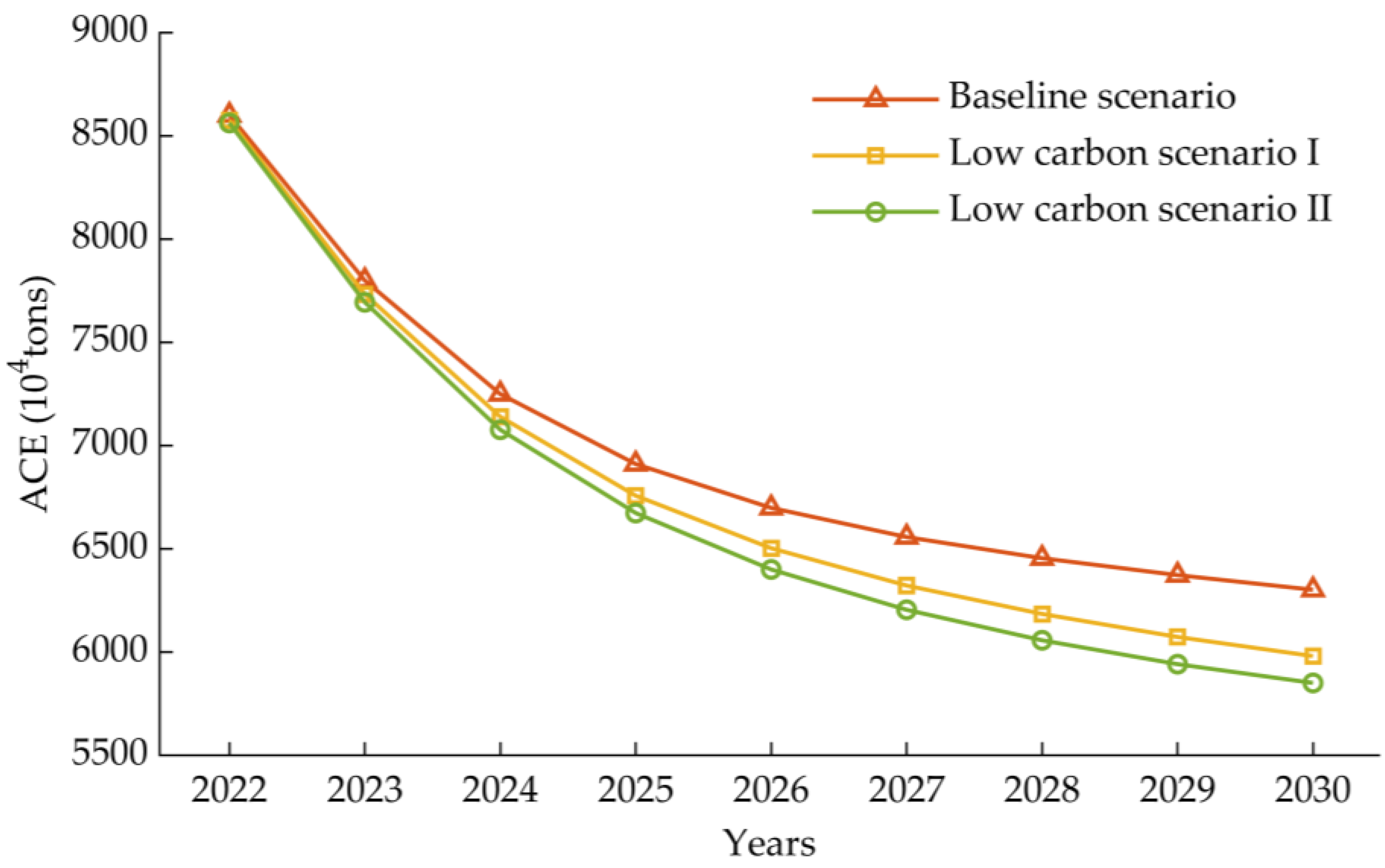
To comprehensively analyze the future trends of ACEs in Shandong Province, three scenarios were established based on the Outline of the Fourteenth Five-Year Plan for the National Economic and Social Development of Shandong Province and the Visionary Goals for 2035 (referred to as the Planning Goals), while considering agriculture development. These scenarios include the baseline scenario, low-carbon scenario I, and low-carbon scenario II.

Several variables are defined for these scenarios. The rural population is determined based on the average annual growth rate of the urbanization rate, set at 1% in the Planning Goals. Agricultural GDP per capita is determined based on the average annual growth rate of GDP, set at 5.5% in the Planning Goals. Rural per capita disposable income is determined based on the average annual growth rate of per capita disposable income, set at 5.5% in the Planning Goals. Crop sown area, number of large livestock, total agricultural mechanization power, and agricultural industrial structure do not have specific development targets in the Planning Goals. Hence, they were set based on the average annual growth rate of the respective sample data. The growth rates of each characteristic variable under different scenarios are shown in

Table 8. The growth rate setting of ACE characteristic variables in Shandong Province under different scenarios.

Scenarios	Years	Growth Rate Setting (%)
		Rural Population	Agricultural GDP per Capita	Rural per Capita Disposable Income	Crop Sown Area	Number of Large Livestock	Total Agricultural Mechanization Power	Agricultural Industrial Structure
Baseline scenario	2022–2025	−1.0	5.5	5.5	−0.0856	6.3954	2.2398	−0.4053
	2026–2030	−1.5	6.0	6.0
Low-carbon scenario I	2022–2025	−3.5	8.0	8.0
	2026–2030	−4.0	8.5	8.5
Low-carbon Scenario II	2022–2025	−5.0	9.5	9.5
	2026–2030	−5.5	10.0	10.0

.

The trained LSTM predicted the ACEs of Shandong Province from 2022 to 2030 under the baseline and low-carbon scenarios, as shown in Figure 7.

In all three scenarios, the ACEs of Shandong Province exhibit a consistent decreasing trend, with the rate of decrease gradually diminishing over the years. In the baseline scenario, the projected value for 2030 is 6301.74 × 10⁴ tons, indicating a 20.91% reduction compared to the 2021 value of 7967.54 × 10⁴ tons. In the low-carbon scenario I, there is a significantly greater decreasing trend in the ACEs compared to the baseline scenario, with a projected value for 2030 at 5980.67 × 10⁴ tons, reflecting a 24.94% decrease from the 2021 value. In the low-carbon scenario II, the ACE decrease rate is the highest among the three scenarios, with a projected value for 2030 at 5850.56 × 10⁴ tons, indicating a 26.57% decrease from the 2021 value. The low-carbon scenario demonstrates a higher potential for reducing carbon emissions while simultaneously achieving efficient development of the rural economy, urbanization, and ACE reduction compared to the baseline scenario.

4. Discussion

4.1. ACE Characteristics of Shandong Province

From 2000 to 2021, ACEs in Shandong Province followed a pattern of initial growth followed by decline, closely associated with China’s agricultural policies. Before 2005, China initiated rural tax reforms while providing subsidies for grain cultivation, high-quality seeds, and agricultural machinery purchases. These agricultural policies effectively incentivized farmers to increase agricultural inputs and expand livestock production. However, during this period, agricultural resources were not utilized optimally, and emission reduction strategies were incomplete, resulting in a significant increase in ACEs. Subsequently, China introduced the concept of environmentally friendly agriculture and implemented a series of measures to reduce ACEs, including actions to achieve zero growth in the use of fertilizers and pesticides. This effectively controlled agricultural input and improved utilization efficiency. Additionally, the annual decline in the rearing volume of large livestock, attributed to the restructuring of the livestock industry and the impact of diseases, contributed to the decrease in ACEs.

Research indicates that carbon emissions from China’s planting industry have surpassed those from the livestock industry [23]. In Shandong Province, carbon emissions from planting accounted for 64.39% of the total emissions primarily originating from soil use and straw burning. To achieve the goal of agricultural carbon neutrality, the province must prioritize reducing emissions and improving efficiency in the planting industry. However, carbon emissions from enteric fermentation and manure management in the livestock industry cannot be overlooked. The livestock industry in Shandong Province is characterized by small-scale operations and a deficiency in standardized feeding management and manure treatment methods, making carbon emissions from this sector still a significant concern.

The primary contributor to agricultural GHG emissions in China is CH₄, followed by CO₂ and N₂O [1]. However, in Shandong Province, CO₂ emerged as the primary GHG emitted, and its distribution is closely related to agricultural production patterns. In 2020, Shandong Province’s ACEI stood at 0.76 × tons∙(10⁴ yuan)⁻¹, marking a notable decrease of 72.46% compared to 2.76 × tons∙(10⁴ yuan)⁻¹ in 2005, surpassing China’s target of reducing carbon emission intensity by 40–45% in 2020. This underscores the remarkable achievement of Shandong Province in ACE reduction. Currently, ACEs in all provinces of China are declining [30,32], and the inter-provincial disparities in ACEs among principal grain-producing areas are narrowing [33]. Nevertheless, for Shandong Province, although ACEI is decreasing, the mobility of ACE distribution has been weakening since 2010, indicating increased pressure for ACE reduction. The diminishing gap in ACEs between cities in Shandong Province is accompanied by a phenomenon of polarization. Although this phenomenon disappeared after 2015, in 2021, 7 out of 16 cities still had ACEIs exceeding the provincial average, indicating persistent emission disparities. Therefore, implementing targeted policies addressing the spatial and temporal differentiation of ACEs in Shandong Province would help establish a coordinated emission reduction pattern across the region.

4.2. Countermeasures to Decrease ACEs in Shandong Province

Shandong Province continues to depend on extensive agricultural production methods that consume resources, and this pattern has not fundamentally changed, leading to a conflict between agricultural development and environmental protection. According to our study, Shandong Province exhibits greater potential for emission reduction under low-carbon scenarios. Therefore, the development of low-carbon, efficient, and sustainable agricultural practices is paramount for achieving emission reduction objectives.

The excessive use of agricultural materials, underutilization of resources, and insufficient technical preparation for the development of green and low-carbon agriculture have resulted in persistently high levels of carbon emissions within the planting industry [56]. The effectiveness of carbon reduction through low-carbon cultivation techniques hinges on the proportion of corresponding carbon sources in ACEs and their implementation level [57]. In Shandong Province, soil utilization and straw burning contribute 34.00% and 22.29% to ACEs, respectively. To curb carbon emissions from planting, it is essential to advocate measures like returning straw to the field, reducing fertilizer and pesticide application while enhancing their efficiency, and adopting agricultural film substitution technologies. Additionally, practices such as crop rotation, intercropping [58], and optimizing intermittent irrigation can further promote carbon emission reduction [59].

Enteric fermentation serves as the primary source of CH₄ emissions from ruminant animals [60]. In Shandong Province, enteric fermentation and manure management in livestock contribute 22.86% and 12.75% to ACEs, respectively. Effective strategies to mitigate carbon emissions from livestock encompass optimizing feed composition, improving barn environments, adjusting breeding structures, and properly utilizing livestock manure. Intensive, standardized, and large-scale farming practices can reduce enteric fermentation in livestock while increasing the efficiency of manure management, thereby facilitating the return of livestock manure to fields. Moreover, curtailing livestock product consumption represents an effective measure to alleviate non-CO₂ GHG emissions [61].

5. Conclusions

(1)

Between 2000 and 2021, Shandong Province achieved remarkable progress in reducing ACEs, reaching its agricultural carbon peak in 2005. ACEs are structured as “soil utilization > enteric fermentation > straw burning > manure management > crop planting “, with the planting industry serving as the primary emissions source. The GHG composition follows “CO₂ > CH₄ > N₂O”, with emission distribution closely linked to regional agricultural production modes. CO₂ emissions are mainly distributed in crop cultivation areas, whereas CH₄ and N₂O emissions are primarily concentrated in livestock breeding areas. The emission inventory provides a precise representation of ACE characteristics, but it is not without uncertainty, primarily arising from emission factors. To reduce the uncertainty of the emission inventory, future research should focus on intensifying the localization of emission factors from major sources.

(2)

Between 2000 and 2021, the ACEI of different cities in Shandong province exhibited a declining trend, indicating a decoupling between ACEs and agricultural economic growth. Although spatial imbalances persist, the emission disparity among cities is diminishing. Nevertheless, the mobility of ACE distribution is gradually decreasing, posing a challenge to further mitigating ACEs.

(3)

From 2022 to 2030, the ACEs in Shandong Province will continue to decline. The low-carbon scenario has greater potential for carbon emissions reduction compared to the baseline scenario. It also balances efficient development of the rural economy and urbanization, thereby accelerating the achievement of the province’s “dual carbon” goals.

6. Suggestions

(1)

Establish a comprehensive monitoring and evaluation system for ACEs. Improve monitoring indicators, localize emission factors, unify measurement methods, optimize the setup of monitoring points in different regions, and conduct targeted monitoring alongside regular statistical analysis.

(2)

Strengthen the prevention and control of agricultural surface source pollution. Promote techniques such as soil testing for tailored fertilization, organic fertilizers replacing chemical ones, and biological and physical methods of pest control, aiming to reduce the use of chemical fertilizers and pesticides while enhancing agricultural productivity. Establish systems for the collection, storage, and transportation of agricultural waste to facilitate the efficient utilization of resources such as livestock manure, straw, and agricultural film.

(3)

Optimize the agricultural industry structure and establish a new agricultural production pattern that matches agricultural productivity with the carrying capacity of resources and the environment. In the central and southern regions of Shandong Province, where resource overexploitation and environmental issues are prominent, adjust the crop and livestock structure, and implement land retirement for afforestation to promote integrated crop–livestock. In areas with better alignment of agricultural production with water and soil resources, such as Weihai, Rizhao, and Dongying, develop forestry, fisheries, and ecological agriculture tourism industries with comparative advantages and regional characteristics.

(4)

Building a green and low-carbon agricultural industry chain to increase agricultural GDP and the income of rural residents. Promote variety cultivation and standardized production to enhance the quality of agricultural products. Simultaneously, constructing a green supply chain for agricultural products will drive industrial clustering and circular development. These measures will lead Shandong Province’s agricultural development into a low-carbon scenario.

References

1. Fan, Z.Y.; Qi, X.B.; Zeng, L.L.; Wu, F. Accounting of greenhouse gas emissions in the Chinese agricultural system from 1980 to 2020. Acta Ecol. Sin. 2022, 44, 9470–9482. [Google Scholar] [CrossRef]
2. IPCC. Mitigation of Climate Change. Contribution of Working Group III to the Fourth Assessment Report of the Intergovernmental Panel on Climate Change Cambridge; Climate Change 2007; Cambridge University Press: London, UK, 2007. [Google Scholar]
3. Tubiello, F.N.; Salvatore, M.; Rossi, S.; Ferrara, A.; Fitton, N.; Smith, P. The FAOSTAT database of greenhouse gas emissions from agriculture. Environ. Res. Lett. 2013, 8, 015009. [Google Scholar] [CrossRef]
4. Johnson, J.M.F.; Franzluebbers, A.J.; Weyer, S.L.; Reicosky, D.C. Agricultural opportunities to mitigate greenhouse gas emissions. Environ. Pollut. 2007, 150, 107–124. [Google Scholar] [CrossRef] [PubMed]
5. Lin, B.Q.; Fei, R.L. Regional differences of CO2 emissions performance in China’s agricultural sector: A Malmquist index approach. Eur. J. Agron. 2015, 70, 33–40. [Google Scholar] [CrossRef]
6. West, T.O.; Marland, G. A synthesis of carbon sequestration, carbon emissions, and net carbon flux in agriculture: Comparing tillage practices in the United States. Agric. Ecosyst. Environ. 2002, 91, 217–232. [Google Scholar] [CrossRef]
7. Lal, R. Carbon emission from farm operations. Environ. Int. 2004, 30, 981–990. [Google Scholar] [CrossRef]
8. Li, B.; Zhang, J.B.; Li, H.P. Research on Spatial-temporal Characteristics and Affecting Factors Decomposition of Agricultural Carbon Emission in China. Chin. J. Popul. Resour. Environ. 2011, 21, 80–86. [Google Scholar] [CrossRef]
9. Cheng, K.; Pan, G.; Smith, P.; Luo, T.; Li, L.; Zheng, J.; Zhang, X.; Han, X.; Yan, M. Carbon footprint of China’s crop production—An estimation using agro-statistics data over 1993–2007. Agric. Ecosyst. Environ. 2011, 142, 231–237. [Google Scholar] [CrossRef]
10. Norse, D. Low carbon agriculture: Objectives and policy pathways. Environ. Dev. 2012, 1, 25–39. [Google Scholar] [CrossRef]
11. Linquist, B.A.; Adviento-Borbe, M.A.; Pittelkow, C.M.; van Kessel, C.; van Groenigen, K.J. Fertilizer management practices and greenhouse gas emissions from rice systems: A quantitative review and analysis. Field Crops Res. 2012, 135, 10–21. [Google Scholar] [CrossRef]
12. Gangopadhyay, S.; Banerjee, R.; Batabyal, S.; Das, N.; Mondal, A.; Pal, S.C.; Mandal, S. Carbon sequestration and greenhouse gas emissions for different rice cultivation practices. Sustain. Prod. Consump. 2022, 34, 90–104. [Google Scholar] [CrossRef]
13. Aguilera, E.; Lassaletta, L.; Sanz-Cobena, A.; Garnier, J.; Vallejo, A. The potential of organic fertilizers and water management to reduce N2O emissions in Mediterranean climate cropping systems. A review. Agric. Ecosyst. Environ. 2013, 164, 32–52. [Google Scholar] [CrossRef]
14. Spawn, S.A.; Lark, T.J.; Gibbs, H.K. Carbon emissions from cropland expansion in the United States. Environ. Res. Lett. 2019, 14, 045009. [Google Scholar] [CrossRef]
15. Sun, J.; Peng, H.; Chen, J.; Wang, X.; Wei, M.; Li, W.; Yang, L.; Zhang, Q.; Wang, W.; Mellouki, A. An estimation of CO2 emission via agricultural crop residue open field burning in China from 1996 to 2013. J. Clean. Prod. 2016, 112, 2625–2631. [Google Scholar] [CrossRef]
16. Romasanta, R.R.; Sander, B.O.; Gaihre, Y.K.; Alberto, M.C.; Gummert, M.; Quilty, J.; Nguyen, V.H.; Castalone, A.G.; Balingbing, C.; Sandro, J.; et al. How does burning of rice straw affect CH4 and N2O emissions? A comparative experiment of different on-field straw management practices. Agric. Ecosyst. Environ. 2017, 239, 143–153. [Google Scholar] [CrossRef]
17. Havlík, P.; Valin, H.; Herrero, M.; Obersteiner, M.; Schmid, E.; Rufino, M.C.; Mosnier, A.; Thornton, P.K.; Böttcher, H.; Conant, R.T.; et al. Climate change mitigation through livestock system transitions. Proc. Natl. Acad. Sci. USA 2014, 111, 3709–3714. [Google Scholar] [CrossRef] [PubMed]
18. Garnier, J.; Le, J.; Marescaux, A.; Sanz-Cobena, A.; Lassaletta, L.; Silvestre, M.; Thieu, V.; Billen, G. Long-term changes in greenhouse gas emissions from French agriculture and livestock (1852–2014): From traditional agriculture to conventional intensive systems. Sci. Total. Environ. 2019, 660, 1486–1501. [Google Scholar] [CrossRef] [PubMed]
19. Zhou, Y.F.; Li, B.; Zhang, Y.Q. Spatiotemporal evolution and influencing factors of agricultural carbon emissions in Hebei Province at the county scale. Chin. J. Eco-Agric. 2022, 30, 570–581. [Google Scholar] [CrossRef]
20. Dalgaard, T.; Olesen, J.E.; Petersen, S.O.; Petersen, B.M.; Jørgensen, U.; Kristensen, T.; Hutchings, N.J.; Gyldenkærne, S.; Hermansen, J.E. Developments in greenhouse gas emissions and net energy use in Danish agriculture–How to achieve substantial CO2 reductions? Environ. Pollut. 2011, 159, 3193–3203. [Google Scholar] [CrossRef]
21. Han, H.B.; Zhong, Z.Q.; Guo, Y.; Xi, F.; Liu, S.L. Coupling and decoupling effects of agricultural carbon emissions in China and their driving factors. Environ. Sci. Pollut. Res. 2018, 25, 25280–25293. [Google Scholar] [CrossRef]
22. Wu, H.; Huang, H.; Chen, W.; Meng, Y. Estimation and spatiotemporal analysis of the carbon-emission efficiency of crop production in China. J. Clean. Prod. 2022, 371, 133516. [Google Scholar] [CrossRef]
23. Zeng, X.G.; Yu, C.; Sun, Y.Q. Carbon emission structure and carbon peak of agriculture and rural areas in China. China Environ. Sci. 2023, 43, 1906–1918. [Google Scholar] [CrossRef]
24. Elżbieta, W.G.; Marta, B.M. Assessment of greenhouse gas emission from life cycle of basic cereals production in Poland. Zemdirbyste 2016, 103, 259–266. [Google Scholar] [CrossRef]
25. Yadav, D.; Wang, J.Y. Modelling carbon dioxide emissions from agricultural soils in Canada. Environ. Pollut. 2017, 230, 1040–1049. [Google Scholar] [CrossRef] [PubMed]
26. Qiu, Z.J.; Jin, H.M.; Gao, N.; Xu, X.; Zhu, J.H.; Li, Q.; Wang, Z.Q.; Xu, Y.J.; Shen, W.S. Temporal characteristics and trend prediction of agricultural carbon emission in Jiangsu Province, China. J. Agro-Environ. Sci. 2022, 41, 658–669. [Google Scholar] [CrossRef]
27. Gu, R.; Duo, L.; Guo, X.; Zou, Z.; Zhao, D. Spatiotemporal heterogeneity between agricultural carbon emission efficiency and food security in Henan, China. Environ. Sci. Pollut. Res. 2023, 30, 49470–49486. [Google Scholar] [CrossRef] [PubMed]
28. Zhang, X.; Liao, K.; Zhou, X. Analysis of regional differences and dynamic mechanisms of agricultural carbon emission efficiency in China’s seven agricultural regions. Environ. Sci. Pollut. Res. 2022, 29, 38258–38284. [Google Scholar] [CrossRef]
29. Zhu, Y.B.; Ma, X.Z.; Shi, Y.J. Agricultural input-output efficiency and the potential reduction of emissions in Henan Province at the county scale Chinese. J. Eco-Agric. 2022, 30, 1852–1861. [Google Scholar] [CrossRef]
30. Yuan, Y.; Sun, X.T. Spatial-temporal Evolution and Driving Factors of Inter-provincial Carbon Emission Intensity in China. Environ. Sci. Technol. 2022, 45, 168–176. [Google Scholar] [CrossRef]
31. Guo, H.; Fan, B.; Pan, C. Study on Mechanisms Underlying Changes in Agricultural Carbon Emissions: A Case in Jilin Province, China, 1998–2018. Int. J. Environ. Res. Public Health 2021, 18, 919. [Google Scholar] [CrossRef]
32. Wu, G.Y.; Liu, J.D.; Yang, L.S. Dynamic evolution of China’s agricultural carbon emission intensity and carbon offset potential. China Popul. Resour. Environ. 2021, 31, 69–78. [Google Scholar] [CrossRef]
33. Tian, Y.; Yin, M.H. Re-evaluation of China’s Agricultural Carbon Emissions: Basic Status, Dynamic Evolution and Spatial Spillover Effects. Chin. Rural. Econ. 2022, 3, 104–127. [Google Scholar]
34. Jiang, J.; Zhao, T.; Wang, J. Decoupling analysis and scenario prediction of agricultural CO2 emissions: An empirical analysis of 30 provinces in China. J. Clean. Prod. 2021, 320, 128798. [Google Scholar] [CrossRef]
35. Wang, S.F.; Gao, G.L.; Li, W.; Liu, S.M. Carbon emissions from agricultural and animal husbandry in Shanxi Province: Temporal and regional aspects, and trend forecast. J. Agro-Environ. Sci. 2023, 42, 1–18. [Google Scholar] [CrossRef]
36. Xiao, X.W.; Liu, X.H.; Liu, Z.S.; Qin, H.M.; Li, S.; Zhang, Y.L.; Chen, X.X. Characteristics, driving factors and trend prediction of agriculture carbon emission in the three gorges reservoir area. (Hubei Section). Chin. J. Agric. Resour. Reg. Plan. 2023, 44, 212–222. [Google Scholar]
37. Chang, Q.; Cai, W.M.; Gu, X.L.; Wu, Y.Q.; Zhang, B.L. Spatial-Temporal Variation, Influencing Factors, and Trend Prediction of Agricultural Carbon Emissions in Henan Province. Bull. Soil. Water Conserv. 2023, 43, 367–377. [Google Scholar] [CrossRef]
38. Xu, L.; Qu, J.S.; Wu, J.J.; Wei, Q.; Bai, J.; Li, H.J. Spatial-Temporal Dynamics and Prediction of Carbon Emission from Agriculture and Animal Husbandry in China. J. Ecol. Rural. Environ. 2019, 35, 1232–1241. [Google Scholar] [CrossRef]
39. Wei, Z.; Wei, K.; Liu, J.; Zhou, Y.Z. The relationship between agricultural and animal husbandry economic development and carbon emissions in Henan Province, the analysis of factors affecting carbon emissions, and carbon emissions prediction. Mar. Pollut. Bull. 2023, 193, 115134. [Google Scholar] [CrossRef]
40. IPCC. Synthesis Report. Contribution of Working Groups I, II and III to the Fifth Assessment Report of the Intergovernmental Panel on Climate Change; Climate Change, 2014; Pachauri, R.K., Meyer, L.A., Eds.; IPCC: Geneva, Switzerland, 2014; p. 151. [Google Scholar]
41. Zhang, S.Y.; Yin, C.J.; He, Y.Y.; Xiao, X.Y. Spatial differentiation and dynamic evolution of agricultural carbon emission in China—Empirical research based on spatial and non-parametric estimation methods. China Environ. Sci. 2020, 40, 1356–1363. [Google Scholar] [CrossRef]
42. Tian, Y.; Zhang, J.B.; He, Y.Y. Research on Spatial-Temporal Characteristics and Driving Factor of Agricultural Carbon Emissions in China. J. Integr. Agric. 2014, 13, 1393–1403. [Google Scholar] [CrossRef]
43. Zhi, J.; Gao, J.X. Analysis of carbon emission caused by food consumption in urban and rural inhabitants in China. Prog. Geogr. 2009, 28, 429–434. [Google Scholar]
44. Wu, F.L.; Li, L.; Zhang, H.L.; Chen, F. Effects of conservation tillage on net carbon flux from farmland ecosystems. Chin. J. Ecol. 2007, 26, 2035–2039. [Google Scholar] [CrossRef]
45. National Development and Reform Commission, PRC. Guidelines for the Preparation of Provincial Greenhouse Gas Inventories (Trial). Available online: http://www.gxdtrc.cn/h-nd-217.html (accessed on 16 May 2023).
46. Min, J.S.; Hu, H. Calculation of Greenhouse Gases Emission from Agricultural Production in China. China Popul. Resour. Environ. 2012, 22, 21–27. [Google Scholar] [CrossRef]
47. Liu, Y.; Liu, H.B. Characteristics, influence factors, and prediction of agricultural carbon emissions in Shandong Province. Chin. J. Eco-Agric. 2022, 30, 448–569. [Google Scholar] [CrossRef]
48. Xie, Y.H.; Liu, Z. Study on Spatial Spillover Effect and Equity of Planting Carbon Emission in Henan Province at County Scale. Areal Res. Dev. 2022, 41, 159–164. [Google Scholar] [CrossRef]
49. Hu, X.D.; Wang, J.M. Estimation of livestock greenhouse gases discharge in China. Trans. Chin. Soc. Agric. Eng. 2010, 26, 247–252. [Google Scholar] [CrossRef]
50. Mood, A.M. An Introduction to the Theory of Statistics; McGraw-Hill Book Company: New York, NY, USA, 1973. [Google Scholar]
51. Silverman, B.W. Density Estimation for Statistics and Data Analysis; Chapman and Hall: London, UK, 1986. [Google Scholar]
52. Hyndman, R.J.; Bashtannyk, D.M.; Grunwald, G.K. Estimating and visualizing conditional densities. J. Comput. Graph. Stat. 1996, 5, 315–336. [Google Scholar] [CrossRef]
53. Hochreiter, S.; Schmidhuber, J. Long short-term memory. Neural Comput. 1997, 9, 1735–1780. [Google Scholar] [CrossRef]
54. Graves, A. Supervised Sequence Labelling with Recurrent Neural Networks; Springer: Berlin/Heidelberg, Germany, 2012. [Google Scholar]
55. Ma, H.; Liu, Y.; Li, Z.; Wang, Q. Influencing factors and multi-scenario prediction of China’s ecological footprint based on the STIRPAT model. Ecol. Inform. 2022, 69, 101664. [Google Scholar] [CrossRef]
56. Wang, X.T.; Zhang, J.B. Basic path and system construction of agricultural green and low-carbon development with respect to the strategic target of carbon peak and carbon neutrality. Chin. J. Eco-Agric. 2022, 30, 516–526. [Google Scholar] [CrossRef]
57. Huang, B.B.; Zhang, X.Y.; Zhang, J.Q. Carbon Reduction Effect and Application Drivers of Low-Carbon Planting Technologies. J. Ecol. Rural. Environ. 2018, 34, 1082–1090. [Google Scholar] [CrossRef]
58. Wang, Y.; Yang, D.L.; Wang, L.L.; Zhao, J.N.; Liu, H.M.; Tan, B.C.; Wang, H.; Wang, M.L.; Huang, J.; Zhang, X.F. Effects of farmland management measures on soil organic carbon turnover and microorganisms. J. Agric. Resour. Environ. 2020, 37, 340–352. [Google Scholar] [CrossRef]
59. Zhang, D.; Shen, J.; Zhang, F.; Li, Y.E.; Zhang, W. Carbon footprint of grain production in China. Sci. Rep. 2017, 7, 4126. [Google Scholar] [CrossRef] [PubMed]
60. Wang, K.Y.; Li, X.; Lu, J.D.; Zhou, B.; He, Y. Low-carbon development strategies of livestock industry to achieve goal of carbon neutrality in China. Trans. Chin. Soc. Agric. Eng. 2022, 38, 230–238. [Google Scholar] [CrossRef]
61. Frank, S.; Havlík, P.; Stehfest, E.; van Meijl, H.; Witzke, P.; Domínguez, I.P.; van Dijk, M.; Doelman, J.C.; Fellmann, T.; Koopman, J.F.L.; et al. Agricultural non-CO2 emission reduction potential in the context of the 1.5 C target. Nat. Clim. Change 2019, 9, 66–72. [Google Scholar] [CrossRef]
Figure 1. Geographical location, administrative divisions, and land use types in Shandong Province.
Sustainability 16 03196 g001
Figure 2. Emission structure of agricultural CH4 (a), N2O (b), CO2 (c), and total emissions (d) in Shandong Province from 2000 to 2021. Note: The subscripts ch, sh, eh, and mh represent CH4 emissions from crop planting, straw burning, enteric fermentation, and manure management, respectively. The subscripts cn, ni, nd, lr, and mn represent N2O emissions from crop planting, in-season nitrogen inputs to agricultural land, atmospheric nitrogen deposition, nitrogen loss through leaching and runoff, and livestock manure management, respectively. The subscript sc represents CO2 emissions from straw burning.
Sustainability 16 03196 g002
Figure 3. Emission inventory of agricultural CH4, N2O, CO2, and total emissions in Shandong Province at 1 km × 1 km resolution for the period of 2000 to 2021.
Sustainability 16 03196 g003
Figure 4. Kernel density estimate curves of ACEI in Shandong Province from 2000 to 2021.
Sustainability 16 03196 g004
Figure 5. Stacked conditional density plots and density contour plots of ACEI in Shandong Province from 2000 to 2021.
Sustainability 16 03196 g005
Figure 6. Comparison of fitted and measured values of ACEs for the LSTM training set (a) and test set (b).
Sustainability 16 03196 g006
Figure 7. Prediction values of ACEs for Shandong Province from 2022 to 2030 under different scenario models.
Sustainability 16 03196 g007