Two-Layer Optimization Strategy of Electric Vehicle and Air Conditioning Load Considering the Benefit of Peak-to-Valley Smoothing

Abstract

To satisfy the interests of multiple agents and those of comprehensive indicators such as peak-to-valley differences and load fluctuations occurring on the network side, this paper presents a flexible load demand-side response optimization method that considers the benefits of peak-to-valley smoothing. First, load aggregation modelling of air conditioning and electric vehicles was conducted, and the complementarity of the power consumption behavior of different types of flexible loads was used to improve the responsiveness of the load aggregator. Second, considering demand-side responses and taking into account the interests of both supply and demand, the load fluctuation and peak-to-valley difference on the network side are reduced, and a flexible load double-layer optimization model incorporating the peak-to-valley smoothing benefit is established. Finally, the effectiveness of the proposed optimization model is verified by using the KKT condition and the big M method to evaluate this two-layer optimization problem as a single-layer optimization problem. Comparative examples show that the proposed two-layer optimization method can take advantage of the complementarity of air conditioning and electric vehicles to improve the income of load aggregators. Moreover, the proposed method can effectively reduce the load peak-to-valley difference and load fluctuation of the distribution network by introducing the peak-to-valley smoothing benefit model.

1. Introduction

Under the goal of “double carbon”, the construction of a new type of power system that adapts to the gradual increase in the proportion of new energy that is renewable is the key to building an energy system of the future [1]. As the output of renewable energy is significantly affected by weather factors, there is volatility and stochasticity, related power systems face an increased risk of double imbalances of short-term power and long-term power [2]. Energy users have a large number of adjustable flexible load resources, and relying on demand response (DR) and related means can promote power grid peak cutting, valley filling, and renewable energy consumption. Therefore, the use of demand-side flexible loads to achieve source–load interaction is an important development direction for new power systems to achieve supply–demand balance.

Air conditioning (AC) and electric vehicles (Evs) are typical flexible loads that have great potential for being adjusted. During high summer temperatures, air conditioning system loads can reach more than 30% of the grid peak load. Simultaneously, the number of electric vehicles in China has exceeded 14.01 million [3,4,5]. Because air conditioning and electric vehicle loads are large, reasonable regulation measures can effectively alleviate the power supply tension incurred by using such equipment and ensure the safe and stable operation of the power grid. Working on efficient energy management solutions in buildings, especially for HVAC systems, leads to significant economic, social, and environmental improvements [6,7]. For example, aiming at the problem that direct load control of temperature-controlled loads usually affects customer comfort and makes itdifficult to consider responsiveness, the authors of [8] proposed a method of air-conditioning load aggregation operation control and demand response for power sales companies. From the perspective of the power sales company, a temperature-controlled load compensation mechanism is constructed to promote user participation in demand response. Reference [9], based on the pricing strategy of electric vehicle charging based on the quality of service, designed a package model with different quality of service, which effectively reduces the user’s charging cost. Due to diversity in types and decentralized integration of AC load, the dispatch center faces challenges in directly accessing its aggregated power and conducting scheduling control, limiting the full potential of its response. To address this issue, the authors of [10] proposed a dual-layer control framework that combines multiple types of resources, considering the aggregation response potential of air conditioning load, and integrates precise control into the scheduling process. Reference [11] divided the user group into five groups according to the different sensitivities of different users to the temperature to propose an air conditioning scheduling strategy based on the user’s differentiated comfort, and finally verified the strategy through arithmetic example analysis to complete the new energy consumption based on the new energy and, at the same time, to ensure the comfort of the users.

Reference [12], considering the specific models of heat load and battery degradation, proposed practical and flexible MEBM operation model which rigorously models the interdependence between EV load and household appliances. Reference [13] introduces a rolling optimization scheduling mechanism based on real-time data collection, processing, and analysis. This allows our approach to deal with the uncertain availability of electric vehicles. Reference [14] introduces a dynamic carbon emission factor to integrate the total cost of the system (including electricity and carbon emission costs) and user comfort as multiple objectives to optimize air conditioning operation with a single objective. Reference [15] establishes a polymeric model of air conditioning to increase the potential of users to participate in demand response by changing the temperature rise compensation factor. Reference [16], considering interactions with Distribution System Operators (DSOs) and EV users, developed a novel multi-phase joint tendering and pricing strategy for EVA. Reference [17] proposes a dynamic dual-level distribution network optimization scheduling method based on carbon emission factor considering friendly interaction with electric vehicles, which effectively reduces carbon emissions and improves the income of electric vehicle load aggregators. There have been studies on the demand-side response of air conditioning loads and electric vehicle loads, but most of these studies only model and regulate a single flexible load, and few studies have considered the complementarity of the joint optimization of different flexible loads.

The optimal operation of grid flexible loads usually Involves the participation of multiple subjects, and the interests of multiple subjects need to be considered. Reference [18] proposed a tri-level optimization problem that seeks the maximization of revenues from Distributed Energy Resources, the optimization problem considers Electric Vehicles, Battery Energy Storage Systems and Heating, and Ventilation and Air Conditioning in national and local markets. Reference [19] describes a home energy-management system incorporating HVAC and EV that optimally schedules behind-the-meter resources under a tariff with an export rate and analyzes the operation of each behind-the-meter resource and the impact on homeowners’ costs and comfort levels. In Reference [20], a two-stage energy management strategy for the contribution of PEVs in demand response programs of commercial building microgrids is addressed to reduce the on-peak demand, improve the economic efficiency, and increase the environmental sustainability. In reference [21], EV and HVAC aggregator models are developed to represent the fleet of grid-interactive efficient buildings, then a tri-Ievel bidding and dispatching framework is established based on competitive distribution operation with distribution locational marginal price, which satisfies the interests of load aggregators and distribution network operators simultaneously. The above literature mainly focuses on the interests of multiple subjects in the demand-side response process, but fails to consider peak shaving and valley filling on the distribution network side, which may lead to the phenomenon of “adding peaks to peaks” [22].

In summary, the existing demand-side response studies for user flexible loads are still mainly focused on the modelling and analysis of single flexible loads; although the interests of the upper and lower layers are considered in the constructed two-tier optimal operation model, comprehensive indicators such as peak-to-valley differences and load fluctuations on the distribution network side are lacking. Therefore, this paper presents a flexible load demand-side response optimization method that considers the benefits of peak–valley smoothing. First, the loads of the air conditioner and electric vehicle are modelled to improve the response ability of the load aggregator by using the complementary nature of different types of flexible loads. Second, taking into account the benefits of both the supply and demand sides in the process of demand-side response, the load fluctuation and the peak–valley difference on the network side are reduced, and a two-layer optimization model of flexible load is established considering the benefits of peak–valley smoothing. Finally, the two-layer optimization problem is transformed into a single-layer optimization problem by the KKT condition and large M method, and the effectiveness of the proposed optimization model is verified.

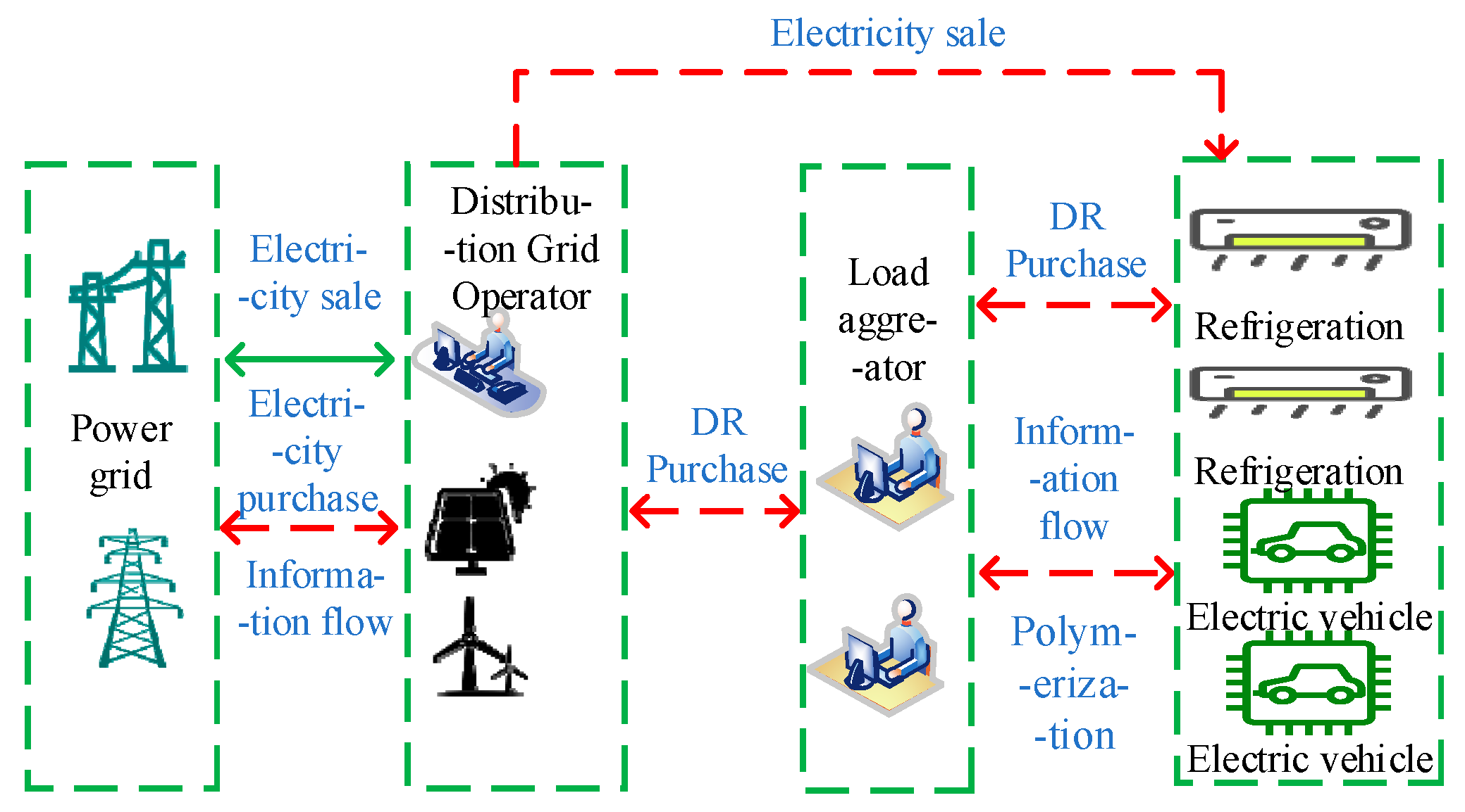
2. Flexible Load Demand Side Response Architecture

The operational architecture of the proposed two-tier optimization model for distribution networks with flexible loads constructed is shown in Figure 1. The load aggregator enters into an agreement with the platform users who can participate in load regulation. This load aggregator controls air conditioning loads and electric vehicle charging loads through terminal equipment connected to the air conditioner, electric vehicle charging posts, etc. The multiple subjects involved in the two-tier model for flexible load optimization are defined as follows:

(1)

Distribution system operator (DSO).

The upper DSO needs to consider its own net profit from selling electricity and purchasing electricity, and it obtains its own income by selling electricity to users. To improve the revenue of the DSO and meet the electricity demand of users, the DSO needs to interact with load aggregators and external power grids. The grid decides the amount of electricity to be traded with the DSO through the DSO’s day-ahead information interaction. When there is a surplus of electricity, revenue can also be gained by selling electricity to the grid at a low price.

(2)

Load aggregator (LA).

As a bridge between the DSO and users, the LA improves the enthusiasm of users to participate in demand response through measures such as electricity price and incentives. To satisfy the user’s own energy demand, the LA integrates flexible load response resources, and sells its aggregated adjustable resources to the DSO to achieve its own dispatch revenue.

(3)

Users with flexible loads.

The flexible load users mainly include electric vehicle owners and air conditioning operators. By signing an agreement with the user, the load aggregator uses the intelligent terminal installed on the air conditioner to control the temperature setting of the air conditioner and the charging pile to control the charging time of the user’s electric vehicle.

3. Flexible Load Resource Aggregation Models

3.1. Aggregation Modelling of the Air Conditioning Load

Air conditioning load modelling currently uses the equivalent thermal parameter model (ETP). The ETP model can be divided into first-order and second-order models. [23,24] To simplify the model complexity, this paper adopts the first-order ETP model to describe the thermodynamic process of the air conditioning unit, and the relationship between the air conditioning power and the indoor and outdoor temperatures is shown in Equation (1) [25]:

$$C\frac{d{T}_{in}^t}{dt}=\frac{T_{out}^t-T_{in}^t}{R}-{\eta }_{ac}u\left(t\right)P_{ac}^t$$

(1)

where $T_{in}^t$ and $T_{out}^t$ are the indoor temperature and outdoor temperature at moment t, respectively; $P_{ac}^t$ is the electric power of air conditioning at moment t; R is the equivalent thermal resistance of the wall; C is the equivalent heat capacity of the air conditioning; $u\left(t\right)$ is the operating state of the air conditioning; and ${\eta }_{ac}$ is the ratio of air conditioning energy consumption. Assuming that the air conditioner is in thermal steady-state operation, the set temperature of the air conditioner is $T_{set}^t$ = $T_{in}^t$; because $d{T}_{in}^t/dt=0$, we can obtain a single air conditioner that consumes electric power $P_{ac}^t$:

$$P_{ac}^t=\frac{T_{out}^t-T_{in}^t}{\eta R}$$

(2)

Assuming that there are N air conditioners, the total power of the air conditioning unit can be estimated based on the power of a single air conditioner as follows:

$$\begin{array}{ll}{P}_{AC}^t=& {\displaystyle \sum _{n=1}^N{P}_{ac}^t\approx {\displaystyle \sum _{n=1}^N\frac{T_{out}^t-T_{in}^t}{{\eta }_n{R}_n}}}\\ & T_{\min }^t\le T_{\mathrm{in}}^t\le T_{\max }^t\end{array}$$

(3)

$$\Delta P_{AC.d}^t=P_{AC}^t-P_{AC}^{lit}$$

(4)

$$P_{AC}^{lit,t}={\displaystyle \sum _{n=1}^N\frac{T_{out}^t-T_{\max }^t}{{\eta }_n{R}_n}}$$

(5)

where $P_{HVAC}^t$ is the aggregated power of N air conditioners at time t; $\Delta P_{HVAC.d}^t$ is the upper limit of the cut power of N air conditioner loads at time t; $P_{HVAC}^{lit,t}$ is the aggregated power of the user at the highest tolerable indoor temperature; and $T_{\min }^t$, $T_{\max }^t$ is the range of temperature comfort required to satisfy the user’s comfort level.

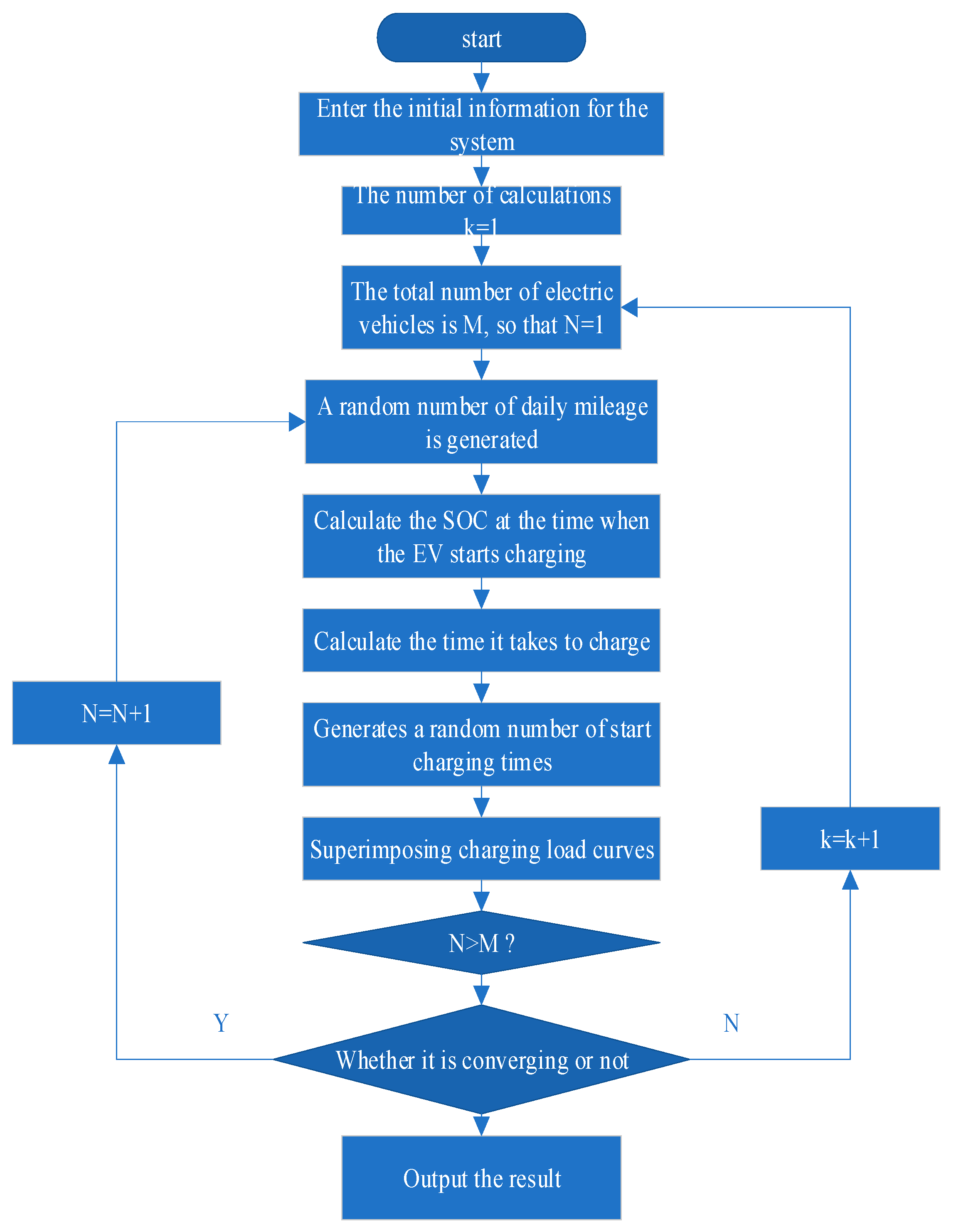
3.2. Aggregation Modelling of Electric Vehicles

A mature method for modelling electric vehicle (EV) loads is currently the Monte Carlo method. It uses the U.S. Household Travel Survey to model the start and end times of EV charging:

$$f_s\left(t\right)=\{\begin{array}{l}\frac{1}{\sqrt{2}{\sigma }_s}\exp \left(-\frac{{\left(t+24-{\mu }_s\right)}^2}{2{\sigma }_s^2}\right),0<t\le \left({\mu }_s-12\right)\\ \frac{1}{\sqrt{2}\pi {\sigma }_s}\exp \left(-\frac{{\left(t-{\mu }_s\right)}^2}{2{\sigma }_s^2}\right),{\mu }_s-12<t\le 24\end{array}$$

(6)

where $f_s\left(t\right)$ is the probability density function of the electric vehicle at the start of charging, $u_s$ is the expectation of the probability density function, and ${\sigma }_s$ is the standard deviation:

$$f_m\left(L\right)=\frac{1}{\sqrt{2}\pi {\sigma }_L}\exp \left(-\frac{{\left(\ln L-{\mu }_L\right)}^2}{2{\sigma }_L^2}\right)$$

(7)

where $f_m\left(L\right)$ is the probability density function of the daily exercise mileage of the electric vehicle; ${\mu }_L$ is the expectation of the probability density function; and ${\sigma }_L$ is the expectation of the probability density function.

By analyzing the travel pattern of EVs based on historical data, the charging time expected by the owner can be obtained. The total charging load of electric vehicles can be obtained by superimposing the charging load of individual electric vehicles. The expression for the SOC before and after driving an EV is given by the following equation:

$$S_{SOC}\left(t_2\right)=S_{soc}\left(t_1\right)-\frac{d}{d_m}\times 100\%$$

(8)

where $S_{SOC}\left(t_1\right)$ is the initial charge state, which is 1; $S_{SOC}\left(t_2\right)$ is the charge state at the end of the driving of the electric vehicle; $d$ is the driving distance of the electric vehicle; and $d_m$ is the maximum driving distance of the electric vehicle.

Assuming that the electric car is charged until it is fully charged each time, the charging time required for the EV is:

$$T_{EV}=\frac{\left(1-S_{soc,KC}\right)E_{EV}}{{\eta }_{EVC}{P}_{EVC}}$$

(9)

$$S_{SOC,KC}=S_{SOC}\left(t_2\right)$$

(10)

where $T_{EV}$ is the time required for electric vehicles to be fully charged; $S_{SOC,KC}$ is the state of electric vehicles to start charging; ${\eta }_{EVC}$ is the charging efficiency of electric vehicles; and $P_{EVC}$ is the charging power of electric vehicles. By superimposing the charging load of a single EV, the charging load of M EVs can be obtained as:

$$P_{EV}^{lit,t}={\displaystyle \sum _{i=1}^M{P}_{EVC,i}^t}$$

(11)

where $P_{EV}^t$ is the total aggregated power of EVs at moment t and $P_{EVC,i}^t$ is the charging power of the i-th EV at moment t, The specific process of EV charging load generation is as follows Figure 2.

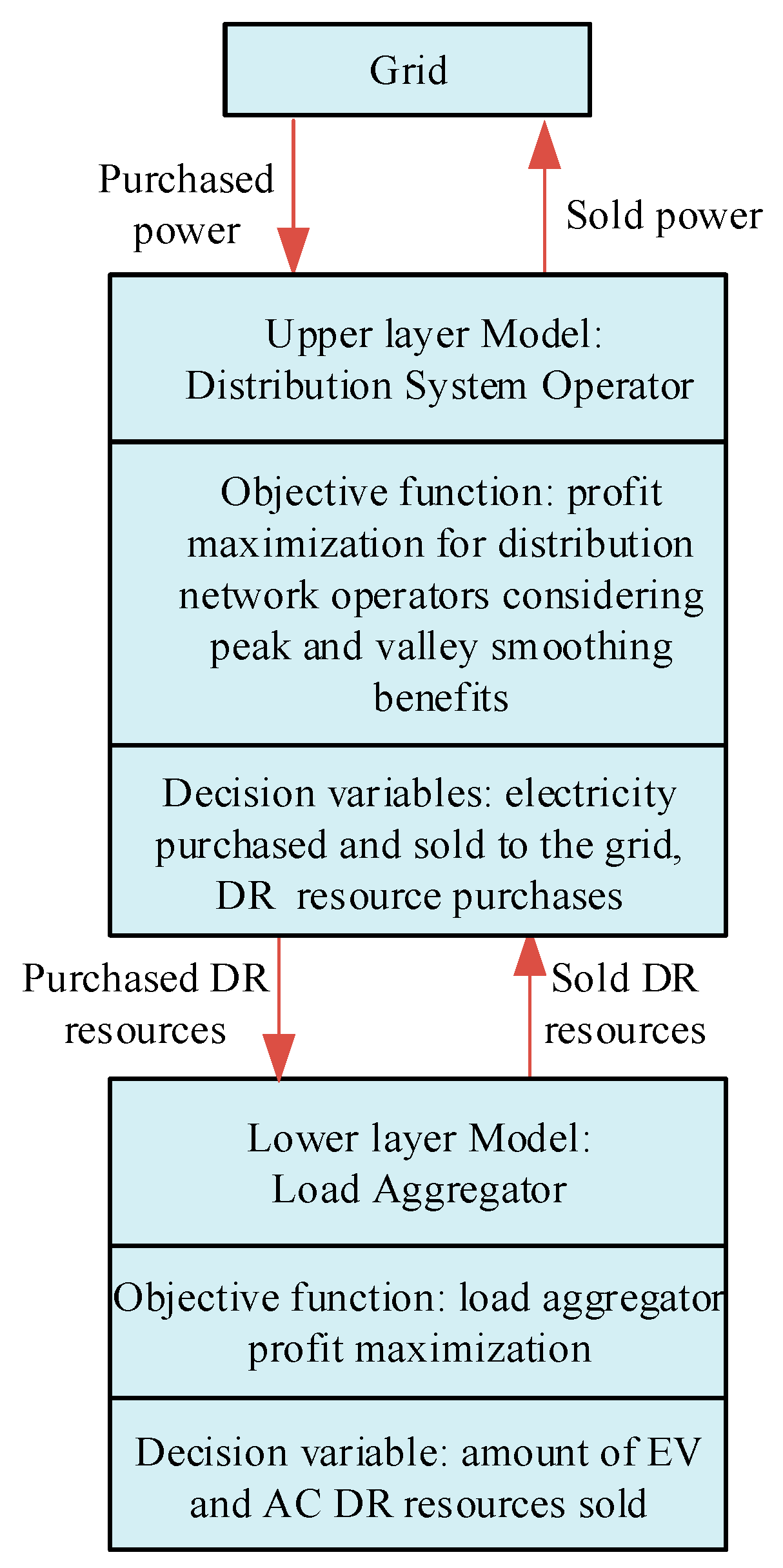
4. A Flexible Load Bilevel Optimization Model Considering Peak–Valley Smoothing Benefits

It is assumed that the wind and PV power sources under the jurisdiction of the DSO in the upper layer can be used to obtain the output curves based on day-ahead forecasts. The DSO, as the leader of the upper layer model, purchases the amount of response of the flexible loads in the station area from the LA, with the objective of maximizing the revenue of the DSO; the LA, as the follower, has the objective function of maximizing the profit gained from the participation of the flexible loads in the demand-side response through the dispatch of the flexible loads. The gains of both the upper and lower layers of the proposed two-tier optimization model are related to the amount of demand response resources, i.e., the objective values of the upper and lower layers interact with each other. The resulting two-layer model architecture is shown in Figure 3.

4.1. Upper-Layer Model Objective Functions and Constraints

The objective function of the upper-level model is to maximize the daily net profit of the DSO considering the peak and valley smoothing benefits, as shown in Equation (10). The net profit of the DSO is equal to the DSO’s revenue from electricity sales minus the expenditures for purchasing the amount of DR resources from the LA, the operation and maintenance costs of the wind and PV, the peak and valley smoothing benefits, the cost of purchasing electricity from the grid and the revenue from the sale of electricity. The decision variables are the number of EVs transferred, the amount of electricity purchased and sold to the grid, the amount of air conditioning curtailment, the peak-to-valley difference, and the load fluctuation.

The mathematical model of the upper-level optimization objective is:

$$D.S_{upper}=\max {\displaystyle \sum _{t=1}^T{R}_{sell}^t-R_{grid}^t-f_{drbuy}^t-f_{ope}^t}+f_{avg}^t$$

(12)

where $R_{sell}^t$ is the revenue from electricity sales to customers; $f_{drbuy}^t$ is the expenditure on purchasing flexible load demand response resources; $f_{ope}^t$ is the operation and maintenance cost of wind power and PV; $R_{grid}^t$ is the revenue from the purchase and sale of electricity from the grid; and $f_{avg}^t$ is the peak and valley smoothing benefit.

$$R_{sell}^t=P_{sell}^t{c}_{cell}^t$$

(13)

where $P_{sell}^t$ is the amount of electricity sold after the demand response, and $c_{sell}^t$ is the tariff of electricity sold by the distribution network operator to the customer:

$$R_{grid}^t=P_{bgrid}^t{c}_{bgrid}^t-P_{sgrid}^t{c}_{sgrid}^t$$

(14)

where $P_{bgrid}^t$ is the amount of electricity purchased from the grid, $P_{sgrid}^t$ is the amount of electricity sold to the grid, $c_{bgrid}^t$ is the price of electricity purchased from the grid, and $c_{sgrid}^t$ is the price of electricity sold to the grid.

$$f_{drbuy}^t=\Delta P_{AC}^t{e}_{AC}^t+\Delta P_{EV}^t{e}_{ev}^t$$

(15)

where $\Delta P_{AC}^t$ is the air conditioning load demand response; $\Delta P_{EV}^t$ is the electric vehicle demand response; $e_{EV}^t$ is the DSO’s call-off compensation tariff for purchasing units of electric vehicle load response from the LA; and $e_{AC}^t$ is the DSO’s call-off compensation tariff for purchasing units of air conditioning load demand response from the LA.

$$f_{ope}^t=P_{wt}^t{c}_{wt}+P_{pv}^t{c}_{pv}$$

(16)

where $P_{wt}^t$ and $P_{pv}^t$ are the wind power and PV output power predicted on the previous day, respectively, and ${\mathrm{c}}_{wt}$, ${\mathrm{c}}_{pv}$ are the operation and maintenance costs of wind power and PV, respectively.

To avoid the “peak-on-peak” phenomenon in the demand-side response results, which jeopardizes the safe and stable operation of the power grid while taking into account the profits of the load aggregators and the distribution network operators, a joint model of peak–valley smoothing benefits is introduced [26]:

$$f_{avg}^t=w_1\cdot \left(1-\frac{f_1}{f_{1M}}\right)+w_2\left(1-\frac{f_2}{f_{2M}}\right)$$

(17)

$$\begin{array}{l}{f}_1=\max \left(P_{sell}^t\right)-\min \left(P_{sell}^t\right)\\ f_{1M}=\max (P_M)-\min \left(P_M\right)\end{array}$$

(18)

$$f_{2M}={\left(P_M-{\displaystyle \sum _{t=1}^T\frac{P_M}{T}}\right)}^2$$

(19)

$$f_2={\left(P_{sell}^t-{\displaystyle \sum _{t=1}^T\frac{P_{sell}^t}{T}}\right)}^2$$

(20)

where $f_{avg}^t$ is the peak–valley smoothing benefit function; $P_M$ is the load before the demand response; $P_{sell}^t$ is the load after the demand response; $f_1$ is the peak–valley difference after the demand response; $f_{1M}$ is the peak–valley difference before the demand response; $f_{2M}$ is the amount of load fluctuation before the demand response; and $f_2$ is the amount of load fluctuation after the demand response. $w_1,w_2$ are the benefit coefficients. The constraints of the upper-level model are as follows:

(1)

Power balance constraints

The sum of the wind and PV output power and the power purchased from the grid by the distribution grid operator should be equal to the sum of all the loads, i.e.,:

$$P_{wt}^t+P_{pv}^t+P_{bgrid}^t=P_{\mathrm{s}ell}^t+P_{sgrid}^t+P_{load}$$

(21)

(2)

Grid power purchase and sale constraints:

$$\begin{array}{l}0\le P_{bgrid}^t\le {\gamma }_1{P}_{bgrid}^{\max }\\ 0\le P_{sgrid}^t\le {\gamma }_2{P}_{sgrid}^{\max }\end{array}$$

(22)

$${\gamma }_1+{\gamma }_2=1$$

(23)

where $P_{bgrid}^{\max }$ is the maximum amount of power purchased and $P_{sgrid}^{\max }$ is the maximum amount of power sold. ${\gamma }_1$ and ${\gamma }_2$ are variables 0 and 1, respectively, and the grid can only purchase and sell electricity at each moment.

4.2. Lower-Level Model Objectives and Constraints

The LA acts as an intermediary between the DSO and the user side, and generates revenue by aggregating the amount of flexible load response resources to sell to the DSO. The objective function of the lower layer model is:

$$L{A}_{lower}=\max {\displaystyle \sum _{t=1}^T{f}_{drbuy}^t-}{\displaystyle \sum _{t=1}^T{f}_{dr}^t}$$

(24)

$${\displaystyle \sum _{t=1}^T{f}_{dr}^t}=\left(\Delta P_{AC.d}^t{c}_{AC}^t+\left(\Delta P_{EV,d}^t+\Delta P_{EV,u}^t\right)c_{EV}^t\right)$$

(25)

where $\Delta P_{EV.d}^t$ is the transfer out of EVs,  $\Delta P_{EV.d}^u$ is the transfer in of EVs, $\Delta C_{AC}^t$ is the compensation tariff for air conditioning, and $C_{EV}^t$ is the transfer tariff for EVs.

The EV load is treated as a transferable load, and the transfer does not exceed its upper and lower limits, i.e.,:

$$0\le \Delta P_{EV.u}^t\le P_{EV}^{lit,t}{\beta }_{b,t},\hspace{1em}\hspace{1em}\forall b,t:{\mu }_1^{b,t},{\mu }_2^{b,t}$$

(26)

$$0\le \Delta P_{EV,d}^t\le P_{EV}^{lit}{\alpha }_{\alpha ,t},\hspace{1em}\hspace{1em}{\forall }_{a,t}:{\mu }_3^{a,t},{\mu }_4^{a,t}$$

(27)

$${\displaystyle \sum _{a=1}^T{\alpha }_{a,t}+{\displaystyle \sum _{b=1}^T{\beta }_{b,t}}\le 1,\hspace{1em}\hspace{1em}\forall t:}{\mu }_5^t$$

(28)

$${\displaystyle \sum _{t=1}^T\Delta P_{EV,d}^t={\displaystyle \sum _{t=1}^T\Delta P_{EV,u}^t}}\hspace{1em}\hspace{1em}\forall t:{\delta }_1$$

(29)

where $P_{EV}^{lit,t}$ is the upper limit of EV transfer; ${\alpha }_{a,t}$ and ${\beta }_{b,t}$ are the EV transfer-in and transfer-out state variables, which are 0 and 1 variables, respectively; ${\mu }_1^{b,t},{\mu }_2^{b,t},{\mu }_3^{a,t},{\mu }_4^{a,t},{\mu }_5^t,{\delta }_1$ are the corresponding Lagrangian equation multiplier constraints and unequal multiplier constraints, respectively; and Equation (29) indicates that the transfer-out of EV loads is equal to that of the transfer-in.

Reductions in air conditioning satisfy the following constraints:

$$0\le \Delta P_{AC,d}^t\le P_{AC}^{lit,t}\hspace{1em}\hspace{1em}\forall t{\mu }_6^t,{\mu }_7^t$$

(30)

where ${\mu }_6^t,{\mu }_7^t$ is the Lagrange multiplier constraint associated with the air conditioning reduction, and $P_{AC}^{lit,t}$ is the upper limit of aggregated air conditioning that can be reduced to satisfy the user’s comfort at moment t.

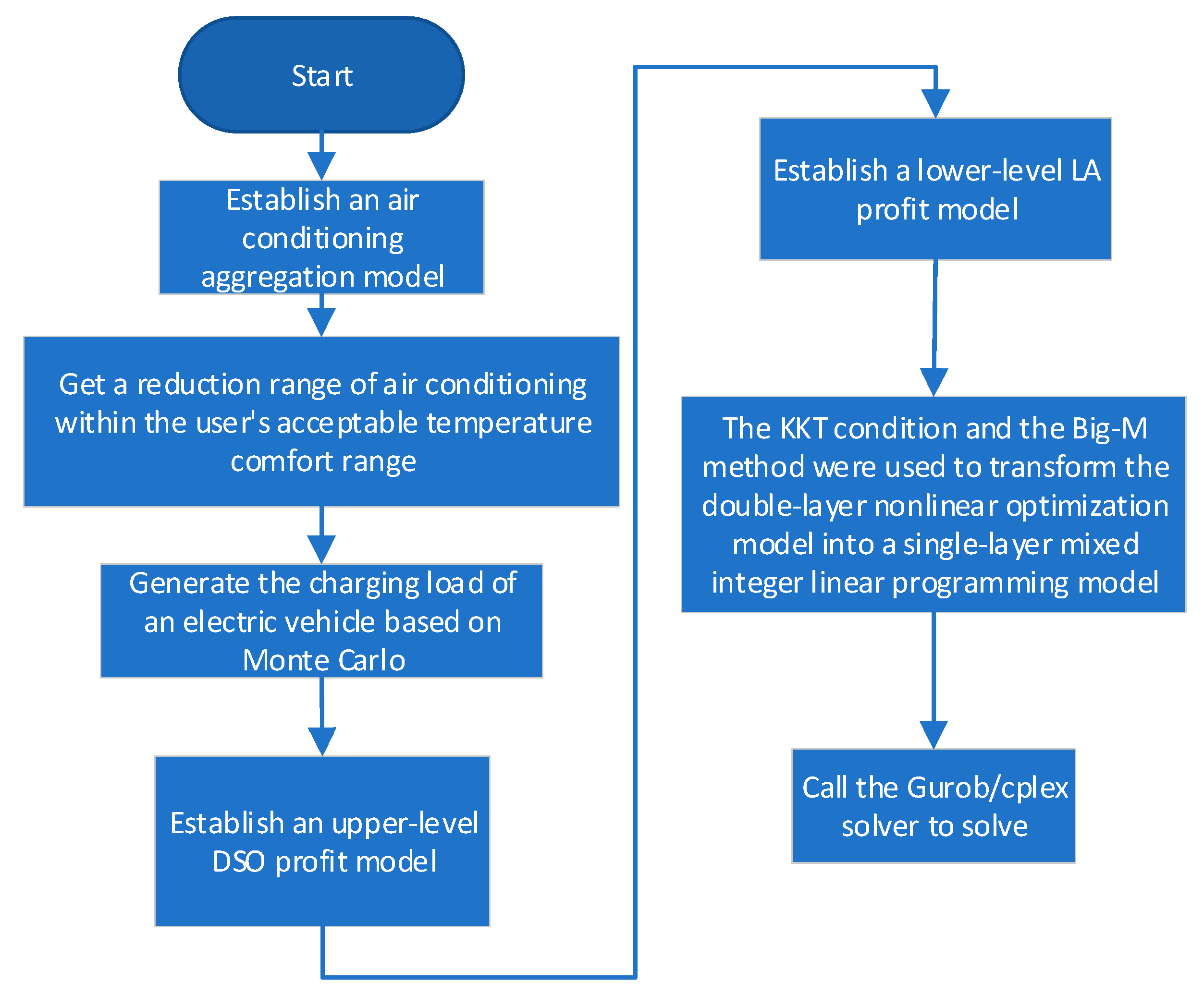
4.3. DLPO Model Solving

According to the two-tier model of this paper, the amount of demand response resources purchased by the upper tier affects the profit of the lower tier; thus, the upper and lower tiers are coupled. The solution method in this section is to transform the objective function and constraints of the lower-layer model into constraints of the upper-layer model using the KKT condition and then transform the single-layer nonlinear problem into a single-layer linear problem using the big-M method. The lower layer model is first utilized to construct the Lagrangian function:

$$\begin{array}{l}L\left(\Delta P_{EV,d}^t,\Delta P_{EV,p}^t,\Delta P_{AC,d}^t,\mu ,\delta \right)=\\ \Delta P_{AC}^t{e}_{AC}^t+\left(\Delta P_{EV,d}^t+\Delta P_{EV,u}^t\right)e_{EV}^t-\\ \left(\Delta P_{AC.d}^t{c}_{AC}^t+\left(\Delta P_{EV.d}^t+\Delta P_{EV,u}^t\right)c_{EV}^t\right)\\ +{\mu }_2^{b,t}\left({\beta }_{b,t}{P}_{EV}^{lit,t}-\Delta P_{EV,u}^t\right)+{\mu }_3^{a,t}\Delta P_{EV,d}^t\\ +{\mu }_4^{a,t}\left({\alpha }_{a,t}{P}_{EV}^{lit,t}-\Delta P_{EV.d}^t\right)++{\mu }_1^{b,t}\Delta P_{EV,u}^t\\ {\mu }_5^t\left(1-{\displaystyle \sum _{t=1}^T{\alpha }_{a,t}+{\displaystyle \sum _{t=1}^T{\beta }_{b,t}}}\right)+{\mu }_6^t\Delta P_{AC.d}^t+\\ {\mu }_7^t\left(P_{AC}^{lit,t}-\Delta P_{AC.d}^t\right)+{\delta }_1\left(\Delta P_{EV.d}^t-\Delta P_{EV,u}^t\right)\end{array}$$

(31)

Using the KKT condition again, we can obtain:

$$\frac{\partial L}{\partial \Delta P_{EV,d}^t}=e_{EV}^t-c_{EV}^t+{\mu }_3^{a,t}-u_4^{a,t}+{\delta }_t=0$$

(32)

$$\frac{\partial L}{\partial \Delta P_{EV,u}^t}=e_{EV}^t-c_{EV}^t+{\mu }_1^{b,t}-{\mu }_2^{b,t}-{\delta }_1=0$$

(33)

$$\frac{\partial L}{\partial \Delta P_{AC,d}^t}=e_{AC}^t-c_{AC}^t+{\mu }_6^t-{\mu }_7^t=0$$

(34)

$$0\le \Delta P_{EV,u}^t\perp {\mu }_1^{b,t}\ge 0$$

(35)

$$0\le \left({\beta }_{b,t}{P}_{EV}^{lit,t}-\Delta P_{EV,u}^t\right)\perp {\mu }_2^{b,t}\ge 0$$

(36)

$$0\le \Delta P_{EV,d}^t\perp {\mu }_3^{a,t}\ge 0$$

(37)

$$0\le \left({\alpha }_{a,t}{P}_{EV}^{lit,t}-\Delta P_{EV.d}^t\right)\perp {\mu }_4^{a,t}\ge 0$$

(38)

$$0\le \left(1-{\displaystyle \sum _{t=1}^T{\alpha }_{a,t}+{\displaystyle \sum _{t=1}^T{\beta }_{b,t}}}\right)\perp {\mu }_5^t\ge 0$$

(39)

$$0\le \Delta P_{AC.d}^t\perp {\mu }_6^t\ge 0$$

(40)

$$0\le \Delta P_{AC.d}^t\perp {\mu }_6^t\ge 0$$

(41)

$$0\le \left(P_{AC}^{lit,t}-\Delta P_{AC.d}^t\right)\perp {\mu }_7^t\ge 0$$

(42)

Equations (29)–(39) are complementary relaxation conditions, where $0\le a\perp b\ge 0$ denotes that $a\ge 0,b\ge 0$ and $ab=0$ are nonlinear problems, which need to be converted to linear constraints using the big-M method:

$$\{\begin{array}{l}0\le \Delta P_{EV,u}^t\le v_{1}M\\ 0\le {\mu }_1^{b,t}\le \left(1-v_1\right)M\end{array}$$

(43)

$$\{\begin{array}{l}0\le \left({\beta }_{b,t}{P}_{EV}^{lit,t}-\Delta P_{EV,u}^t\right)\le v_{2}M\\ 0\le {\mu }_2^{b,t}\le \left(1-v_2\right)M\end{array}$$

(44)

$$\{\begin{array}{l}0\le \Delta P_{EV,d}^t\le v_{3}M\\ 0\le {\mu }_3^{a,t}\le \left(1-v_3\right)M\end{array}$$

(45)

$$\begin{array}{l}\{\begin{array}{l}0\le \left({\alpha }_{a,t}{P}_{EV}^{lit,t}-\Delta P_{EV.d}^t\right)\le v_{4}M\\ 0\le {\mu }_4^{a,t}\le \left(1-v_4\right)M\end{array}\end{array}$$

(46)

$$\begin{array}{l}\{\begin{array}{l}0\le \left(1-{\displaystyle \sum _{t=1}^T{\alpha }_{a,t}+{\displaystyle \sum _{t=1}^T{\beta }_{b,t}}}\right)\le v_{5}M\\ 0\le {\mu }_5^t\le \left(1-v_5\right)M\end{array}\\ \end{array}$$

(47)

$$\{\begin{array}{l}0\le \Delta P_{AC.d}^t\le v_{6}M\\ 0\le {\mu }_6^t\le \left(1-v_6\right)M\end{array}$$

(48)

$$\begin{array}{l}\{\begin{array}{l}0\le \left(P_{AC}^{lit,t}-\Delta P_{AC.d}^t\right)\le v_{7}M\\ 0\le {\mu }_7^t\le \left(1-v_7\right)M\end{array}\end{array}$$

(49)

where $v_1,v_2,v_3,v_4,v_5,v_6,v_7$ are 0.1 variables, the objective function of this paper’s two-layer model after transformation by the KKT and Big-M methods is Equation (12), and the constraints are Equations (13)–(23) and (32)–(49). The flow chart of the two-layer optimization model proposed in this paper is as follows in Figure 4.

5. Calculation Analysis

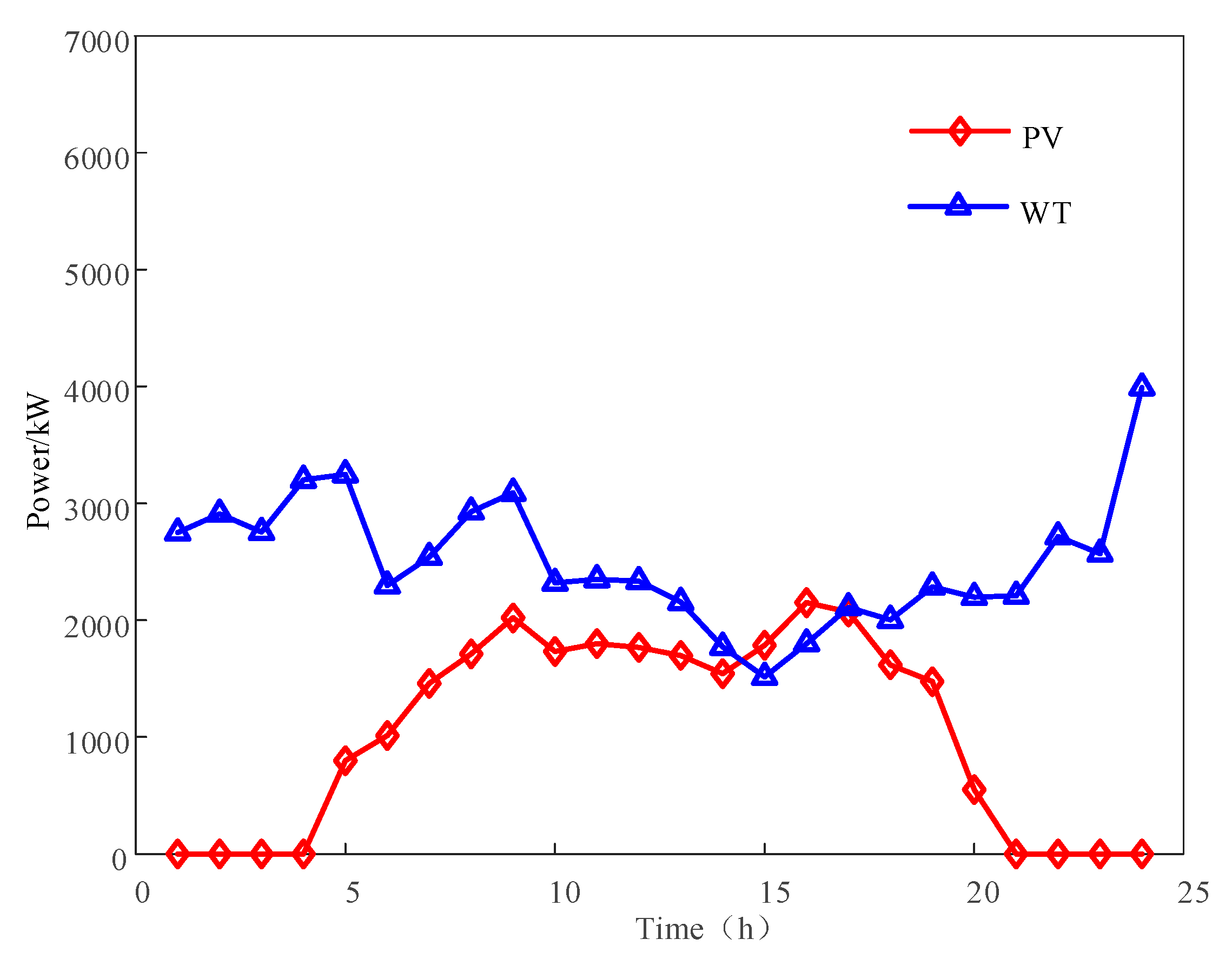
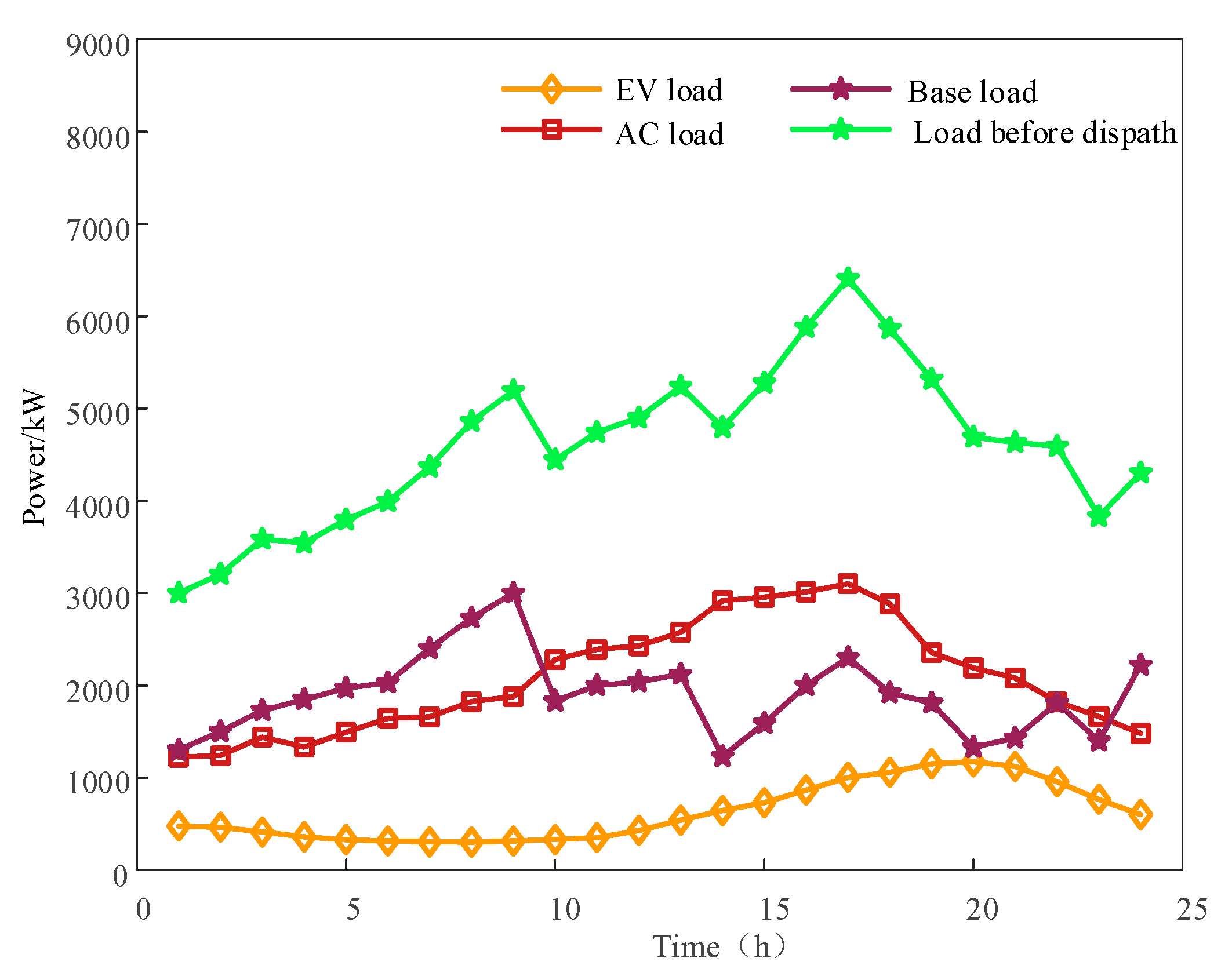
5.1. Scene Setting

The example selects typical daily load data in a southern region in summer, with a time scale of 1 h. Figure 5 shows the PV and WT output curves on a typical day, and WT and PV output modeling with reference to the literature [27]. Assuming that the initial set temperature of the air conditioning load of 1000 units in the region follows a random distribution in the interval [22 °C, 25 °C], the number of electric vehicles is 1200 and the electric vehicles need to be filled every time they are charged. According to Equations (1)–(5), the aggregated load curve of air conditioning from 1:00–24:00 can be obtained, and (6)–(11) can be obtained from the aggregated load curve of electric vehicles from 1:00–24:00. The load before dispatch is equal to the sum of the base load, air conditioning load, and EV load. As shown in Figure 6, it is assumed that the operation and maintenance costs of PVs and wind turbines are 0.02/(kW·h) and 0.01/(kW·h), respectively. The compensation tariff of the air conditioner is 0.1 Yuan/(kW·h), and the compensation tariff of the electric vehicle [16], is 0.2 Yuan/(kW·h);

Table 1. Electric vehicle parameters.

${\mathit{\mu }}_{\mathit{s}}$	${\mathit{\sigma }}_{\mathit{s}}$	${\mathit{\sigma }}_{\mathit{L}}$	${\mathit{\mu }}_{\mathit{L}}$
1.5–2.5	1.5–2.5	2.6–3	1000

shows the electric vehicle parameters,

Table 2. Air conditioning equipment parameters.

R	C	η	N
1.5–2.5 $\mathsf{\Omega }$	1.5–2.5 F	2.6–3	1000

shows the air conditioning parameters,

Table 3. Time-of-use tariff information.

Period	Specific Time Slots	Price/Yuan
Peak period	14:00—21:00	1.2
Bottom period	0:00—8:00	0.4
Smooth period	9:00–13:00 22:00—24:00	0.7

shows time-of-use tariff information; four scenarios are established as follows.

Scenario 1: Joint demand-side response of air-conditioning and electric vehicle loads considering peak-to-valley smoothing benefits.

Scenario 2: Joint demand-side response for air conditioning and electric vehicle loads without considering peak-to-valley smoothing benefits.

Scenario 3: Demand-side response for the air conditioning load without considering peak-to-valley smoothing benefits.

Scenario 4: Demand-side response for the EV load without considering peak-to-valley smoothing benefits.

In power systems, the peak-to-valley margin is often used to describe the smoothness of the load profile [24], and the smaller the peak-to-valley margin is, the smaller the impact on the grid, with the following expression:

$$P_{diff}=\frac{\max \left(P_{sell}^t\right)-\min \left(P_{sell}^t\right)}{\max \left(P_{sell}^t\right)}$$

(50)

where $P_{diff}$ is the peak-to-valley differential rate, $\max \left(P_{sell}^t\right)$ is the peak load, and $\min \left(P_{sell}^t\right)$ is the valley load.

The load volatility tends to reflect the degree of load dispersion, and the greater the load volatility is, the worse the electricity supply is. The resulting formula is obtained as follows:

$$R=\kappa \frac{\sqrt{\frac{1}{T}{\displaystyle \sum _{t=1}^T{\left(P_{sell}^t-{\displaystyle \sum _{t=1}^T\frac{P_{sell}^t}{T}}\right)}^2}}}{\frac{1}{T}{\displaystyle \sum _{t=1}^T{P}_{sell}^t}}$$

(51)

where $T$ is the time period; $\kappa$ = 1

5.2. Analysis of Simulation Results

The results of the demand side response for each scenario are as listed in

Table 4. Optimal scheduling results for each scenario of the system.

Classifications	1	2	3	4
DSO profit/Yuan	67,118	55,679	59,967	52,655
LA profit/Yuan	3474	2542	1273	1443
Peak-to-Valley Difference Rate	0.26	0.51	0.57	0.46
Load Fluctuation Rate	0.50	0.89	0.91	0.71

.

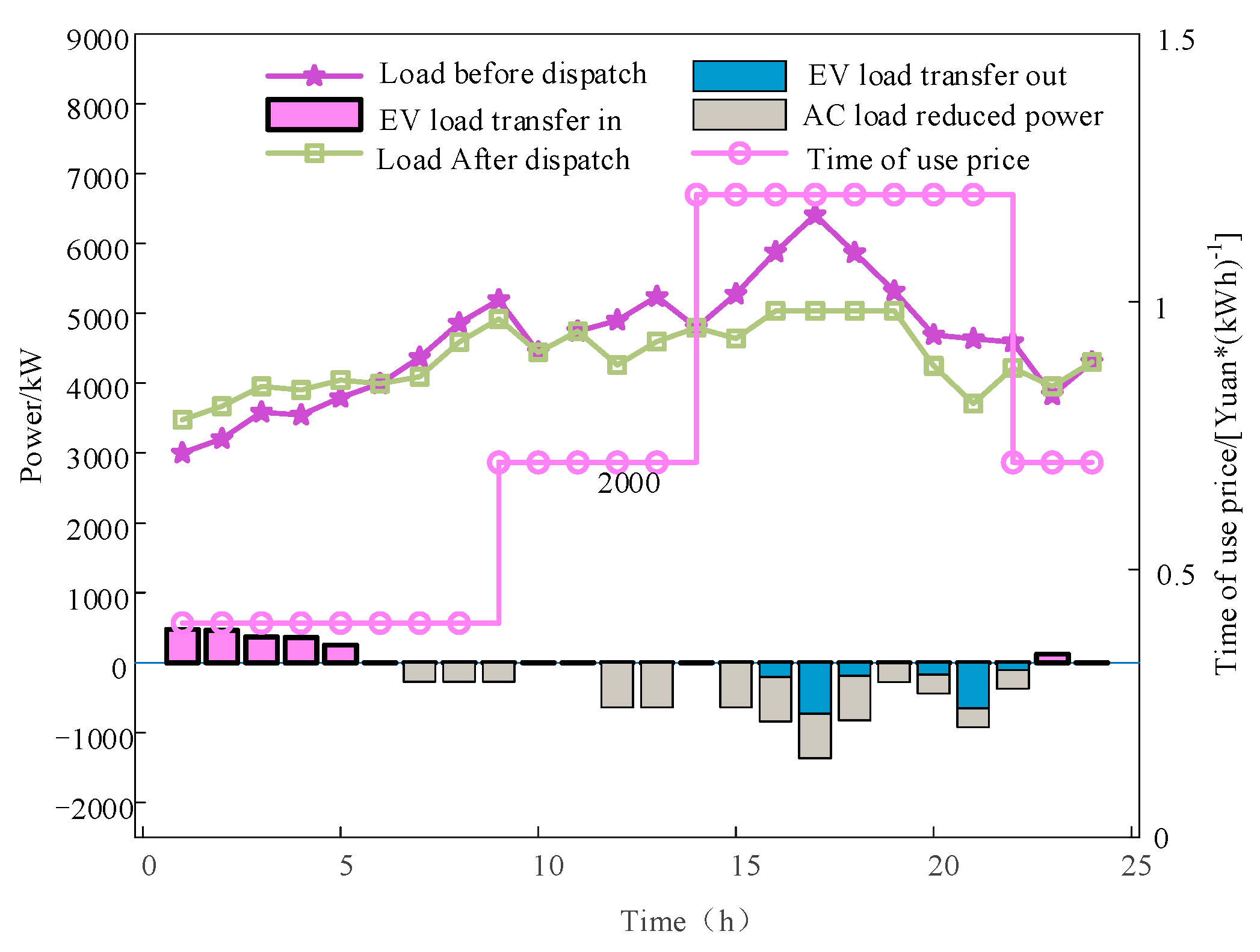
5.2.1. Scenario 1 Demand Side Response Results Analysis

Figure 7 shows the load changes before and after the response of scenario 1. Scenario 1 considers peak and valley smoothing benefits. At 0:00–5:00, EV loads are transferred, and EV loads are connected to the grid to start charging; thus, the load increases in this time period, and the valley load of the system, increases. In the 7:00–9:00 and 12:00–24:00 time periods, the air conditioning load participates in the demand response, the air conditioning load shows curtailment, the set temperature of the air conditioner increases, and the aggregated power of the air conditioner decreases. This is because the output of PV and wind turbines is not enough to meet the electricity needs of users in this time period, and the compensation price given by the DSO to the LA EV and air conditioner is higher in this time period. The LA can obtain a larger profit, and the peak load also decreases after dispatching.

The electric power supply and demand balance relationship for Scenario 1 is shown in Figure 8. The electric power balance relationship diagram shows that the DSO mainly meets the users’ electricity demand through its own PV and fan output. At 0:00–4:00, 6:00–7:00, and 10:00–24:00, the new energy output is not enough to meet the users’ electricity needs. Although the air conditioner decreases, it is still in the peak time period of electricity consumption, so the DSO purchases electricity from the grid. At 5:00 and 8:00–9:00, the new energy output is higher than the air-conditioning load, the electric vehicle load, and the base load, and at this time, there is a surplus of electricity that the DSO sells to the grid to earn revenue from the sale of electricity.

Figure 9 shows the gain curves of DSO and LA at each moment after the response of scenario 1. Compared with Figure 5, the 0:00–5:00 EV loads are transferred in and DSO provides the LA compensation cost; 16:00–19:00 EV loads are transferred out and air-conditioning loads are curtailed; the response compensation tariffs of EV loads and air-conditioning loads are high in this time period; and LA can obtain high flexible load response revenue from DSO. Although the DSO provides the LA with a high response cost, the DSO still makes a large profit from selling electricity to the customer because this time period is the peak period of electricity consumption, and the DSO has the highest gain from 16:00–19:00, as shown in Figure 9.

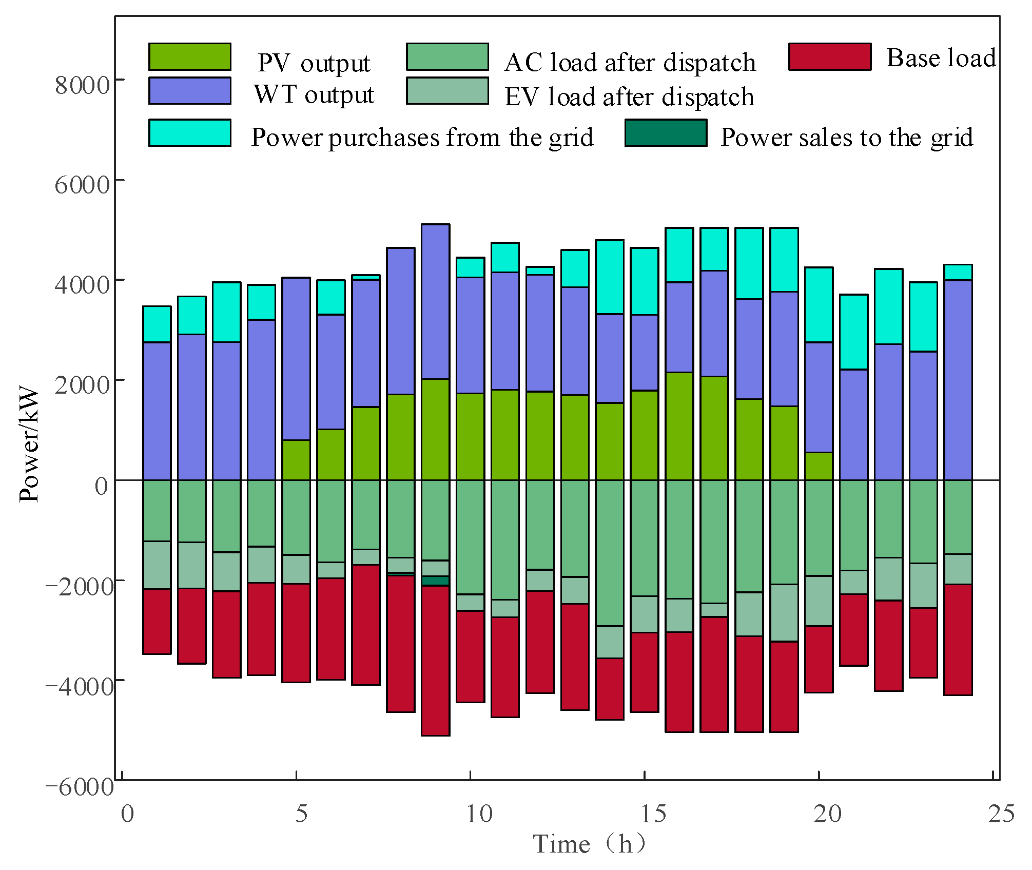
5.2.2. Comparison of the Results of the Joint Optimization of Electric Vehicles and Air Conditioning Loads

In scenario 4, only the EV loads participate in the demand response, at which time the air conditioning loads, as base loads, do not participate in the demand response. Scenario 3 is dispatched for air conditioning only, at which time EVs as the base load do not participate in the demand response. As shown in Table 4, the profits of DSO and LA in Scenario 2 are Yuan 55,679 and Yuan 2542, respectively; the profits of DSO and LA in Scenario 3 are Yuan 59,967 and Yuan 1273, respectively; and the daily profits of DSO and LA in Scenario 4 are Yuan 52,655 and Yuan 1443, respectively. The daily profit of DSO in Scenario 2 is slightly lower than that in Scenario 3 by Yuan 3025 than that in Scenario 4, and the daily profit of LA is higher than that in Scenario 3 and Scenario 4 by Yuan 1269 and Yuan 1099, respectively. In addition, the peak-to-valley difference rate and load fluctuation rate are also lower than those in Scenario 3 and are only slightly greater than those in Scenario 4, but substantially increase the overall profit of the distribution system. The joint scheduling of air conditioners and electric vehicles can optimize the peak and valley load profiles more effectively than the scheduling of air conditioners or electric vehicles alone, which not only compensates for the shortcomings of not being able to increase the valley load when only air conditioners are optimized, but also serves only as a curtailable load, and also compensates for the shortcomings of the response’s capability when only electric vehicles are involved in the demand response to reduce the peak load and increase the overall profitability of the power distribution system.

5.2.3. Comparison of Optimization Results Taking into Account Peak and Valley Smoothing Benefits

Scenario 1 considers peak–valley smoothing benefits in the optimization process. The greater the peak–valley difference and load fluctuation of the system are, the smaller the benefit of the DSO; thus, to ensure the maximum benefit of the DSO and LA, the system prefers to reduce the load peak–valley difference and reduce the load fluctuation. Therefore, at 0:00–5:00, the air conditioner is not cut, only by the electric vehicle load transfer, thus increasing the valley load. As shown in Table 4, the daily profit of the LA in Scenario 1 is Yuan 3474, that of Scenario 2 is Yuan 2542, and the daily profit of the LA in Scenario 1 is Yuan 932 higher than that in Scenario 2, which indicates that the consideration of the peak–valley smoothing benefit effectively exploits the response potential of flexible loads and improves the benefit of the LA. The peak-to-valley difference rate of Scenario 1 is 0.26, which is reduced by 0.25 compared with that of Scenario 2, and the load fluctuation rate is 0.5, which is reduced by 0.39 compared with that of Scenario 2, which indicates that the consideration of peak-to-valley smoothing benefits reduces the peak-to-valley difference and load fluctuation and ensures the safe and stable operation of the power system.

6. Conclusions

In this paper, a two-tier optimization model of flexible load demand-side response considering the benefits of peak and valley smoothing is constructed. The validity of the model is verified through a comparative analysis of four scenario examples. The following main conclusions are drawn:

(1)

The proposed two-layer optimization model considers the joint demand-side response of two flexible loads: air conditioning, and electric vehicles. The profit of the DSO and LA can be improved by the joint demand side response of flexible loads, compared with the single load demand side response.

(2)

The proposed two-tier optimization model introduces the benefit of peak–valley smoothing, which can effectively reduce the load peak–valley difference and load fluctuation compared with the demand-side response without considering peak–valley smoothing, and improve the profit of the LA and DSO while guaranteeing safe and stable power grid operation.

In our future work, we will take into account the uncertainty of wind power and photovoltaic output, and deeply explore the regulation potential of electric vehicles and air-conditioning loads, while taking into account the impact of seasonal factors, to help increase the level of new energy consumption and penetration.

References

1. Wang, C.; Gao, H.; Zhou, W.; Guo, M.; Liu, J. Dispatch optimization of high percentage new energy power system considering collinear demand response. Grid Technol. 2023, 10, 2023. [Google Scholar]
2. Aslam, W.; Andrianesis, P.; Caramanis, M. Optimal HVAC Energy and Regulation Reserve Scheduling in Power Markets. IEEE Trans. Sustain. Energy 2024, 15, 201–214. [Google Scholar] [CrossRef]
3. Chen, S.; Liu, C.-C. From demand response to transactive energy: State of the art. J. Mod. Power Syst. Clean Energy 2016, 5, 10–19. [Google Scholar] [CrossRef]
4. Kulkarni, A.; Brandes, G.; Rahman, A.; Paul, S. A Numerical Model to Evaluate the HVAC Power Demand of Electric Vehicles. IEEE Access 2022, 10, 96239–96248. [Google Scholar] [CrossRef]
5. Chen, Y.; Tian, H.; Liu, Y.; Chen, Z.; Li, C. Robust Optimal Allocation of Optical Storage and Charging in Highway Service Area Considering Demand Response of Electric Vehicles. Proc. CSEE 2023, 1–16. Available online: https://chn.oversea.cnki.net/kcms/detail/detail.aspx?filename=ZGDC20231115003&dbcode=CAPJ&dbname=CAPJLAST&uniplatform=NZKPT (accessed on 9 April 2024).
6. Afroz, Z.; Shafiullah, G.M.; Urmee, T.; Higgins, G. Modeling techniques used in building HVAC control systems: A review. Renew. Sustain. Energy Rev. 2018, 83, 64–84. [Google Scholar] [CrossRef]
7. Aste, N.; Manfren, M.; Marenzi, G. Building automation and control systems and performance optimization: A framework for analysis. Renew. Sustain. Energy Rev. 2017, 75, 313–330. [Google Scholar] [CrossRef]
8. Kong, X.; Sun, B.; Zhang, J.; Li, S.; Yang, Q. Power Retailer Air-Conditioning Load Aggregation Operation Control Method and Demand Response. IEEE Access 2020, 8, 112041–112056. [Google Scholar] [CrossRef]
9. Wang, Y.; Xiang, Y.; Hu, H.; Lao, K.W.; Tong, J.; Jiang, Y. Service-quality based pricing approach for charging electric vehicles in smart energy communities. J. Clean. Prod. 2023, 420, 138416. [Google Scholar] [CrossRef]
10. Hou, Y.; Zhao, L.; Jiang, H.; Ji, X.; Zhao, J. Two-Layer Control Framework and Aggregation Response Potential Evaluation of Air Conditioning Load Considering Multiple Factors. IEEE Access 2024, 12, 34435–34451. [Google Scholar] [CrossRef]
11. Zhang, Y.; Li, N.; Ding, H.; Lu, M.; Tang, D.; Wang, Q. Air conditioning load aggregation scheduling strategy based on users’ differentiated thermal comfort. Power Eng. Technol. 2023, 42, 133–140. [Google Scholar]
12. Li, Z.; Wu, L.; Xu, Y.; Zheng, X. Stochastic-Weighted Robust Optimization Based Bilayer Operation of a Multi-Energy Building Microgrid Considering Practical Thermal Loads and Battery Degradation. IEEE Trans. Sustain. Energy 2022, 13, 668–682. [Google Scholar] [CrossRef]
13. Shang, Y.; Li, S. FedPT-V2G: Security enhanced federated transformer learning for real-time V2G dispatch with non-IID data. Appl. Energy 2024, 358, 122626. [Google Scholar] [CrossRef]
14. Shen, X.; Li, J.; Yin, Y.; Tang, J.; Qian, B.; Lin, X.; Wang, Z. Multi-objective optimal scheduling considering low-carbon operation of air conditioner load with dynamic carbon emission factors. Front. Energy Res. 2024, 12, 1360573. [Google Scholar] [CrossRef]
15. Li, Q.; Zhao, Y.; Yang, Y.; Zhang, L.; Ju, C. Demand-Response-Oriented Load Aggregation Scheduling Optimization Strategy for Inverter Air Conditioner. Energies 2022, 16, 337. [Google Scholar] [CrossRef]
16. Wang, Q.; Huang, C.; Wang, C.; Li, K.; Xie, N. Joint optimization of bidding and pricing strategy for electric vehicle aggregator considering multi-agent interactions. Appl. Energy 2024, 360, 122810. [Google Scholar] [CrossRef]
17. Xin, S.; Li, J.; Yin, Y.; Tang, J.; Lin, X.; Qian, B. Bi-level optimal dispatching of distribution network considering friendly interaction with electric vehicle aggregators. Front. Energy Res. 2023, 11, 1338807. [Google Scholar] [CrossRef]
18. Joo, S.; Lee, D.; Kim, M.; Lee, T.; Choi, S.; Kim, S.; Lee, J.; Kim, J.; Lim, Y.; Lee, J. Multi-Agent Reinforcement Learning Based Actuator Control for EV HVAC Systems. IEEE Access 2023, 11, 7574–7587. [Google Scholar] [CrossRef]
19. Dadashi, M.; Haghifam, S.; Zare, K.; Haghifam, M.R.; Abapour, M. Short-term scheduling of electricity retailers in the presence of Demand Response Aggregators: A two-stage stochastic Bi-Level programming approach. Energy 2020, 205, 117926. [Google Scholar] [CrossRef]
20. Tavakoli, M.; Shokridehaki, F.; Marzband, M.; Godina, R.; Pouresmaeil, R. A two stage hierarchical control approach for the optimal energy management in commercial building microgrids based on local wind power and PEVs. Sustain. Cities Soc. 2018, 41, 332–340. [Google Scholar] [CrossRef]
21. Wang, X.; Li, F.; Dong, J.; Olama, M.M.; Zhang, Q.; Shi, Q.; Park, B.; Kuruganti, T. Tri-level Scheduling Model Considering Residential Demand Flexibility of Aggregated HVACs and EVs under Distribution LMP. In Proceedings of the 2022 IEEE Power & Energy Society General Meeting (PESGM), Denver, CO, USA, 17–21 July 2022. [Google Scholar]
22. Hou, H.; Xu, T.; Xiao, Z.F.; Deng, X.T.; Liu, P.; Xue, M. Integrated Optimal Scheduling of Power Generation and Consumption Considering Adjustable Load. Power Syst. Technol. 2020, 44, 4294–4304. [Google Scholar]
23. Cheng, L.-M.; Bao, Y.-Q. A Day-Ahead Scheduling of Large-Scale Thermostatically Controlled Loads Model Considering Second-Order Equivalent Thermal Parameters Model. IEEE Access 2020, 8, 102321–102334. [Google Scholar] [CrossRef]
24. Yang, Z.; Ding, X.; Lu, X.; Zhang, W.; Li, X.; Jing, J.; Gao, C. Load Modeling and Operation Control of Inverter Air Conditioner for Demand Response. Power Syst. Prot. Control. 2021, 49, 132–140. [Google Scholar]
25. Jin, X.; Zhang, Y.; Li, M.; Dou, X.; Ruan, W.; Duan, M. Differentiated assessment of residential air conditioning load regulation potential considering thermal comfort. Power Syst. Autom. 2024, 48, 50–58. [Google Scholar]
26. Shi, R.; Yang, H.; Ma, Y.; Wang, J.; Zhang, D. Demand response considering peak-to-valley smoothing benefits… Joint Optimization Strategy for Scheduling of Pool Energy Storage System. Electr. Power Autom. Equip. 2023, 43, 49–55. [Google Scholar]
27. Liu, Z.; Liu, Y.; Wang, X.; Qu, G. Operation Schedule Optimization of Energy Storage and Electric Vehicles in a Distribution Network with Renewable Energy Sources. Proc. CSEE 2022, 42, 1813–1826. [Google Scholar]
Figure 1. Flexible Load Demand Side Response Architecture.
Sustainability 16 03207 g001
Figure 2. Monte Carlo-based EV charging load generation.
Sustainability 16 03207 g002
Figure 3. Two-layer model architecture.
Sustainability 16 03207 g003
Figure 4. Model solving process.
Sustainability 16 03207 g004
Figure 5. Wind and PV output forecasts.
Sustainability 16 03207 g005
Figure 6. Load profile before the demand response.
Sustainability 16 03207 g006
Figure 7. Comparison of the load before and after the response in Scenario 1.
Sustainability 16 03207 g007
Figure 8. Power supply and demand equilibrium in Scenario 1.
Sustainability 16 03207 g008
Figure 9. Post-response DSO and LA gains at each time point.
Sustainability 16 03207 g009