Temporal Variations in Urban Air Pollution during a 2021 Field Campaign: A Case Study of Ethylene, Benzene, Toluene, and Ozone Levels in Southern Romania

Abstract

This study focused on quantifying the gas concentrations of ethylene, benzene, toluene, and ozone within an urban area in the southern region of Romania. The gas sampling campaign, conducted between March and August 2021, took place in three different locations from the point of view of the architectural structure, and the sampling height was 1.5 m. Sampling occurred on weekdays (Monday through Friday) during daylight hours, with subsequent concentration analysis employing descriptive statistics, diurnal cycles, and seasonal assessments. A highly sensitive and selective detector, employing laser photoacoustic spectroscopy, was utilized to monitor pollutants. The average concentrations (±Standard Deviation) were determined as follows: ethylene at 116.82 ± 82.37 parts per billion (ppb), benzene at 1.13 ± 0.32 ppb, toluene at 5.48 ± 3.27 ppb, and ozone at 154.75 ± 68.02 ppb, with peak levels observed during the summer months. Diurnal patterns were observable for ethylene, benzene, and toluene, exhibiting higher concentrations during the early hours of the day followed by a decrease towards the evening. In contrast, ozone concentrations peaked in the evening compared to the early part of the day. Thus, perceptible effects were demonstrated on gas concentrations as a result of the influence of meteorological variables. Moreover, the high toluene/benzene ratio indicated traffic and industrial emissions as primary sources of these pollutants. Of the four gases monitored, benzene and ozone exceeded regulatory limits, particularly during the summer season, highlighting concerns regarding air quality in the studied urban environment.

1. Introduction

Due to urbanization, human health and ecosystems are threatened by air pollution [1]. Despite the measures imposed by the European Environment Agency (EEA), air quality remains an important problem, and the concentrations of air pollutants continue to be very high [1,2]. An essential group of pollutants that requires particular consideration consists of volatile organic compounds (VOCs), compounds that can be involved in the generation of secondary pollutants like ozone (O₃) or secondary organic aerosol (SOA) [3,4]. VOCs encompass a diverse array of chemical substances [5,6], with specific emphasis placed on benzene, toluene, and ethylene. It is imperative to address this notable category of pollutants because of its contribution to the production of secondary pollutants like O₃ [3,4]. VOCs include a wide variety of chemical substances [5,6]; among them, special attention has been paid to benzene, toluene, and ethylene. Benzene (C₆H₆) is a compound found in various fuels, showing very low solubility in water and high volatility. It is also ranked in group 1 of substances with carcinogenic effects for humans by the International Agency for Research on Cancer (IARC) [7]. Toluene (C₇H₈) is a VOC present in crude oil and petroleum. Additionally, it is released into the atmosphere through the combustion of biomass [8]. Once in the atmosphere, its presence, influenced by meteorological conditions, contributes to the formation of smog along with other pollutants [9]. Ethylene (C2H4) is an organic compound recognized as a greenhouse gas released from plastic [10]. Royer et al. highlight that the level of ethylene in the ambient air is a concern, especially given the predictions that plastic production will double in the next 20 years [11]; currently, total global plastic production is approximately 8300 × 10⁶ Mt. [12,13]. Ethylene is considered a gas with a greenhouse effect, and in the atmosphere, under certain meteorological conditions, the ethylene molecule becomes a precursor of ozone in the troposphere [14,15,16].

In the atmosphere, pollutant gases can remain for long periods, and their elimination can be effected by their absorption by vegetation or as a result of chemical reactions with other gaseous compounds, reactions influenced by weather conditions [17]. These meteorological conditions favor the reaction between hydroxyl radicals, nitrogen oxides, and VOCs to form ozone [18]. Ground-level ozone is an aggressive pollutant both for ecosystems and for heating [19]. In the case of humans, once inhaled, it causes inflammation in the lungs and bronchi, and in those with cardiovascular and respiratory problems, a large amount of O₃ in the air can lead to aggravation of the disease and even death [16]. Despite the toxicity of these gases in the atmosphere, these pollutants are poorly monitored in Romania [20,21]. The composition of the atmosphere comprises various gases at different concentrations, which are influenced both by their sources and by meteorological conditions. To distinguish the different gas species, a detector with high selectivity and sensitivity is required. Laser photoacoustic spectroscopy (LPAS) is emerging as a technology capable of providing these essential features [22,23,24]. LPAS offers high sensitivity and selectivity, allowing the measurement of multiple gases over a wide dynamic range. It operates in the 3 to 12 μm spectral region, with very high parts per billion (ppb) detection sensitivity and response times of less than 1 s [22,23,24,25,26,27]. With this technique, to achieve specificity, the target molecules must exhibit a distinctive molecular fingerprint within the emission spectral range of the laser source [24]. Ethylene, benzene, toluene, and ozone molecules demonstrate absorption within the wavelength range of the laser source.

In this study, we explored soil-level VOCs such as ethylene, benzene, toluene, and ozone. The concentrations of these gases were in the order of ppb and were analyzed using a detector based on LPAS. The monitoring campaign took place in one of Romania’s most polluted regions, covering three distinct locations with varying architectural and environmental characteristics—within the city, in a forest, and an industrial area. Measurements were taken at a height of 1.5 m above the ground during the period from March to August 2021, encompassing both spring and summer seasons. This study aimed to determine gas concentrations, analyze their spatial distribution, assess the impact of meteorological variables, and sources, and investigate seasonal and diurnal variations.

2. Materials and Methods

2.1. Sampling Site

The atmospheric pollutant monitoring campaign was conducted in Magurele city, Romania (44°20′58″ N, 26°01′47″ E, altitude: 93 m), in the period March to August 2021, encompassing both spring and summer seasons. Romania, located in southeastern Europe, features a transitional temperate-continental climate [28]. Air sampling was conducted at three distinct locations within the city, each with unique architectural characteristics: P1: situated within the city amidst residential buildings and near an elementary school and a kindergarten. P2: positioned within a forest predominantly composed of oak (Quercus robur) and black locust (Robinia pseudoacacia). This location is encircled by two heavily trafficked roads, including the capital city beltway. P3: situated in an industrial area characterized by a lack of greenery.

Ambient air samples were collected at a height of 1.5 m above the ground using specialized containers/bags (750 mL aluminum-coated bags from Quintron), capable of retaining samples for up to 6 h. Passive sampling involves the collection of gas or vapor pollutants from the atmosphere without the need for active air movement; instead, sampling relies on physical processes such as diffusion. Sampling was conducted exclusively on weekdays, Monday through Friday, between 8:30 a.m. and 8:30 p.m. Each location underwent the collection of a total of six samples: three during the morning period (8:30 to 11:30 a.m.) and an additional three during the evening period (5:30 to 8:30 p.m.). This sampling strategy was designed to provide a comprehensive understanding of environmental conditions at different times of the day, enabling a thorough analysis of variations in trace gases or other relevant parameters throughout the day. The two sampling timeframes were essential for capturing potential diurnal fluctuations, ensuring a robust understanding of the environmental characteristics at each specific location. The results presented in this study are part of the same monitoring campaign for other pollutants, as reported elsewhere [22,29].

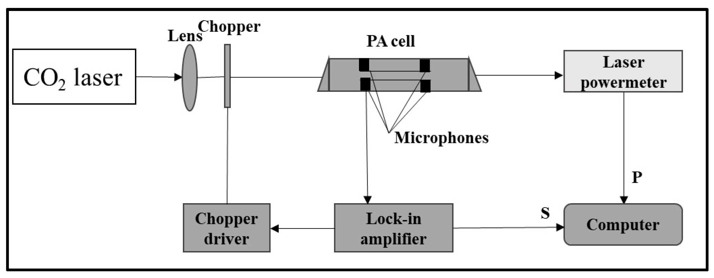
2.2. Laser Photoacoustic Spectroscopy Method and Passive Air Sampling

Gaseous pollutant concentrations in the ambient air were determined using a multicomponent detector, with high sensitivity and selectivity, based on laser photoacoustic spectroscopy. The photoacoustic effect is realized when the target molecules have a high absorption capacity of the radiation emitted by the laser source. Therefore, the molecules absorb the energy from the laser radiation and subsequently release it as heat. This process leads to a rise in pressure within a confined space, resulting in the generation of acoustic waves that can be detected by sensitive microphones [30,31].

Using the LPAS detector, we can realize a quantitative determination of the pollutant’s gas concentration. The photoacoustic system used to determine the concentrations of ethylene, benzene, toluene, and ozone consists of a CO₂ laser, a photoacoustic cell, a data acquisition system, and a gas handling system [30,31] (see Figure 1). The CO₂ laser serves as a frequency-stabilized laser source emitting continuously in a range of 57 different lines spanning from 9.2 to 10.8 µm, divided into four branches: 9R, 9P, 10R, and 10P. The continuous-wave (cw), tunable CO₂ laser beam undergoes chopping, is then focused by a ZnSe lens, and subsequently introduced into the photoacoustic (PA) cell. As the laser beam traverses the PA cell, its power is quantified using a laser radiometer, specifically the Rk-5700 model from Laser Probe Inc., featuring a measuring head designated as RkT-30. The digital output from this measurement is integrated into the data acquisition interface module alongside the output from the lock-in amplifier. All experimental data are subsequently processed and stored using a computer. To modulate the light beam, a high-quality mechanical chopper was employed, specifically the DigiRad C-980 or C-995 models with a 30-slot aperture. This chopper is characterized by low vibration noise and variable speed capabilities ranging from 4 to 4000 Hz, operating at the resonant frequency of the cell set at 564 Hz. The acoustic waves generated are captured by strategically positioned microphones in the cell wall. These microphone signals are then directed to a lock-in amplifier synchronized with the modulation frequency. Acting as a versatile signal recovery and analysis tool, the lock-in amplifier excels in accurately measuring a single-frequency signal even amidst noise sources thousands of times its magnitude. It effectively filters out random noise, transients, incoherent discrete frequency interference, and harmonics of the measurement frequency. We utilized a dual-phase, digital lock-in amplifier, specifically the Stanford Research Systems model SR 830, renowned for its impressive specifications: full-scale sensitivity ranging from 2 nV to 1 V; input noise at 6 nV (rms)/Hz at 1 kHz; dynamic reserve exceeding 100 dB; a broad frequency range spanning from 1 mHz to 102 kHz; and flexible time constants ranging from 10 μs to 30 s (for reference frequencies > 200 Hz) or extending up to 30,000 s (for reference frequencies < 200 Hz). In a photoacoustic system (LPAS), the formula for the measured trace gas concentration is expressed as follows: c = V/αPLCSM, where [31]:

-

c [atm] represents the trace gas concentration;

-

V [V] denotes the PA signal (peak-to-peak value);

-

α [cm⁻¹atm⁻¹] is the gas absorption coefficient at a specified wavelength;

-

P_L [W] signifies the continuous-wave laser power (unchopped value; twice the measured average value);

-

S_M [V Pa] is the microphone responsivity.

In some cases, the PA cell responsivity R [VcmW⁻¹] is used instead of the cell constant, defined as R = CS_M (this is a calibration constant or the merit factor of the cell). When V = V_min (at Signal-to-Noise Ratio, SNR = 1), the minimum detectable concentration (c = c_min) of the trace gas is obtained through the formula:

$$c_{min}=\frac{V_{min}}{\alpha P_{L}R}$$

The primary limiting factors of the LPAS system are interference gases. Under normal atmospheric conditions, the cumulative nature of the photoacoustic signal presents challenges for detection in the low-concentration range (parts per billion, ppb), particularly in the presence of significant amounts of water vapor and carbon dioxide. To tackle this issue, we utilize a potassium hydroxide (KOH) based scrubber positioned between the sampling cell and the PA cell. This setup initiates a specific chemical reaction: KOH → K₂CO₃ and water. As a result, interference from water vapor and carbon dioxide is alleviated, allowing for an accurate measurement of gas concentrations without the influence of these interfering gases. Experimental findings suggest that approximately 120 cm³ of KOH pellets are needed in an enclosure for a 750 mL sampling bag to effectively remove CO₂ and water vapor from ambient air samples. Before entering the PA cell, the gas sample passes through a chamber containing 120 cm³ of KOH pellets, reducing the concentration of interference gases. To ensure the highest precision in monitoring gaseous pollutants in ambient air, the PA cell is meticulously cleaned before each measurement using nitrogen 6.0 of 99.9999% purity. Additionally, to maintain a clean system without impurities, the background signal must be less than 20 µV/W. All cleaning and gas evacuation processes in the photoacoustic system are executed by the gas handling system. After cleaning the entire system, the target gas concentration is determined. The four gases in the ambient air show maximum absorption on different lines in the CO₂ laser emission range and different absorption coefficients α (cm⁻¹atm⁻¹), as follows, ethylene on the 10P(14) laser line with α = 30.4 cm⁻¹atm⁻¹ [31], benzene on the 9P(30) [32] laser line with α = 2 cm⁻¹atm⁻¹ [33], toluene on the 9P(28) laser line with α = 0.67 cm⁻¹atm⁻¹ [34], and ozone on the 9P(14) laser line with α = 12.4 cm⁻¹atm⁻¹ [35]. The acoustic waves generated by the absorption of laser radiation by these gas molecules are captured using four microphones, each with a sensibility of 20 mV/Pa. These microphones are connected in series and positioned on the wall of the PA cell, specifically at the loop position of the first longitudinal mode where the maximum pressure amplitude occurs. To ensure accurate concentration values, the PA cell is calibrated. The calibration of the PA system is typically conducted using a reference gas. In our case, we calibrated the PA cell using the widely employed reference gas, ethylene (C₂H₄), for which absorption coefficients are precisely known at CO₂-laser wavelengths. Ethylene proves to be highly suitable for calibration due to its weak interaction with common cell surface materials. It is chemically inert, shares the same molecular weight as nitrogen, and lacks a permanent dipole moment, resulting in negligible adsorption on the cell walls. Moreover, the spectrum of ethylene within the CO₂-laser wavelength range is highly structured. Notably, it features a distinctive absorption peak at the 10P(14) laser transition located at 949.49 cm⁻¹, attributed to the proximity of the Q branch of the ν7 vibration of C₂H₄ centered at 948.7715 cm⁻¹. Throughout our investigations, we utilized a commercially prepared and certified mixture containing 0.96 ppm of C₂H₄ in pure nitrogen. For calibration purposes, we examined this reference mixture at a total pressure (p) of approximately 1013 mbar and a temperature (T) of around 23 °C, using the widely accepted value of the absorption coefficient of 30.4 cm⁻¹atm⁻¹ at the 10P(14) line of the CO₂ laser. Under these conditions, the PA cell is characterized by a quality factor (Q) of 16.1, a cell constant (C) of 4375 Pa·cm/W, and a responsivity (R) of 350 cmV/W, indicating its sensitivity to pressure variations at a resonance frequency of 564 Hz.

2.3. Ambient Meteorological Variables

The impact of weather conditions on atmospheric gas concentrations was assessed by monitoring various weather parameters (ambient temperature, pressure, humidity, wind speed, and direction) using a Eurochron WS1080 wireless weather station. The station’s sensors measure these variables and send the data to a central unit, where it is recorded and stored by the base station on a computer.

3. Results

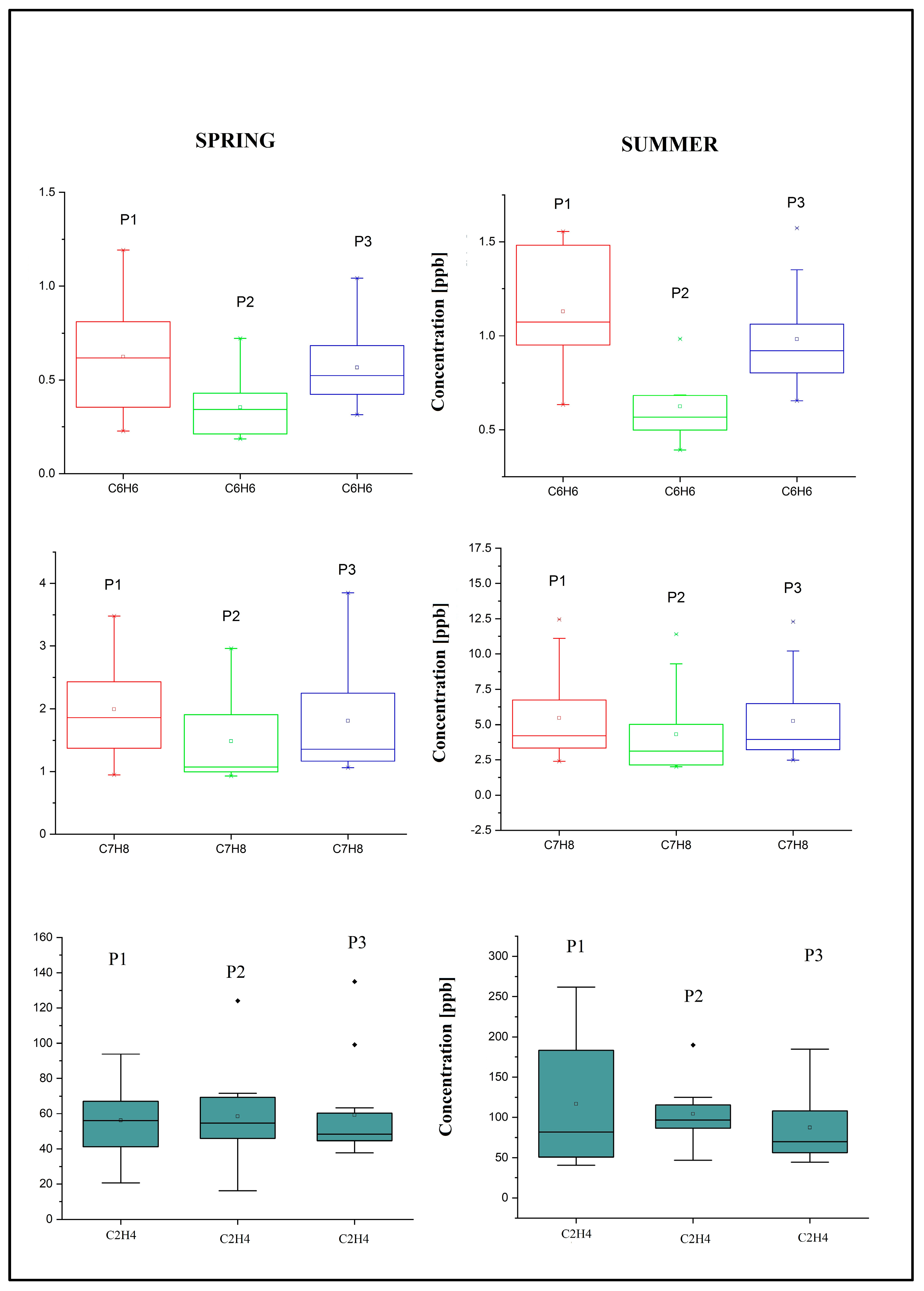
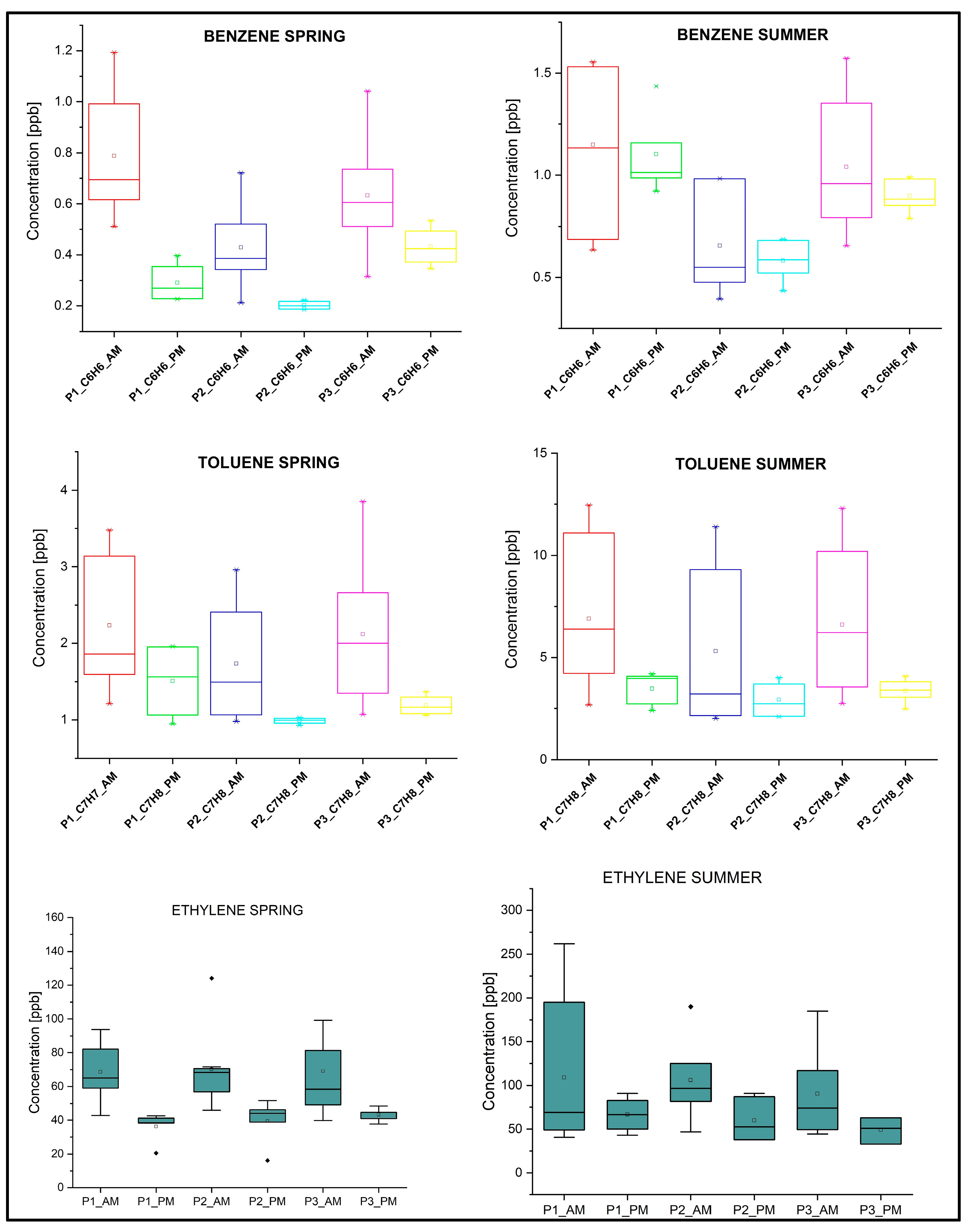
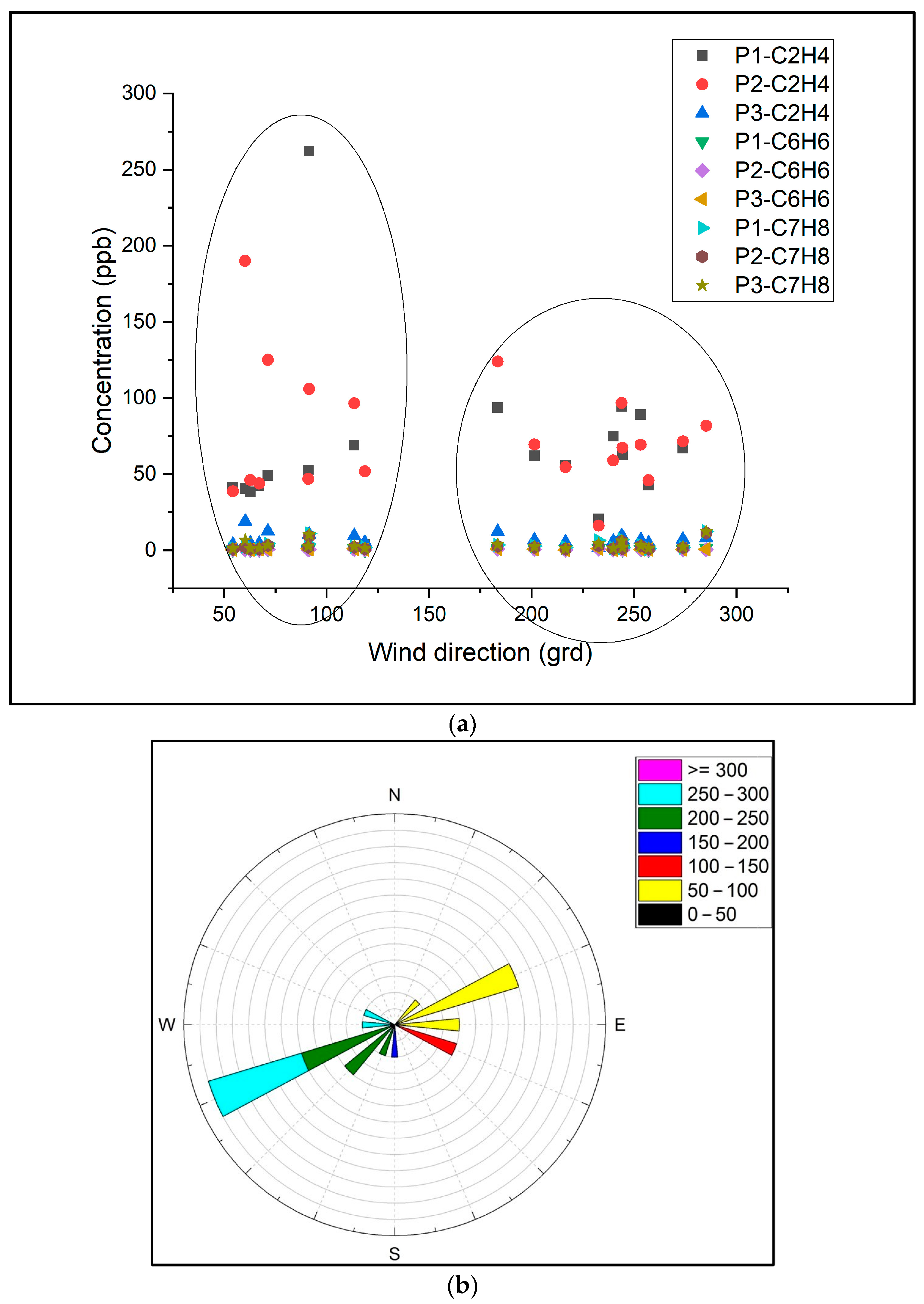
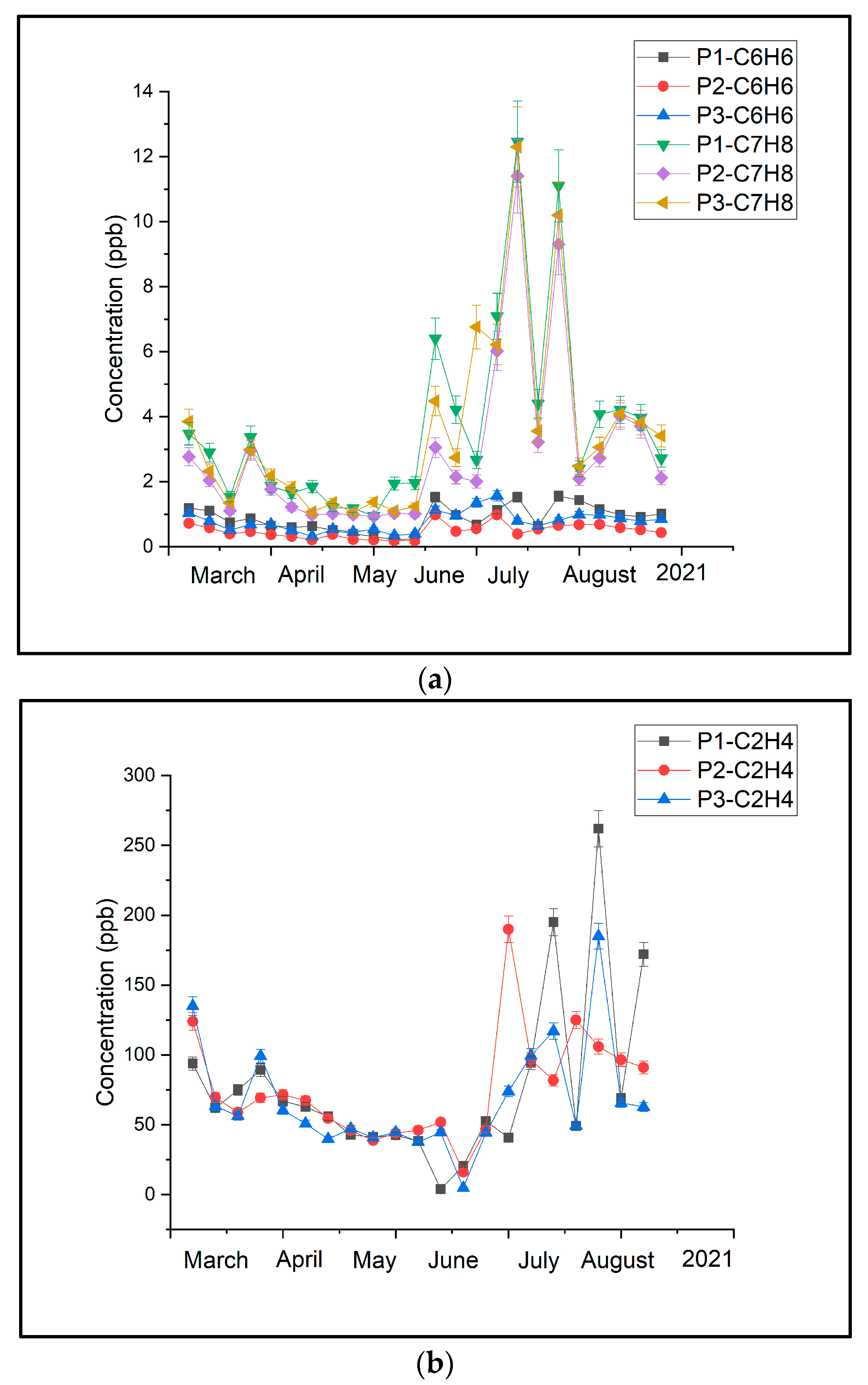
3.1. Atmospheric VOCs Measurements

The campaign to measure the four polluting gases in the atmosphere took place between March and August 2021 at three different points in a small town called Magurele, a town located in one of the most polluted areas in Romania [22,29]. The objective of this campaign was to use a detector based on LPAS to assess the concentration of certain gases in ambient air. Specifically, the focus was on three VOCs—ethylene, benzene, and toluene, as well as ozone. The primary aim was to identify potential patterns in concentration variations influenced by meteorological variables, including air temperature, wind speed, and direction. Additionally, the study objective was to analyze the impact of the architectural structure of the sampling sites and the sources of these pollutants. An additional objective was to investigate whether there exists a correlation between VOCs and ozone levels in the studied environment. To ascertain the concentrations of four gases—benzene, toluene, ethylene, and ozone—in the environment, gas samples were obtained from ambient air using a specialized aluminum bag on weekdays. These samples were subsequently analyzed in the laboratory employing the CO₂LPAS detector. Passive vapor monitoring or badges that collect air are used to measure ppb or ppm (parts-per-million) concentration levels. During our measurements, the maximum concentrations for benzene and toluene were determined in P1 point with 1.573 ppb and 12.46 ppb, and the minimum concentrations values were in P2 with 0.186 ppb and 1.01 ppb. The ethylene minimum concentration determined by our system was 3.85 ppb in the P2 point, and the highest concentration value was 262 ppb in the P1 point. The mean values ± standard deviation (SD) for the three VOCs measured in the spring and summer seasons in the three locations using the LPAS system are presented in

Table 1. Mean ± SD concentrations of ethylene, benzene, and toluene at points P1, P2, and P3 during spring and summer seasons.

VOCs	Spring Concentration ± SD ppb			Summer Concentration ± SD ppb
	P1	P2	P3	P1	P2	P3
ethylene	56.14 ± 21.49	58.34 ± 25.06	55.76 ± 31.61	116.86 ± 82.37	104.28 ± 41.17	87.23 ± 46.43
benzene	0.62 ± 0.32	0.35± 0.17	0.57± 0.21	1.13 ± 0.32	0.624 ± 0.19	0.98 ± 0.26
toluene	1.99 ± 0.84	1.49 ± 0.73	1.80 ± 0.88	5.48 ± 3.27	4.32 ± 3.07	5.26 ± 3.11

.

The temporal variation in ethylene, benzene, and toluene during the monitoring period with the mean concentration values is presented in Figure 2, and the seasonal behavior of the VOCs, the mean values of these gas concentrations during the monitoring months, March, April, and May in the spring season, and June, July, and August months for the summer are presented in Figure 3. In the presented figure, our focus was on examining the variance in pollutant concentrations in ambient air during the spring and summer seasons, as indicated by descriptive statistics. Notably, the concentrations of benzene, toluene, and ethylene consistently exhibit higher levels during the summer season across all three locations. Among these pollutants, benzene and toluene display their lowest concentrations at point P2, with the highest values recorded at point P1. Point P3 reveals higher concentrations for both benzene and toluene compared to those at P1, yet the overall average remains below that of P1. Ethylene exhibits a slightly distinct pattern in contrast to benzene and toluene, demonstrating elevated levels at point P2, surpassing even those at P3. However, the peak concentrations for ethylene are identified at point P1.

To conduct daily analyses and assess potential variations in concentrations during two distinct time intervals, air samples were collected and analyzed between 08:30 and 11:00 a.m. and 05:30 and 08:30 p.m. The diurnal patterns of benzene, toluene, and ethylene were examined using descriptive statistics, with the results presented in Figure 4. Elevated concentrations of ethylene, benzene, and toluene were observed in the morning, primarily attributed to human activities. In the evening, a temperature increase created favorable conditions for chemical reactions, subsequently leading to air layer dilution. This diurnal behavior of gaseous pollutants was further analyzed across both spring and summer seasons to determine if temperature does indeed influences gas concentration levels.

Furthermore, alongside the impact of temperature on ethylene, benzene, and toluene concentrations, we also tracked the influence of wind direction and speed. Figure 5 and Figure 6 illustrate the effects of wind speed and direction on monitoring gas concentrations.

An indicator for the source of atmospheric pollutants, such as traffic and/or industry is represented by the toluene/benzene (T/B) ratio [36], The values of the T/B ratio in the spring and summer seasons calculated in the monitoring sites P1, P2, and P3 are presented in

Table 2. The T/B ratio in the three measurement points on spring and summer seasons.

Location	Spring			Summer
	P1	P2	P3	P1	P2	P3
T/B ratio	3.21	4.26	3.16	4.85	6.92	5.37

.

The toluene/benzene (T/B) ratio is a commonly utilized indicator for distinguishing aromatic sources, widely recognized for its effectiveness in source identification. In regions significantly impacted by vehicle emissions, the T/B ratio typically ranges from 0.9 to 2.2 [37]. Instances of higher T/B ratios exceeding 8.8 are observed in solvent usage, while industrial processes often exhibit ratios ranging from 1.4 to 5.8 [38,39]. Studies focusing on emissions from combustion sources have reported T/B ratios below 0.6 in various combustion processes and raw materials [40]. Barletta et al. proposed that a T/B ratio higher than 5.0 is associated with industrial solvent usage, while a ratio of approximately 2.0 indicates traffic emissions [41]. According to the measurements presented in Table 2, our study reveals T/B ratios of approximately 3 and 4 in the spring and exceeding 5 in the summer. This suggests that the atmospheric presence of benzene and toluene in the measurement areas is attributed to both traffic and industrial emissions [42,43].

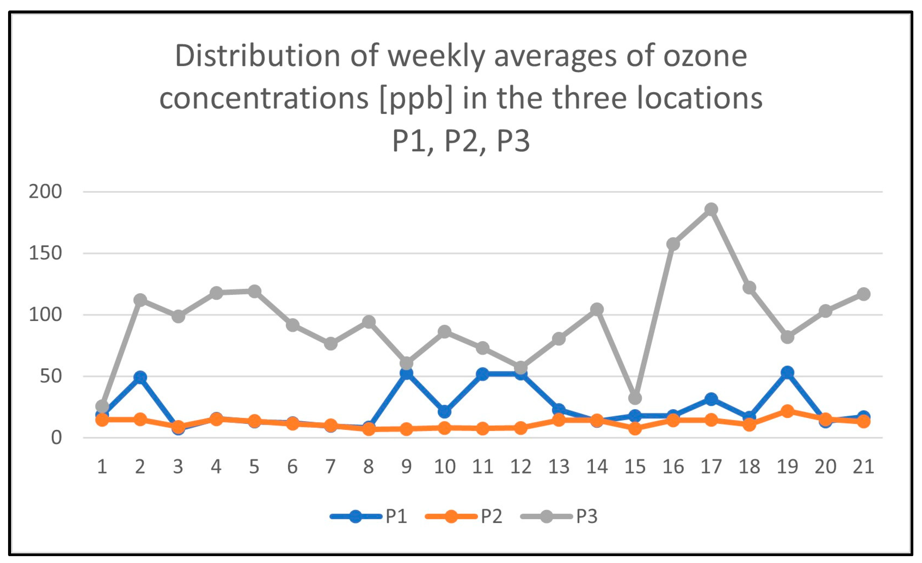
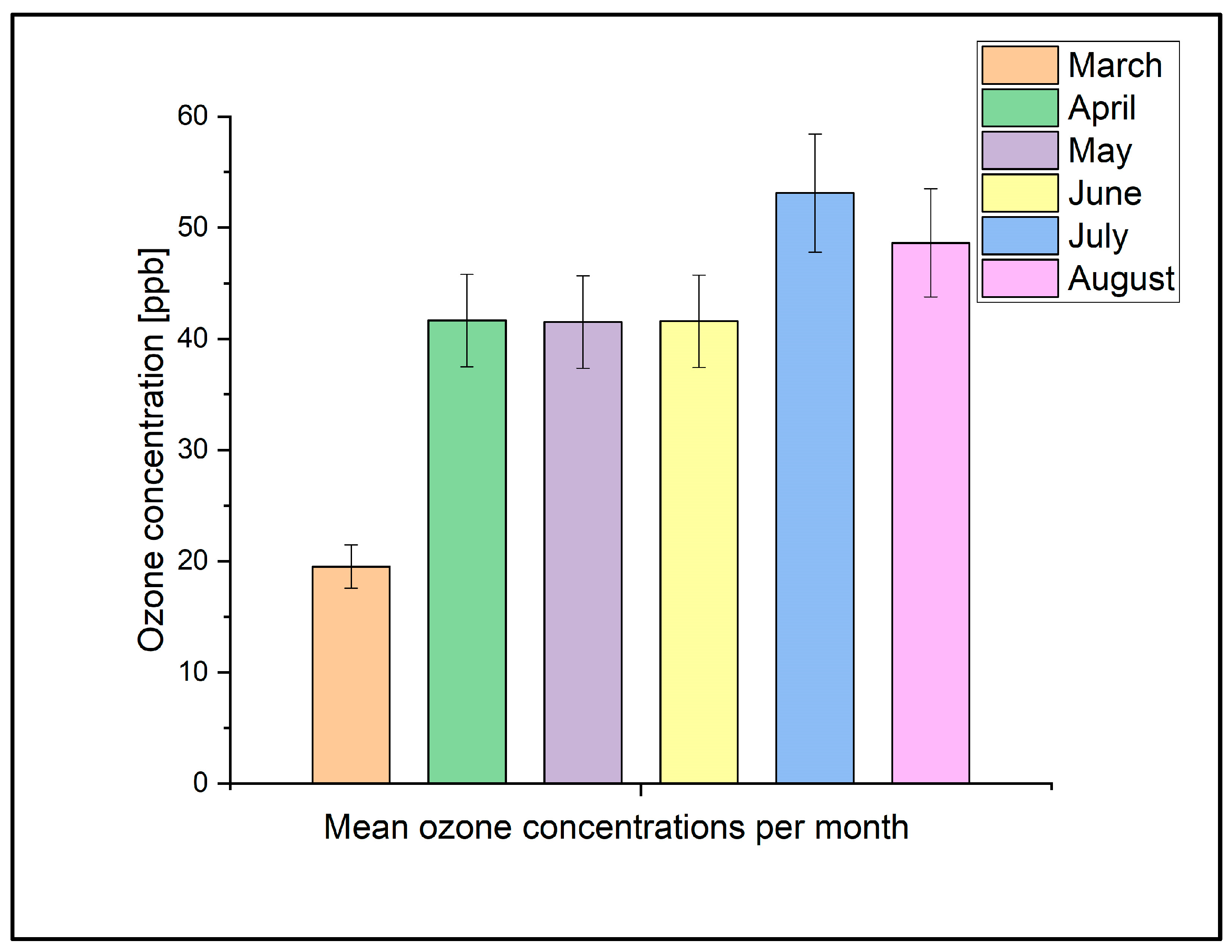
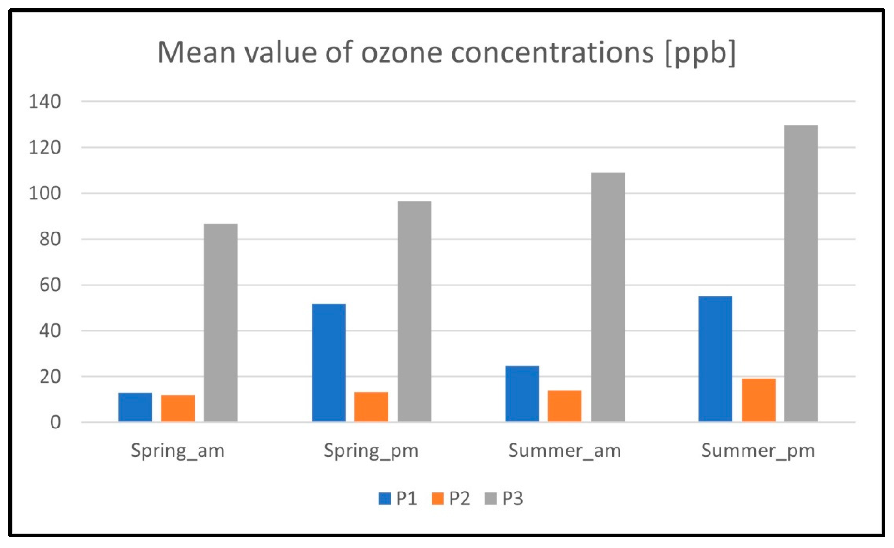
3.2. Atmospheric Ozone Measurements

Ozone gas is very harmful to humans and the environment, and the levels of this pollutant were determined using a PA detector. In this study, we ascertained the concentration of ozone in three distinct locations. Our analysis aimed to discern any seasonal variations attributed to temperature or ozone levels, explore the impact of wind on concentrations, and investigate whether these patterns align with those observed in the behavior of the three VOCs. Throughout the monitoring period, ozone concentrations were recorded at the following values across the three locations. At P1, ozone levels ranged from a minimum of 7.35 ppb to a maximum of 52.92 ppb. In P2, concentrations varied between 7 ppb (minimum) and 21.71 ppb (maximum). Meanwhile, at P3, the observed ozone levels ranged from a minimum of 25.55 ppb to a maximum of 185.50 ppb. The ozone means values ± SD measured by the photoacoustic system from March to August in the spring season are in P1, 35.43 ± 29.70 ppb, in P2, 16.24 ± 6.48 ppb, in P3, 124.01 ± 39.35 ppb, and, in the summer season, the measured values are in P1, 44.01 ± 26.89 ppb, in P2, 37.47 ± 27.02 ppb, and P3, 154.75 ± 68.02 ppb. Figure 7 displays the weekly mean O₃ concentrations measured at locations P1, P2, and P3 from March to August 2021.

The mean monthly ozone concentrations with standard deviation (±SD) for three analyses across three locations during the measuring period from March to August 2021 are depicted in Figure 8. This figure illustrates that the highest ozone concentrations were recorded during July and August, with the peak occurring in July. This could be attributed to the elevated temperatures experienced during the summer of 2021 in Magurele, characterized by hot days with maximum temperatures ranging between 31 and 40 °C, tropical nights in July and August, and a notably low rainfall regime. It is evident from the figure that ambient temperature significantly influences ozone concentration levels, and the ozone concentration values exhibit a similar trend to those of the three identified VOCs. Elevated levels of ozone and VOCs can have adverse effects on air quality and human health. Ozone, in particular, can cause respiratory problems and other health issues [16]. Benzene is a known carcinogen, and exposure to high levels of toluene and ethylene can also have health implications. Ethylene, benzene, and toluene are VOCs emitted by various sources, including vehicle exhaust, industrial activities, and natural sources such as vegetation [8,9,11,13]. At the same time, as is known, ozone is not directly emitted, rather, it forms in the atmosphere through photochemical reactions involving precursor pollutants, primarily NOx and VOCs [18]. Ethylene, benzene, and toluene, classified as VOCs, contribute to ozone production through reactions in the presence of sunlight and nitrogen oxides [18].

In this context, the behavior of ozone was systematically examined by comparing average concentration values between 08:30 and 11:30 a.m. and 05:30 and 08:30 p.m. across the three locations during both spring and summer seasons. This comparative analysis is illustrated in Figure 9. The findings reveal that, notably in locations P1 and P3, average ozone concentrations in the afternoon surpass those recorded during the morning hours. Conversely, in location P2, situated within a forested area, diurnal variations appear less pronounced. The heightened afternoon ozone concentrations are attributed to photochemical reactions occurring in the ambient air, contributing to the emergence of this secondary pollutant. Analyzing the diurnal trends of the three VOCs, as illustrated in Figure 4, indicates that their average concentrations are higher in the morning than in the afternoon. This is in contrast to ozone, which shows higher concentration values in the afternoon compared to the evening. The morning dominance of VOCs can be attributed to their role in increasing atmospheric ozone concentrations through photochemical reactions influenced by solar radiation.

4. Discussion

To comprehend the dynamics of air pollutants and their origins, air samples were collected from three distinct environmental sites situated in one of Romania’s most pollution-prone areas, at the height of 1.5 m, as this height is known to be the human respirable level [44]. Utilizing a CO₂LPAS detector, concentrations of ethylene, benzene, toluene, and ozone were measured. This study involved the analysis of gas level trends, meteorological variables, and the correlation between three VOCs and O₃ in the ambient air.

Numerous investigations underscore the impact of various factors, including meteorological variables and geographical elements such as local traffic, fugitive dust, and refineries, on the composition of ambient air [45,46,47]. Figure 2 illustrates that the lowest concentrations of benzene and toluene were recorded at P2, a location surrounded by a forest. Several studies indicate that trees play an important role in enhancing urban air quality by capturing pollutant particles [48], gases, and aerosols [49,50]. Conversely, measurement point P2 exhibited the highest levels of ethylene, a gas known for its crucial role in plant physiology [51]. However, when comparing the results across the three locations throughout the monitoring period, ethylene concentrations demonstrated consistent values.

An examination of seasonal VOC patterns revealed heightened levels of ethylene, benzene, and toluene during the summer season, as depicted in Figure 3. In the summer season, higher VOC concentration values can be attributed to factors such as high temperatures, low humidity and intense solar radiation, favoring atmospheric oxidation reactions [52]. In Magurele, the spring temperature range spanned from 2 to 30 °C during the day and −5 to 14 °C at night. The summer of 2021 brought hot daytime temperatures between 21 and 38 °C, notably warm nights in July and August, and a light precipitation regime. Garg et al. also observed seasonal and diurnal variations in VOCs in urban areas, emphasizing the importance of understanding atmospheric changes due to pollutant transport in urban settings [53]. This comprehension is crucial for describing the influences of urbanization on regional atmospheric chemistry [54]. The seasonal variation in the three VOCs measured in the three locations can be observed in Figure 3. At point P2, the differences in morning and evening concentrations for benzene and toluene were relatively small. Benzene concentrations exhibited a decrease of 40–60% in the evening compared with the morning, with the most significant decrease recorded at point P3, situated in an open field within an industrial area. Conversely, toluene concentrations showed a decrease of 17–40% in the evening, with similar patterns observed between spring and summer. The ethylene concentration profile mirrored that of benzene and toluene, with lower levels in the afternoon. In spring, the decrease ranged between 18 and 36%, while in summer, it was more substantial, ranging between 38 and 42%. Ethylene concentrations at the forested P2 point showed a smaller decrease. The results suggest a strong seasonal dependence, with changes in pollutant concentrations during the day potentially attributed to photochemical reactions of VOCs, fluctuations in temperature and humidity, and pollutant emissions resulting from human activities [55]. F. Meneguzzo et al. conducted an investigation using a photoionization detector to analyze the concentrations of total VOCs in various environments in the Italian northern Apennines [56]. Their findings revealed a peak in VOC concentrations in the early morning and the lowest concentrations in the late afternoon on clear and calm days [55,56]. The study also demonstrated that ethylene, benzene, and toluene exhibited morning peaks (8:30–11:30 a.m.) with decreasing levels in the evening (5:30–8:30 p.m.), as depicted in Figure 4.

The decrease in the concentration of VOCs in the ambient air during the afternoon is attributed to the peak in solar radiation around noon, facilitating increased production of secondary pollutants [57,58]. This behavior of VOCs can be associated with the fact that it contributes to increasing the concentration of O₃ in the ambient air following photochemical reactions in the atmosphere under the influence of solar radiation.

In our study, we investigated the influence of wind on the concentration of volatile organic compound (VOC) gaseous pollutants. Wind speed and direction were found to significantly impact three levels of VOCs, as illustrated in Figure 5 and Figure 6. Elevated concentrations of ethylene, benzene, and toluene were observed in association with southwest and northeast wind directions, particularly at wind speeds ranging between 2 and 4 m/s and 6 and 7 m/s. While previous research has extensively examined the impact of wind direction and speed on urban air quality and associated gaseous pollutants [44,59,60], our study adds to this body of knowledge by providing specific insights into the effects of wind on VOC concentrations in our study locations. Understanding the interplay between wind speed, wind direction, and pollutant dispersion is essential for effective urban planning and air quality management [59,61,62,63,64,65,66]. The geometry of urban canyons and building surfaces can impact pollutant dispersion, while the “urban heat island” effect and wind patterns within canyons also influence VOC distribution; additionally, the degradation of VOCs can lead to ozone formation, with temperature playing a pivotal role in ozone concentration, as demonstrated by spatial and temporal analyses across the three locations [67,68,69,70]. Additionally, our findings highlight the importance of considering local meteorological factors in assessing air pollution levels. These insights can inform targeted interventions to mitigate air pollution and improve public health in urban areas.

High ozone levels were recorded at the P1 monitoring point, this being situated in the city, surrounded by residential buildings. Based on research by Li K. et al., it was found that during episodes of high temperatures accompanied by low winds, stagnant air at ground level contributes to increased ozone concentrations [71]. Additionally, according to a study by Jia, Li et al., among the six atmospheric pollutants they measured (SO₂, NO₂, PM10, PM2.5, CO, and O₃), sunshine duration had the most significant impact on ozone concentrations compared to the other five pollutants [72]. In this situation, ozone depends not only on the concentrations of the precursors but also on certain favorable weather conditions such as high temperature, low wind speed, and wind direction [73,74]. Ground-level ozone forms when sunlight allows and accelerates, especially without wind or rain to mix up the air, the reaction of two pollutants such as NOx and VOCs that come from industrial plants, electric utilities, vehicle exhaust, wildfire smoke, and oil and gas extraction. In cities, ozone formation and destruction are complex mechanisms and depend on solar radiation and pollutants emissions from traffic. According to other studies, the ozone concentrations at the ground level are strongly related to seasonal, episodic, and diurnal fluctuations [73,74,75,76,77,78,79,80]. In areas with high levels of vegetation and abundant sunlight, such as forests or densely vegetated regions, VOC emissions from plants can contribute to ozone formation. Therefore, in the local variation in ozone, it is important to mention the potential role of organic compounds released by vegetation such as ethylene in the contribution to the ozone level. These natural sources of VOCs can interact with anthropogenic pollutants and influence overall ozone concentrations in the atmosphere [11,12,18].

According to Directive 2008/50/EC on ambient air quality and cleaner air for Europe, the limit for ambient air benzene is 1.67 ppb annually, for toluene, the current occupational exposure limits are 40 ppm, and for ethylene exposure, limits TWA are 200 ppm 8 h. In the case of ozone, the standard is at a level of 51 ppb according to WHO and 61 ppb according to EEA [81]. Benzene and ozone are the polluting gases that exceeded the limit values imposed by the various organizations during this study. Benzene is a very toxic polluting gas; in the last decades, its elimination and other VOCs have become of major importance. The gas pollutant removal from ambient air to obtain clean air can be realized by urban forests, green roofs, or urban vegetation [82].

5. Conclusions

This study presents the first measurements of ethylene, benzene, toluene, and ozone concentrations in Magurele, Romania, spanning spring and summer 2021 at a height of 1.5 m above ground level. It aimed to understand pollutant dynamics and sources by sampling air from three sites in a heavily polluted region. Using a CO₂LPAS detector, concentrations of these gases were measured, revealing seasonal variations influenced by meteorological conditions.

Wind speed and direction significantly affected gas concentrations, with industrial and traffic emissions contributing to higher levels. Benzene and toluene showed higher concentrations in urban and industrial areas compared with forested regions, while ethylene displayed consistently high values across all sites due to plant physiology. Traffic and industry were identified as major VOC sources based on T/B ratio analysis.

This study highlighted the contribution of VOCs to ozone formation at human respirable levels, influenced by meteorological conditions and local factors. Elevated ozone levels were linked to stagnant air conditions, emphasizing the importance of understanding pollutant interactions for effective air quality management and public health protection.

Thus, this study has provided valuable insights into the monitoring of VOCs and ozone concentrations using laser photoacoustic spectroscopy in Romania. However, it is important to acknowledge the limitations of our work. The dataset utilized in this study covers a limited timeframe from March through August 2021, thus not encompassing all seasons. We recognize the significance of extending our research to include additional months, particularly September and October, which are known to be relevant for ozone study due to their influence on temperature and sunshine duration. Future studies should aim to address these gaps to provide a more comprehensive understanding of pollutant dynamics throughout the year. Despite these limitations, our findings underscore the importance of comprehending the complex interactions between pollutants, meteorological conditions, and local factors. Moving forward, we advocate for continued research efforts that account for a broader range of seasonal variations to inform more effective air quality management strategies. By addressing these limitations and building upon our current findings, we can further advance our understanding of air pollution dynamics and contribute to the protection of public health and the environment.

References

1. Liang, J.; Zeng, L.; Zhou, S.; Wang, X.; Hua, J.; Zhang, X.; Gu, Z.; He, L. Combined Effects of Photochemical Processes, Pollutant Sources and Urban Configuration on Photochemical Pollutant Concentrations. Sustainability 2023, 15, 3281. [Google Scholar] [CrossRef]
2. Srivastava, D.; Vu, T.V.; Tong, S.; Shi, Z.; Harrison, R.M. Formation of secondary organic aerosols from anthropogenic precursors in laboratory studies. NPJ Clim. Atmos. Sci. 2022, 5, 22. [Google Scholar] [CrossRef]
3. Liu, Y.; Song, M.; Liu, X.; Zhang, Y.; Hui, L.; Kong, L.; Zhang, Y.; Zhang, C.; Qu, Y.; An, J.; et al. Characterization and sources of volatile organic compounds (VOCs) and their related changes during ozone pollution days in 2016 in Beijing, China. Environ. Pollut. 2019, 257, 113599. [Google Scholar] [CrossRef] [PubMed]
4. Song, S.; Shon, Z.; Kang, Y.; Kim, K.; Han, S.; Kang, M.; Bang, J.; Oh, I. Source apportionment of VOCs and their impact on air quality and health in the megacity of Seoul. Environ. Pollut. 2019, 247, 763–774. [Google Scholar] [CrossRef] [PubMed]
5. Atkinson, R.; Arey, J. Atmospheric degradation of volatile organic compounds. Chem. Rev. 2003, 103, 4605–4638. [Google Scholar] [CrossRef] [PubMed]
6. Murtadah, I.; Al-Sharify, Z.T.; Hasan, M.B. Atmospheric Concentration Saturated and Aromatic Hydrocarbons Around Dura Refinery. IOP Conf. Ser. Mater. Sci. Eng. 2020, 870, 012033. [Google Scholar] [CrossRef]
7. Pilia, I.; Campagna, M.; Marcias, G.; Fabbri, D.; Meloni, F.; Spatari, G.; Cottica, D.; Cocheo, C.; Grignani, E.; De-Giorgio, F.; et al. Biomarkers of Low-Level Environmental Exposure to Benzene and Oxidative DNA Damage in Primary School Children in Sardinia, Italy. Int. J. Environ. Res. Public Health 2021, 18, 4644. [Google Scholar] [CrossRef]
8. Cruz, L.P.S.; Santos, D.F.; dos Santos, I.F.; Gomes, I.V.S.; Santos, A.V.S.; Souza, K.S.P.P. Exploratory analysis of the atmospheric levels of BTEX, criteria air pollutants and meteorological parameters in a tropical urban area in Northeastern Brazil. Microchem. J. 2020, 152, 104265. [Google Scholar] [CrossRef]
9. Malakootian, M.; Maleki, S.; Rajabi, S.; Hasanzadeh, F.; Nasiri, A.; Mohammdi, A.; Faraji, M. Source identification, spatial distribution and ozone formation potential of benzene, toluene, ethylbenzene, and xylene (BTEX) emissions in Zarand, an industrial city of southeastern Ira. JAPH 2022, 7, 217–232. [Google Scholar] [CrossRef]
10. Rodriguez Valido, M.; Gomez-Cardenes, O.; Magdaleno, E. Monitoring Vehicle Pollution and Fuel Consumption Based on AI Camera System and Gas Emission Estimator Model. Sensors 2023, 23, 312. [Google Scholar] [CrossRef]
11. Royer, S.-J.; Ferrón, S.; Wilson, S.T.; Karl, D.M. Production of methane and ethylene from plastic in the environment. PLoS ONE 2018, 13, e0200574. [Google Scholar] [CrossRef] [PubMed]
12. Boucher, J.; Billard, G. The challenges of measuring plastic pollution. Field Actions Sci. Rep. 2018, 19, 68–75. [Google Scholar]
13. Peixoto, D.; Pinheiro, C.; Amorim, J.; Oliva-Teles, L.; Guilhermino, L.; Natividade Vieira, M. Microplastic pollution in commercial salt for human consumption: A review. Estuar. Coast. Shelf Sci. 2019, 219, 161–168. [Google Scholar] [CrossRef]
14. Han, Y.J.; Beck, W.; Mewis, I.; Förster, N.; Ulrichs, C. Effect of Ozone Stresses on Growth and Secondary Plant Metabolism of Brassica campestris L. ssp. chinensis. Horticulturae 2023, 9, 966. [Google Scholar] [CrossRef]
15. Soares, A.R.; Neto, D.; Avelino, T.; Silva, C. Ground Level Ozone Formation Near a Traffic Intersection: Lisbon “Rotunda De Entrecampos” Case Study. Energies 2020, 13, 1562. [Google Scholar] [CrossRef]
16. Zhang, J.; Wei, Y.; Fang, Z. Ozone Pollution: A Major Health Hazard Worldwide. Front. Immunol. 2019, 10, 2518. [Google Scholar] [CrossRef]
17. Poulopoulos, S.G. Chapter 2—Atmospheric Environment. Environment and Development. In Basic Principles, Human Activities, and Environmental Implications; Elsevier: Amsterdam, The Netherlands, 2016; pp. 45–136. ISBN 9780444627339. [Google Scholar] [CrossRef]
18. Ma, M.; Liu, M.; Liu, M.; Xing, H.; Wang, Y.; Meng, F. Spatiotemporal Patterns and Quantitative Analysis of Factors Influencing Surface Ozone over East China. Sustainability 2024, 16, 123. [Google Scholar] [CrossRef]
19. Chen, Z.; Cao, J.; Yu, H.; Shang, H. Effects of Elevated Ozone Levels on Photosynthesis, Biomass and Non-structural Carbohydrates of Phoebe bournei and Phoebe zhennan in Subtropical China. Front. Plant Sci. 2018, 9, 1764. [Google Scholar] [CrossRef]
20. Iordache, A.; Iordache, M.; Sandru, C.; Voica, C.; Stegarus, D.; Zgavarogea, R.; Ionete, R.E.; Ticu, S.C.; Miricioiu, M.G.A. Fugacity Based Model for the Assessment of Pollutant Dynamic Evolution of VOCS and BTEX in the Olt River Basin (Romania). Rev. Chim. 2019, 70, 3456–3463. [Google Scholar] [CrossRef]
21. Popitanu, C.; Cioca, G.; Copolovici, L.; Iosif, D.; Munteanu, F.-D.; Copolovici, D. The Seasonality Impact of the BTEX Pollution on the Atmosphere of Arad City, Romania. Int. J. Environ. Res. Public Health 2021, 18, 4858. [Google Scholar] [CrossRef]
22. Petrus, M.; Popa, C.; Bratu, A.-M. Determination of Ozone Concentration Levels in Urban Environments Using a Laser Spectroscopy System. Environments 2024, 11, 9. [Google Scholar] [CrossRef]
23. Henderson, B.; Khodabakhsh, A.; Metsälä, M.; Ventrillard, I.; Schmidt, F.M.; Romanini, D.; Ritchie, G.A.D.; te Lintel Hekkert, S.; Briot, R.; Risby, T.; et al. Laser spectroscopy for breath analysis: Towards clinical implementation. Appl. Phys. B 2018, 124, 161. [Google Scholar] [CrossRef] [PubMed]
24. Schmid, T. Photoacoustic spectroscopy for process analysis. Anal. Bioanal. Chem. 2006, 384, 1071–1086. [Google Scholar] [CrossRef] [PubMed]
25. Palzer, S. Photoacoustic-Based Gas Sensing: A Review. Sensors 2020, 20, 2745. [Google Scholar] [CrossRef] [PubMed]
26. Wang, Y.; Feng, Y.; Adamu, A.I.; Dasa, M.K.; Antoni-Lopez, J.E.; Amezcua-Correa, R.; Markos, C. Mid-infrared photoacoustic gas monitoring driven by a gas-filled hollow-core fiber laser. Sci. Rep. 2021, 11, 3512. [Google Scholar] [CrossRef] [PubMed]
27. Jiang, Y.; Zhang, T.; Wang, G.; He, S. A Dual-Gas Sensor Using Photoacoustic Spectroscopy Based on a Single Acoustic Resonator. Appl. Sci. 2021, 11, 5224. [Google Scholar] [CrossRef]
28. Roba, C.; Rosu, C.; Stefanie, H.; Török, Z.; Kovacs, M.; Ozunu, A. Determination of volatile organic compounds and particulate matter levels in an urban area from Romania. Environ. Eng. Manag. J. 2014, 13, 2261–2268. [Google Scholar] [CrossRef]
29. Petrus, M.; Popa, C.; Bratu, A.-M. Ammonia Concentration in Ambient Air in a Peri-Urban Area Using a Laser Photoacoustic Spectroscopy Detector. Materials 2022, 15, 3182. [Google Scholar] [CrossRef] [PubMed]
30. Dumitras, D.C.; Banita, S.; Bratu, A.M.; Cernat, R.; Dutu, D.C.A.; Matei, C.; Patachia, M.; Petrus, M.; Popa, C. Ultrasensitive CO2 laser photoacoustic system. Infrared Phys. Technol. 2010, 53, 308–314. [Google Scholar] [CrossRef]
31. Dumitras, D.C.; Dutu, D.C.; Matei, C.; Magureanu, A.; Petrus, M.; Popa, C. Laser photoacoustic spectroscopy: Principles, instrumentation, and characterization. J. Optoelectron. Adv. Mater. 2007, 9, 3655. [Google Scholar]
32. Bratu, A.M.; Popa, C.; Matei, C.; Banita, S.; Dutu, D.C.A.; Dumitras, D.C. Removal of interfering gases in breath biomarker measurements. J. Optoelectron. Adv. Mater. 2011, 13, 1045–1050. [Google Scholar]
33. Mayer, A.; Comera, J.; Charpentier, H.; Jaussaud, C. Absorption coefficients of various pollutant gases at CO2 laser wavelengths; application to the remote sensing of those pollutants. Appl. Opt. 1978, 17, 391. [Google Scholar] [CrossRef] [PubMed]
34. Andersson, P.; Persson, U. Absorption coefficients at CO2 laser wavelengths for toluene, m-xylene, o-xylene, and p-xylene. Appl. Opt. 1984, 23, 1302–1303. [Google Scholar] [CrossRef]
35. Codnia, J.; Azcárate, M.L. Absorption coefficients of O3 at CO2 laser wavelengths. Opt. Lasers Eng. 2003, 39, 619–627. [Google Scholar] [CrossRef]
36. Cao, X.; Yi, J.; Li, Y.; Zhao, M.; Duan, Y.; Zhang, F.; Duan, L. Characteristics and Source Apportionment of Volatile Organic Compounds in an Industrial Area at the Zhejiang–Shanghai Boundary, China. Atmosphere 2024, 15, 237. [Google Scholar] [CrossRef]
37. Deng, C.X.; Jin, Y.J.; Zhang, M.; Liu, X.W.; Yu, Z.M. Emission Characteristics of VOCs from On-Road Vehicles in an Urban Tunnel in Eastern China and Predictions for 2017–2026. Aerosol Air Qual. Res. 2018, 18, 3025–3034. [Google Scholar] [CrossRef]
38. Zheng, J.; Yu, Y.; Mo, Z.; Zhang, Z.; Wang, X.; Yin, S.; Peng, K.; Yang, Y.; Fen, X.; Cai, H. Industrial sector-based volatile organic compound (VOC) source profiles measured in manufacturing facilities in the Pearl River Delta, China. Sci. Total Environ. 2013, 456, 127–136. [Google Scholar] [CrossRef] [PubMed]
39. Shi, J.; Deng, H.; Bai, Z.; Kong, S.; Wang, X.; Hao, J.; Han, X.; Ning, P. Emission and profile characteristic of volatile organic compounds emitted from coke production, iron smelt, heating station and power plant in Liaoning Province, China. Sci. Total Environ. 2015, 515, 101–108. [Google Scholar] [CrossRef]
40. Mo, Z.; Shao, M.; Lu, S. Compilation of a source profile database for hydrocarbon and OVOC emissions in China. Atmos. Environ. 2016, 143, 209–217. [Google Scholar] [CrossRef]
41. Wang, M.; Hu, K.; Chen, W.; Shen, X.; Li, W.; Lu, X. Ambient Non-Methane Hydrocarbons (NMHCs) Measurements in Baoding, China: Sources and Roles in Ozone Formation. Atmosphere 2020, 11, 1205. [Google Scholar] [CrossRef]
42. Song, M.; Li, X.; Yang, S.; Yu, X.; Zhou, S.; Yang, Y.; Chen, S.; Dong, H.; Liao, K.; Chen, Q.; et al. Spatiotemporal variation, sources, and secondary transformation potential of volatile organic compounds in Xi’an, China. Atmos. Chem. Phys. 2021, 21, 4939–4958. [Google Scholar] [CrossRef]
43. Wang, B.; Li, Z.; Liu, Z.; Sun, Y.; Wang, C.; Xiao, Y.; Lu, X.; Yan, G.; Xu, C. Characteristics, Secondary Transformation Potential and Health Risks of Atmospheric Volatile Organic Compounds in an Industrial Area in Zibo, East China. Atmosphere 2023, 14, 158. [Google Scholar] [CrossRef]
44. Khattab, A.; Levetin, E. Effect of sampling height on the concentration of airborne fungal spores. Ann. Allergy Asthma Immunol. 2008, 101, 529–534. [Google Scholar] [CrossRef] [PubMed]
45. Zhang, C.; Luo, S.; Zhao, W.; Wang, Y.; Zhang, Q.; Qu, C.; Liu, X.; Wen, X. Impacts of Meteorological Factors, VOCs Emissions and Inter-Regional Transport on Summer Ozone Pollution in Yuncheng. Atmosphere 2021, 12, 1661. [Google Scholar] [CrossRef]
46. Maji, S.; Beig, G.; Yadav, R. Winter VOCs and OVOCs measured with PTR-MS at an urban site of India: Role of emissions, meteorology and photochemical sources. Environ. Pollut. 2020, 258, 113651. [Google Scholar] [CrossRef] [PubMed]
47. Gómez-Moreno, F.J.; Alonso-Blanco, E.; Díaz, E.; Coz, E.; Molero, F.; Nunez, L.; Palacios, M.; Barreiro, M.; Fernández, J.; Salvador, P. On the influence of VOCs on new particle growth in a Continental-Mediterranean region. Environ. Res. Commun. 2022, 4, 125010. [Google Scholar] [CrossRef]
48. Marando, F.; Salvatori, E.; Fusaro, L.; Manes, F. Removal of PM10 by forests as a nature-based solution for air quality improvement in the metropolitan city of Rome. Forests 2016, 7, 150. [Google Scholar] [CrossRef]
49. Tallis, M.; Taylor, G.; Sinnett, D.; Freer-Smith, P. Estimating the removal of atmospheric particulate pollution by the urban tree canopy of London, under current and future environments. Landsc. Urban Plan. 2011, 103, 129–138. [Google Scholar] [CrossRef]
50. Žlender, V.; Thompson, C.W. Accessibility and use of peri-urban green space for inner-city dwellers: A comparative study. Landsc. Urban Plan. 2017, 165, 193–205. [Google Scholar] [CrossRef]
51. Hans-Örjan, N. Natural formation of ethylene in forest soils and methods to correct results given by the acetylene-reduction assay. Soil Biol. Biochem. 1983, 15, 281–286. [Google Scholar] [CrossRef]
52. Cai, M.; Ren, Y.; Gibilisco, R.G.; Grosselin, B.; McGillen, M.R.; Xue, C.; Mellouki, A.; Daële, V. Ambient BTEX Concentrations during the COVID-19 Lockdown in a Peri-Urban Environment (Orléans, France). Atmosphere 2022, 13, 10. [Google Scholar] [CrossRef]
53. Garg, A.; Gupta, N.; Tyagi, S. Study of seasonal and spatial variability among Benzene, Toluene, and p-Xylene (BTp-X) in ambient air of Delhi, India. Pollution 2019, 5, 135–146. [Google Scholar] [CrossRef]
54. Salvador, C.M.; Chou, C.C.K.; Ho, T.T.; Ku, I.T.; Tsai, C.Y.; Tsao, T.M.; Tsai, M.J.; Su, T.C. Extensive urban air pollution footprint evidenced by submicron organic aerosols molecular composition. NPJ Clim. Atmos. Sci. 2022, 5, 96. [Google Scholar] [CrossRef]
55. Norris, C.L.; Edwards, R.; Ghoroi, C.; Schauer, J.J.; Black, M.; Bergin, M.H. A Pilot Study to Quantify Volatile Organic Compounds and Their Sources Inside and Outside Homes in Urban India in Summer and Winter during Normal Daily Activities. Environments 2022, 9, 75. [Google Scholar] [CrossRef]
56. Meneguzzo, F.; Albanese, L.; Bartolini, G.; Zabini, F. Temporal and Spatial Variability of Volatile Organic Compounds in the Forest Atmosphere. Int. J. Environ. Res. Public Health 2019, 16, 4915. [Google Scholar] [CrossRef]
57. Menchaca-Torre, H.L.; Mercado-Hernández, R.; Mendoza-Domínguez, A. Diurnal and seasonal variation of volatile organic compounds in the atmosphere of Monterrey, Mexico. Atmos. Pollut. Res. 2015, 6, 1073–1081. [Google Scholar] [CrossRef]
58. Kong, L.; Luo, T.; Jiang, X.; Zhou, S.; Huang, G.; Chen, D.; Lan, Y.; Yang, F. Seasonal Variation Characteristics of VOCs and Their Influences on Secondary Pollutants in Yibin, Southwest China. Atmosphere 2022, 13, 1389. [Google Scholar] [CrossRef]
59. Pateraki, S.; Asimakopoulos, D.N.; Flocas, H.A.; Maggos, T.; Vasilakos, C. The role of meteorology on different-sized aerosol fractions (PM10, PM2.5, PM2.5e10). Sci. Total Environ. 2012, 419, 124–135. [Google Scholar] [CrossRef] [PubMed]
60. Zhang, T.; Li, G.; Yu, Y.; Ji, Y.; An, T. Atmospheric diffusion profiles and health risks of typical VOC: Numerical modelling study. J. Clean. Prod. 2020, 275, 122982. [Google Scholar] [CrossRef]
61. Kim, K.H.; Lee, S.-B.; Woo, D.; Bae, G.N. Influence of wind direction and speed on the transport of particle-bound PAHs in a roadway environment. Atmos. Pollut. Res. 2015, 6, 1024–1034. [Google Scholar] [CrossRef]
62. Huang, Y.D.; Hou, R.W.; Liu, Z.Y.; Song, Y.; Cui, P.Y.; Kim, C.N. Effects of Wind Direction on the Airflow and Pollutant Dispersion inside a Long Street Canyon. Aerosol Air Qual. Res. 2019, 19, 1152–1171. [Google Scholar] [CrossRef]
63. Yan, L.; Hu, W.; Yin, M. An Investigation of the Correlation between Pollutant Dispersion and Wind Environment: Evaluation of Static Wind Speed. Pol. J. Environ. Stud. 2021, 30, 4311–4323. [Google Scholar] [CrossRef] [PubMed]
64. Fan, Y.; Gao, H. Study of Wind Flow Patterns and Heavy Gas Pollutants Dispersion Under Isolated Building Terrain. Res. Sq. 2021. [Google Scholar] [CrossRef]
65. Cichowicz, R.; Wielgosiński, G.; Fetter, W. Effect of wind speed on the level of particulate matter PM10 concentration in atmospheric air during winter season in vicinity of large combustion plant. J. Atmos. Chem. 2020, 77, 35–48. [Google Scholar] [CrossRef]
66. Kim, C.; Henneman, L.R.F.; Choirat, C.; Zigler, C.M. Health Effects of Power Plant Emissions Through Ambient Air Quality. J. R. Stat. Soc. Ser. A Stat. Soc. 2020, 183, 1677–1703. [Google Scholar] [CrossRef]
67. Ulpiani, G. On the linkage between urban heat island and urban pollution island: Three-decade literature review towards a conceptual framework. Sci. Total Environ. 2021, 751, 141727. [Google Scholar] [CrossRef] [PubMed]
68. Shikwambana, L.; Kganyago, M.; Mhangara, P. Temporal Analysis of Changes in Anthropogenic Emissions and Urban Heat Islands during COVID-19 Restrictions in Gauteng Province, South Africa. Aerosol Air Qual. 2021, 21, 200437. [Google Scholar] [CrossRef]
69. Wu, M.; Zhang, G.; Wang, L.; Liu, X.; Wu, Z. Influencing Factors on Airflow and Pollutant Dispersion around Buildings under the Combined Effect of Wind and Buoyancy—A Review. Int. J. Environ. Res. Public Health 2022, 19, 12895. [Google Scholar] [CrossRef] [PubMed]
70. Pinthong, N.; Thepanondh, S.; Kultan, V.; Keawboonchu, J. Characteristics and Impact of VOCs on Ozone Formation Potential in a Petrochemical Industrial Area, Thailand. Atmosphere 2022, 13, 732. [Google Scholar] [CrossRef]
71. Li, K.; Chen, L.; Ying, F.; White, S.J.; Jang, C.; Wu, X.; Gao, X.; Hong, S.; Shen, J.; Azzi, M.; et al. Meteorological and chemical impacts on ozone formation: A case study in Hangzhou, China. Atmos. Res. 2017, 196, 40–52. [Google Scholar] [CrossRef]
72. Liu, H.; Yang, J.; Zhao, F.; Jiang, L.; Li, N. Can Green Finance Mitigate China’s Carbon Emissions and Air Pollution? An Analysis of Spatial Spillover and Mediation Pathways. Sustainability 2024, 16, 1377. [Google Scholar] [CrossRef]
73. Huang, D.; Li, Q.; Wang, X.; Li, G.; Sun, L.; He, B.; Zhang, L.; Zhang, C. Characteristics and Trends of Ambient Ozone and Nitrogen Oxides at Urban, Suburban, and Rural Sites from 2011 to 2017 in Shenzhen, China. Sustainability 2018, 10, 4530. [Google Scholar] [CrossRef]
74. Pyrgou, A.; Hadjinicolaou, P.; Santamouris, M. Enhanced near-surface ozone under heatwave conditions in a Mediterranean island. Sci. Rep. 2018, 8, 9191. [Google Scholar] [CrossRef] [PubMed]
75. Monks, P.S.; Archibald, A.T.; Colette, A.; Cooper, O.; Coyle, M.; Derwent, R.; Fowler, D.; Granier, C.; Law, K.S.; Stevenson, D.S.; et al. Tropospheric ozone and its precursors from the urban to the global scale from air quality to short-lived climate forcer. Atmos. Chem. Phys. 2015, 15, 8889–8973. [Google Scholar] [CrossRef]
76. Khoder, M.I. Diurnal, seasonal and weekdays-weekends variations of ground level ozone concentrations in an urban area in greater Cairo. Environ. Monit. Assess. 2009, 149, 349–362. [Google Scholar] [CrossRef] [PubMed]
77. Khademi, F.; Samaei, M.R.; Shahsavani, A.; Azizi, K.; Mohammadpour, A.; Derakhshan, Z.; Giannakis, S.; Rodriguez-Chueca, J.; Bilal, M. Investigation of the Presence Volatile Organic Compounds (BTEX) in the Ambient Air and Biogases Produced by a Shiraz Landfill in Southern Iran. Sustainability 2022, 14, 1040. [Google Scholar] [CrossRef]
78. Song, X.; Hao, Y. Analysis of Ozone Pollution Characteristics and Transport Paths in Xi’an City. Sustainability 2022, 14, 16146. [Google Scholar] [CrossRef]
79. Zhang, J.; Rao, S.T.; Daggupaty, S.M. Meteorological Processes and Ozone Exceedances in the Northeastern United States during the 12-16 July 1995 Episode. J. Appl. Meteorol. 1998, 37, 776–789. [Google Scholar] [CrossRef]
80. Ren, S.; Ji, X.; Zhang, X.; Huang, M.; Li, H.; Wang, H. Characteristics and Meteorological Effects of Ozone Pollution in Spring Season at Coastal City, Southeast China. Atmosphere 2022, 13, 2000. [Google Scholar] [CrossRef]
81. Sicard, P.; Agathokleous, E.; De Marco, A.; Paoletti, E.; Calatayud, V. Urban population exposure to air pollution in Europe over the last decades. Environ. Sci. Eur. 2021, 33, 28. [Google Scholar] [CrossRef]
82. Sicard, P.; Paoletti, E.; Agathokleous, E.; Araminien, V.; Proietti, C.; Coulibaly, F.; De Marco, A. Ozone weekend effect in cities: Deep insights for urban air pollution control. Environ. Res. 2020, 191, 110193. [Google Scholar] [CrossRef] [PubMed]
Figure 1. This diagram illustrates the laser photoacoustic setup used for trace gas measurements [31].
Sustainability 16 03219 g001
Figure 2. (a) Mean weekly concentrations of benzene and toluene at monitoring points P1, P2, and P3 from March to August 2021; (b) Mean weekly concentration of ethylene at monitoring points P1, P2, and P3 from March to August 2021.
Sustainability 16 03219 g002
Figure 3. Boxplots of C6H6, C7H8, and C2H4 pollutants measured in Magurele, divided by spring and summer seasons at locations P1, P2, and P3. The lines in the boxplots represent the 5th, 25th, 75th, and 95th percentiles. The median line is denoted by (-), mean values are represented by (□), and outliers are marked with (◆).
Sustainability 16 03219 g003
Figure 4. Boxplots of benzene, toluene, and ethylene pollutants measured in Magurele split per spring and summer seasons in the locations P1, P2, and P3, and comparisons of the concentrations measured in the first part of the day (a.m.) to those obtained in the evening (p.m.). The boxplots lines represent the 5th, 25th, 75th, and 95th percentiles, the (-) denotes the median line, (□) denotes the mean values, and (◆) represents the outliners.
Sustainability 16 03219 g004
Figure 5. Relationship between ethylene, benzene, and toluene and wind direction: (a) Distribution of VOC concentrations at points P1, P2, and P3 relative to wind direction; (b) Wind rose chart for Magurele spanning March to August 2021, the colors in the wind rose correspond to specific degrees, as indicated in the accompanying legend.
Sustainability 16 03219 g005
Figure 6. Variation in VOC concentration at points P1, P2, and P3 relative to wind speed from March to August 2021.
Sustainability 16 03219 g006
Figure 7. The diurnal variation in average ozone concentrations at locations P1, P2, and P3 from March to August 2021.
Sustainability 16 03219 g007
Figure 8. The mean monthly concentrations with standard deviation (SD) for three analyses at the three ozone measurement locations from March to August 2021.
Sustainability 16 03219 g008
Figure 9. The diurnal pattern of mean ozone concentrations during two-time intervals, 08:30–11:30 a.m. and 05:30–08:30 p.m., observed across three distinct locations (P1, P2, and P3) during both spring and summer seasons.
Sustainability 16 03219 g009