Abstract
In response to the challenges of dynamic adaptability, real-time interactivity, and dynamic optimization posed by the application of existing deep reinforcement learning algorithms in solving complex scheduling problems, this study proposes a novel approach using graph neural networks and deep reinforcement learning to complete the task of job shop scheduling. A distributed multi-agent scheduling architecture (DMASA) is constructed to maximize global rewards, modeling the intelligent manufacturing job shop scheduling problem as a sequential decision problem represented by graphs and using a Graph Embedding–Heterogeneous Graph Neural Network (GE-HetGNN) to encode state nodes and map them to the optimal scheduling strategy, including machine matching and process selection strategies. Finally, an actor–critic architecture-based multi-agent proximal policy optimization algorithm is employed to train the network and optimize the decision-making process. Experimental results demonstrate that the proposed framework exhibits generalizability, outperforms commonly used scheduling rules and RL-based scheduling methods on benchmarks, shows better stability than single-agent scheduling architectures, and breaks through the instance-size constraint, making it suitable for large-scale problems. We verified the feasibility of our proposed method in a specific experimental environment. The experimental results demonstrate that our research can achieve formal modeling and mapping with specific physical processing workshops, which aligns more closely with real-world green scheduling issues and makes it easier for subsequent researchers to integrate algorithms with actual environments.
1. Introduction
The manufacturing industry is continuously advancing towards intelligent manufacturing, shifting from the original large-scale single-product production mode to a variable-batch personalized production mode. The products on production lines are becoming more diverse, and the demand for orders is constantly changing. The probability of dynamic unexpected events, such as equipment failures, has increased significantly, causing major negative impacts on product production and factory operations. In addition, the flexibility, scalability, and stability of intelligent production lines are being tested by various factors, such as alterations in product categories and batches, shorter delivery cycles, constraints on quality costs, and energy usage. Moreover, there is mounting pressure on future manufacturing applications to devise solutions for highly intricate tasks that not only cater to market demands but also align with increasing economic and eco-efficiency requirements. The urgent challenge facing intelligent production scheduling is how to adapt the intelligent production mode to variable-batch personalized production, achieving non-stop reconfiguration of systems amid a dynamic environment, and at the same time meeting the green and sustainable production needs, minimizing the production energy consumption.
Job shop scheduling is a classic NP-hard problem in the field of shop floor scheduling [1]. For NP-hard problems, exact solutions cannot be computed in polynomial time, so mathematical methods [2], rule-based methods [3,4], and metaheuristics [5] (e.g., genetic algorithms (GA), particle swarm optimization (PSO) and ant colony optimization (ACO)) as well as artificial intelligence-based scheduling algorithms [6] are used to generate sufficiently accurate solutions. The mathematical approach can compute the global optimum, but in the complex and changing dynamic scheduling environment, the computational complexity of the mathematical approach is staggering. The rule-based approach is easy to implement, fast to solve, has a short response time, and has good generalization, but rule generalization is a process that needs to be explored, and reasonable scheduling rules depend on historical experience. The metaheuristic-based approach is highly accurate and has good overall scheduling performance, but the process of rescheduling increases computationally when the environment changes and it is easy to fall into a local optimum.
Currently, intelligent methods for data-driven scheduling have greatly improved the performance of real-time scheduling in dynamic environments, especially those based on deep reinforcement learning algorithms [7,8,9,10,11]. On large-scale production lines, with a large number of tasks and potentially long execution times, traditional scheduling algorithms are often difficult to effectively handle. Compared to this, deep reinforcement learning can effectively handle large-scale task scheduling problems by utilizing the processing power of neural networks, thereby achieving more efficient production scheduling. Reference [12] proposes a deep reinforcement learning scheduling algorithm that can achieve efficient task scheduling on large-scale production lines, taking into account factors such as equipment failures, real-time task priorities, and resource utilization. In the scheduling of production tasks, multiple optimization objectives and constraints need to be considered, such as task completion time, machine utilization, processing sequence, personnel scheduling, etc. Traditional scheduling algorithms usually handle these problems via greedy or rule-based strategies, but they are difficult to solve complex problems with multiple constraints. Compared to this, deep reinforcement learning is a more flexible and intelligent method that can optimize task scheduling decisions via continuous learning while maximizing production efficiency while satisfying multiple constraints, such as the adaptive operator selection paradigm based on dual deep Q-network (DDQN) proposed in reference [13]. The scheduling decision of production tasks usually occurs in dynamic and uncertain environments, and many traditional scheduling algorithms are difficult to handle in this situation. Deep reinforcement learning can better adapt to changes in the environment by continuously learning and adjusting strategies in practice. For example, intelligent agents trained via deep reinforcement learning can quickly respond to faults and downtime events on the production line while avoiding resource waste and production stagnation. Reference [14] indicates that task scheduling algorithms based on deep reinforcement learning perform better than traditional task scheduling algorithms in industrial manufacturing tasks. Based on the above, it can be seen that deep reinforcement learning algorithms have various advantages in production task scheduling decisions, including handling highly dynamic and uncertain environments, adaptive learning of optimal strategies, handling multi-objective and multi-constrained optimization problems, and solving large-scale task scheduling problems.
Moreover, in a large-scale data-driven environment, the scheduling methods currently used are relatively complex in the problem design process, and the scheduling efficiency is not high enough. In the actual production scheduling with dynamic disturbance, how to use artificial intelligence algorithms to optimize resource energy consumption while improving scheduling efficiency and realizing real-time dynamic scheduling requirements without downtime still has the following challenges: (1) Real-time interaction with manufacturing resources. In intelligent factories, it is necessary to quickly perceive and collect information on manufacturing resources in the production system, thus requiring a reasonable dynamic scheduling architecture. (2) Allocation decisions of production tasks. The production scheduling process not only needs to consider the matching of the workpiece and the machine but also the processing sequence of the workpiece. (3) Dynamic adaptability of the scheduling algorithm. The scheduling algorithm not only needs to consider the whole processing process and complete the scheduling goal but also needs to dynamically adapt to different types of data input of different scales in different environments.
To address the aforementioned challenges, this study focuses on the limitations of current intelligent learning scheduling algorithms in terms of scheduling quality and stability under complex dynamic production conditions while targeting the dynamic job shop scheduling problem in intelligent manufacturing. The main contributions of this paper are as follows:
- (1)
- A new distributed multi-agent scheduling architecture (DMASA) is proposed, where each workpiece is treated as an intelligent agent. Using a reinforcement learning algorithm, all agents cooperate with each other to maximize the global reward, enabling effective training and implementation of the scheduling algorithm to make scheduling decisions.
- (2)
- Based on the Markov decision-making formula, the representation of state, action, observation, and reward is introduced. The use of heterogeneous graphs (HetG) is proposed to represent states in order to encode the state nodes effectively. A heterogeneous graph neural network (GE-HetGNN) based on graph node embedding is used to compute policies, including machine-matching strategies and process selection strategies.
- (3)
- For the purpose of green dynamic workshop scheduling, the multi-agent proximal strategy optimization algorithm (MAPPO) based on the AC architecture is employed to train the network. This approach minimizes energy consumption in the scheduling workshop while handling dynamic events, thereby achieving better rational resource utilization. To validate the superiority and generalization of the proposed architecture and algorithm, a large number of experiments were conducted on instances and standard benchmarks, including large-scale problems.
The remaining sections of this paper are structured as follows. In Section 2, we present an overview of deep reinforcement learning techniques applied to job shop scheduling. Section 3 provides a comprehensive explanation of the relevant concepts related to the problem at hand. Our multi-agent reinforcement learning scheduling algorithm and network model, along with the establishment of the mathematical model, are detailed in Section 4. The training process for the network architecture is discussed in Section 5, where we also compare it with other algorithms and validate the effectiveness of our proposed approach. Finally, in Section 6, we conclude this paper.
2. Literature Review
The “intelligence” of a factory can be improved from two aspects: architecture redesign and scheduling optimization. On the one hand, many scholars have approached the resource allocation problem from a multifaceted collaborative framework in order to achieve factory intelligence; on the other hand, actual processing workshops often face destructive events, such as machine failures and emergency operations that require unexpected handling. These events may cause the rescheduling of existing plans, leading to uncertainty in work release times, machine availability, and changes in operating parameters, which can result in dynamic fluctuations in workshop productivity and energy consumption. Dynamic scheduling, as a vibrant research area, has garnered significant attention from both academia and industry. Existing methods for solving dynamic workshop scheduling problems primarily fall into two categories: traditional approaches and those based on artificial intelligence (AI). In this article, we concentrate on the dynamic workshop scheduling issues in intelligent factories and address them using artificial intelligence methods. Consequently, the primary focus of scheduling optimization methods lies in artificial intelligence approaches.
2.1. Dynamic Job Shop Scheduling Based on Conventional Methods
Advanced optimization algorithms play a crucial role in modern decision-making problems. These algorithms solve complex and ever-changing problems by searching for the best solution in the search space, which typically includes multiple objectives and/or constraints. Compared with traditional optimization methods, advanced optimization algorithms have better adaptability and robustness and can handle more complex and real-world problems. At present, there is a considerable amount of research on algorithms such as hybrid heuristics and metaheuristics, adaptive algorithms, self-adaptive algorithms, island algorithms, polyploid algorithms, and hyper-heuristics. For dynamic production scheduling problems, they can be merged into three categories of methods: heuristic algorithms, meta-heuristic algorithms, and hyper-heuristics algorithms. The hybrid heuristic and meta-heuristics algorithms, by combining multiple heuristic techniques, can better balance the trade-off between local search and global search during the search process, thereby increasing the possibility of finding the global optimal solution. This algorithm has wide applications in many fields, including online learning, scheduling, multi-objective optimization, and data classification. In workshop scheduling decision-making problems, hybrid heuristics [15] and metaheuristic algorithms [16] can improve workshop production efficiency and resource utilization by combining different scheduling strategies and resource allocation methods. Adaptive algorithms [17] are another important type of advanced optimization algorithms that can automatically adjust search strategies and parameters based on the characteristics and states of the problem in order to improve search efficiency and quality. This algorithm has wide applications in scheduling, transportation, and medical fields. In workshop scheduling problems, adaptive algorithms [18] can dynamically adjust production plans and resource allocation based on the actual situation of the workshop to adapt to constantly changing needs and conditions. The islanding algorithm [19] and the polyploid algorithm [20] are advanced optimization algorithms based on swarm intelligence, which simulate collective behavior in biological systems and achieve the search and optimization of collective intelligence. These algorithms can improve the efficiency and capacity utilization of the entire workshop in workshop scheduling problems by dividing the workshop into multiple independent subsystems and designing unique scheduling strategies and resource allocation schemes for each subsystem. The hyper-heuristics algorithm combines multiple optimization ideas and a comprehensive approach of heuristic algorithms [21], which can provide better performance in solving complex problems. This algorithm has wide applications in medicine and other fields, which can improve the efficiency of medical resource utilization and the accuracy of medical decision-making. In workshop scheduling problems, hyper-heuristics algorithms [22] can improve workshop production efficiency and resource utilization by combining different scheduling strategies and resource allocation methods.
Jing et al. [23] proposed two local search-based metaheuristic algorithms, i.e., iterative greedy algorithm and iterative local search algorithm, to solve dynamic shop floor scheduling problems with uncertain processing times. By harnessing some fundamental heuristic algorithms, hyper-heuristics algorithms employ advanced strategies to generate novel heuristic algorithms capable of effectively tackling diverse NP-hard problems. Luo et al. [24] developed a dual heterogeneous island parallel genetic algorithm GA with an event-driven strategy for job shops handling new urgent arrival tasks. This design, which includes cellular genetic algorithms on GPUs and classical genetic algorithms on multi-core CPUs, is fully compatible with a two-tier parallelized distributed architecture. To enhance the performance of the genetic algorithm employed, the concurrent execution by the host and devices notably reduces execution time, underscoring the significance of balancing computational capabilities from both parties. It has been observed that the optimized genetic algorithm yields competitive results. Xu et al. [25] introduced a novel heuristic template and automatically evolved heuristic rules for dynamic workshop scheduling via the genetic programming heuristic algorithm (GPHH). They evaluated the newly introduced GPHH-DR with delayed routing on multi-objective dynamic scheduling problems, optimizing both energy efficiency and average delay. Designing efficient scheduling rules manually for production systems is obviously a laborious and time-intensive task. Genetic programming-inspired scheduling rules are effective for intricate production systems; however, the extensive heuristic search space may hinder genetic programming from identifying near-optimal scheduling rules. Nguyen et al. [26] proposed a new hybrid genetic programming algorithm for dynamic job shop scheduling. Experimental results show that this method can effectively improve the quality of evolutionary rules. Zhang et al. [27] proposed a recombination mechanism based on correlation coefficients, which provided guidance for super-narrow GP to generate progeny by efficient adaptive recombination in DFJSP. This helps GPHH find better scheduling heuristic by improving the generation quality and analyzing the performance of the proposed algorithm in terms of evolution rules, convergence speed, and training time efficiency. Li et al. [28] proposed an energy optimization method for flexible machining workshops that takes dynamic events into account, as well as total energy consumption and completion time. The non-dominant sorting Genetic algorithm II (NSGA-II) method was used to solve the problem. Aiming at minimizing completion time and total carbon emissions, Li [29] focused on the study of green scheduling in flexible job-shop systems. Considering energy consumption and worker learning efficiency, an improved multi-objective sparrow search algorithm (IMOSSA) is used to find the optimal solution. Shao et al. [30] proposed a green, flexible job shop scheduling problem based on an evolutionary algorithm and variable neighborhood search (VNS), taking total completion time and energy consumption as objective functions. Afsar et al. [31] designed an improved Artificial bee colony algorithm (IABC) to solve a multi-objective FJSP model that considered machine load, maximum completion time of all tasks, and total carbon emissions. The above energy-saving optimization methods have not simulated the influence of dynamic events on production planning. In summary, advanced optimization algorithms play a crucial role in solving challenging decision problems, bringing enormous value to various fields by providing efficient, accurate, and feasible solutions. Especially in workshop scheduling decision-making problems, the application potential of advanced optimization algorithms is enormous, which can further improve production efficiency and resource utilization.
2.2. Dynamic Job Shop Scheduling Based on Artificial Intelligence (AI)
Against the backdrop of energy conservation and consumption reduction, an increasing number of scholars are focusing on green scheduling, devising effective energy-saving strategies, and fostering the harmonious development of intelligent manufacturing and green production. Reinforcement learning (RL) and deep reinforcement learning (DRL) [32] have been continuously employed to address scheduling issues. Akyol and Bayhan [33] provided an in-depth review of artificial neural network (ANN) methods and highlighted identified research trends. Weckman et al. [34] utilized neural networks to acquire predictive knowledge related to operation position allocation in sequences generated by genetic algorithms (GA). Gong et al. [35] introduced a two-stage memetic algorithm to reduce machine restarts and devised a strategy that leverages operation block movement to further optimize the overall energy consumption objective. Integrating reinforcement learning with neural networks (NNs) has emerged as a promising approach for addressing scheduling problems [36].
However, the learning complexity of neural networks rapidly increases with the number of jobs and machines, making it challenging to effectively obtain high-quality scheduling as a training dataset. Addressing large-scale scheduling problems with DRL-based methods remains a challenge. Xiong et al. [37] proposed four new dynamic job shop scheduling rules, aiming to minimize total delay time and extend the technical priority constraints. Tao et al. [38] proposed a hybrid multiphase quantum particle swarm optimization algorithm for solving dynamic scheduling problems under new job insertion and machine failures. Baykasoğlu and Karaslan [39] proposed a greedy random adaptive search approach to tackle issues arising from expiration date changes, dynamic order insertion, machine failures, and order cancellations. Liu [40] proposed an integrated architecture of DRL and MAS (DRL-MAS) to accomplish real-time scheduling in dynamic environments. Yang [41] developed a DDQN method to solve the scheduling problem of dynamic production lines. Luo [42] used DQN to integrate the dynamic, flexible job shop scheduling problem (FJSP) using DQN to minimize total latency and solve the problem of inserting new orders.
Liu et al. [43] introduced an actor–critic deep reinforcement learning approach grounded on scheduling rules to determine actions. Zhang [44] presented an AI scheduler adaptive learning strategy rooted in the proximal policy optimization (PPO) algorithm to enhance decision-making capabilities amidst order and resource disruptions. Han [45] presented a deep reinforcement learning (DRL) framework that leverages analytical graph scheduling to navigate the complex and dynamic production environment inherent to dynamic job shop scheduling problems. This framework integrates the real-time responsiveness and flexibility of deep convolutional neural networks (CNNs) and reinforcement learning (RL), employing deep CNNs to approximate state operational values, representing manufacturing states as multi-channel images and feeding them into the network, employing various heuristic rules as available actions. Huang [46] crafted a concatenated disjunctive graph representation for DJSP and proposed a feature extraction architecture grounded in graph neural networks (GNNs) to unearth state embedding throughout the problem-solving process.
In summary, current research on minimizing energy consumption mainly focuses on metaheuristic algorithms. In the field of artificial intelligence, the focus of most articles on workshop scheduling is on minimizing manufacturing span rather than considering energy consumption. In the ever-changing production environment, there will be a fusion of multiple factors, such as product diversification, frequent machine failures, and order insertion; the current dynamic scheduling algorithm only solves the dynamic scheduling problem in one to two dynamic environments. However, under complex dynamic production conditions, the solution of dynamic scheduling for these situations is still not perfect. On the one hand, it is difficult to ensure the quality and stability of production scheduling under the demand of non-stop scheduling, or specific problems may not be applicable to production and cannot be combined with practical production. On the other hand, the optimal scheduling method may vary under different demands or scenarios, and the existing intelligent scheduling algorithms cannot meet these demands.
3. Problem Formulation
3.1. Dynamic Job Shop Scheduling Problem Formulation
Consider a dynamic scheduling problem in a smart manufacturing environment, where job shop operations involve order insertion, machine failure, job cancellation, and variation in operation processing time. In this scenario, there are continuously arriving workpiece jobs on machines equipment and all machines are idle at the start of scheduling. Each workpiece job consists of processes that need to be prioritized, and the jth process of workpiece is denoted as . Each process can be performed on any compatible machine chosen from the set of compatible machines (). The processing time of process on machine is represented by and the average processing time of processing across available machines is denoted by , calculated using Formula (1), and the arrival time and deadline of workpiece are and , respectively. During execution, each operation must be carried out by one machine at a time without interruption. We use as the decision variable: it takes the value 1 if operation is assigned to machine and 0 otherwise. The total idle time is of machine , is the idle time of machine k between (t,t + 1). Additionally, we have idle power is , representing the power consumed during idle periods; denotes the idle energy consumption of machine k during intervals (t,t + 1). The total idle energy consumption is , the power allocated by operation to machine for processing is , and the energy consumption is . The processing time of operating on machine is represented by . The total energy consumption for processing is based on Formula (2). The overall energy consumption during idle periods for all processing operations can be calculated using Formula (3). Formula (4) determines the maximum position of machine k, with its corresponding sequence denoted as , represents the position of machine k at t + 1, and indicates its position of machine k at completion time t. The calculation of idle time is shown in Formula (5). Furthermore, when two jobs share the same job type, they follow an identical sequence of operations. To solve DFJSP effectively, it is crucial to select suitable processing machines for each task, arrange the process sequence logically, and determine the start time . This ensures that the maximum completion time for all workpieces within a given deadline is minimized, as depicted in Formula (6), while simultaneously minimizing the total energy consumption. If denotes the actual completion time of process . Considering that parallel processing of multiple artifact jobs will have competition for resources and increase the total time cost, this paper contains the following problem model assumptions:
- (1)
- It is available on every machine at zero moment;
- (2)
- Only one operation can be processed on one machine at a time;
- (3)
- Once an operation is processed on a machine, it cannot be interrupted;
- (4)
- There are disruptions in production, such as machine failure, order insertion, and job cancellation;
- (5)
- All processing data, including processing time, idle power of the machine, etc., are determined;
- (6)
- When two jobs have the same type of operation, they have the same and unique order of operation;
- (7)
- The transportation time and setup time of the job are negligible.
The workshop’s energy consumption takes into account both the energy consumption of machine tools and the energy consumption of the workshop itself. Thus, the total energy consumption comprises three components: processing energy consumption , idle energy consumption , and normal energy consumption . Idle energy consumption is calculated by multiplying the idle time by the machine idle power . Normal energy consumption encompasses the energy used by workshop lighting, ventilation, heating, and other facilities, with the power uniformly denoted as . As a result, the total energy consumption associated with ordinary energy consumption is linked to the workshop’s maximum processing time , and the final total energy consumption is depicted in Equation (7). The primary objectives are to minimize both total energy consumption and completion time.
The total energy consumption is the sum of processing energy consumption and idle energy consumption, as shown in equation , and makespan is the longest completion time of the operation, as shown in equation .
In actual processing workshops, unexpected situations can also affect the energy consumption of the workshop system. In this study, we also considered two common dynamic events, including order insertion and machine failures. When a single insertion event occurs, the processing machine will be reassigned to emergency workpiece operations, and the processing plan will change, which will affect the processing energy consumption of the operation and the energy consumption of idle machines. When a machine malfunctions, the production plan is more likely to be disrupted, and the machine needs repair or maintenance. At this time, the workpiece must be transferred to a new machine for processing, or the job can also wait for the machine to run again (delayed operation). Both types of emergencies can affect production plans, and energy consumption may be affected.
3.2. Markov Decision Process Formulation
This article considers the dynamic job shop scheduling problem being solved as a sequential decision-making process. Thus, it can be converted into a Markovian or semi-Markovian decision problem by defining states, actions, rewards, and policies. At each decision step t, the current system state is intuitively observed, a decision is made, the scheduling action is iteratively selected, the workpiece process is allocated to the equipment, the operation sequence in the dynamic environment is determined, and the time is updated from 0 to T(t), transitioning the environment to the next decision point t + 1.
System state. State features can describe the main characteristics and changes in the scheduling environment, including global and local information; the selection of state features should be relevant to the scheduling goal. Otherwise, it will lead to feature redundancy; Brandimarte [47] used the destructive graph to represent the scheduling state, but it is difficult to adapt this approach to the processing time of operations on different compatible machines for large-scale problems, so this study improves the destructive graph by adding machine nodes M and modifying the set of destructive arcs D to an undirected set of arcs E connecting operation nodes and machine nodes M, and the processing time can be attached to as a feature. Thus, the conditions of all machines and operations in this study constitute each state , which can be represented as a heterogeneous graph ), as described in Section 4.2 for details. After the action ) is taken at step t, the start time . where the initial state is extracted from the FJSP instance. When a dynamic event occurs, E in the parsing graph changes for each step t. is the neighboring machine of operation , and is the neighboring operation of machine . For each process, the original feature vectors , , are defined to reflect the state of the machine and the O m arc at step T.
Action. In an intelligent production line, shop floor data need to be extracted for guiding production scheduling, and the system state reflected by the shop floor data corresponds to the optimal scheduling rules and selection methods. In deep reinforcement learning, a composite rule that considers both machine selection and job selection is used, including subproblems of process allocation and machine allocation. This means that the decision maker not only needs to determine the process selection rule at each decision point but also needs to determine the machine allocation rule. Therefore, the action on decision step t is represented by , including qualified machine selection action and job operation pair action . The action of the homework operation depends on the intersection of unfinished homework, and the machine selection action depends on the number of compatible machines for the selected homework operation. Therefore, during the solving process, as more homework is completed, the action will decrease.
Reward. The definition of the reward function is closely related to the scheduling objective. At time t, the reward function for selecting action a in state s needs to reflect the real-time impact of the action and the optimization objective of the scheduling system. Calculate the difference between the partial solutions of two consecutive time steps t and t + 1 as the immediate reward for each time step; that is, in this study, the reward function is designed as , where represents the completion time of the scheduled job process , i.e., , and the ultimate goal of the agent is to maximize the cumulative reward when the discount factor γ = 1. At that point, the cumulative reward is , and the cumulative reward is the negative value of the terminal completion time when all operations are scheduled.
Transformation and strategy. The topology and features of the parsing graph are used to represent the current state and the new state based on the transition to the current environmental state and the action deterministic. There is a mapping relationship between states and actions, where a state can correspond to an action or to the probability of a different action. The transition process from a state to an action is then called a strategy and is generally denoted by π. For state s at moment t, a stochastic policy is used to output the action distribution, and the optimal solution is generated by the optimal policy . Therefore, the goal of this paper is to make the stochastic policy as close to the optimal policy as possible.
4. Methodology
4.1. Proposed Framework
The architecture consists of an intelligent manufacturing environment module (IME), a state feature embedding module, and an algorithm module. During the training process, at each decision point, the scheduling problem is transformed into a sequential decision problem by defining the environment, state, action, reward, and policy, and then the scheduling policy is trained using the MAPPO algorithm to iteratively pick and choose scheduling operations to achieve the goal of assigning artifact processes to compatible idle The IME module includes a large amount of historical/simulated data used to solve the scheduling problem frequently, as well as data information at an unseen scale (represented as unknown order information in real production). The state feature embedding module obtains the state information of artifacts, machines, and processes from the IME, converts the scheduling state into a heterogeneous graph structure (HetG), and then uses a heterogeneous graph neural network model (HetGNN) to represent the learning of the heterogeneous graph and obtain the node state feature embedding of job artifacts and machines. The last algorithm module is used to make decisions and input the state feature embedding obtained in the second module, thus generating the action probability distribution and completing the sampling scheduling operation (Figure 1).
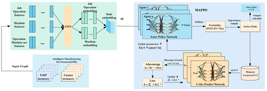
Figure 1.
Architecture of the proposed method.
The specific flow is as follows:
Firstly, when the scheduling event is triggered, the workshop state is inputted into the participant network, and then the q values of the action space are obtained. These q values are then transformed into a probability distribution of action set a using the softmax function, and the production process is then sampled based on this probability distribution. The selected production action is executed in the workshop environment to direct the equipment in completing the task, followed by the receipt of reward and the updated workshop state . Meanwhile, previous scheduling data is stored in the sample pool. The process is repeated until a certain amount of operation data has been stored.
Secondly, the workshop state sensed at the last time step T of the loop in the first step is fed back to the critic network to obtain the state value . Then, the reward set R is obtained via discount factor transformation.
Thirdly, the parameters θ are optimized by calculating the loss function, and then the weight parameters of are updated and optimized based on the backpropagation method.
Finally, the above steps are repeated until all training sets are completed.
In practical situations, there are differences in the probability distributions of the machined workpiece tasks arriving at different equipment on the shop floor. If the network is simply described by shared parameters, it does not reflect the differences between devices, which may lead to problems such as difficulty in converging the results. Therefore, the basic framework used for the MAPPO algorithm module is an improved AC architecture that conforms to the multi-intelligence case by creating different actor networks for different types of intelligence, each maintaining its own network parameters, constituting a multi-actor and a critic architectural model. The process is divided into two main components: centralized training and decentralized execution. During the centralized training phase, each agent learns strategies from its own observations and actions in the environment. The critic neural network gathers current state, action, and environmental information and conveys reward information to multiple participant neural networks. The actor neural network, considering the current state, action, and reward, determines the next action to be executed. All agents communicate with each other, accessing global information and sharing a common evaluation network to assess the value function of agent decisions, aiming for seamless coordination of each agent’s strategy.
After learning, decentralized execution of the model can extract each agent’s local policy from the global policy, making each agent act independently of the others, thus achieving the goal of task assignment and reducing computation time. The output of the policy network in the figure represents the softmax distribution over the entire action space, which corresponds to the probability value of each production action. Subsequently, the production actions are drawn from this probability distribution and executed within the workshop environment. Afterwards, the environment provides the agent with the next workshop state and the corresponding reward to the agent. During model training, data pertaining to states, actions, and rewards extracted from sample trajectories are assembled into a single batch, enabling the policy network to undergo optimization and updating. Upon the arrival of a new task, the intelligence of the same node will make a unified decision regarding the processing task, selecting one machine to carry out the actual matching action, thus mitigating task conflicts among matching decisions.
4.2. Stating Features Embedding
This study uses a graph structure to represent the MDP state, thus capturing the complex relationships between workpiece processes and available equipment. The solution to the job shop scheduling problem is modeled as a heterogeneous graph model (HetG) [48,49], which contains rich information about the arcs between multiple types of nodes and the unstructured content associated with each node. The shop floor graph in Figure 2b can be represented as a heterogeneous graph, where the node types include machine, workpiece, and process as in Figure 2a, and the relationship types include machine–production–workpiece, workpiece–containing–process, and machine–processing–process. Workpieces contain various processes, and the same type of workpieces can be processed on multiple machines of the same type, and machines, workpieces, and processes are interrelated. Therefore a new state feature graph structure ) is defined, where V is a node of multiple operation types, which includes all operations and two virtual operations indicating the start and end of production (with zero processing time), machine nodes are M, each corresponding to a machine , and C is a collection of ensemble arcs, which are directed from the start to the end forming n paths arcs, which represent each processing process of the job. The set of analytic arcs E is an undirected arc that is a link connecting operation nodes and compatible machine nodes. denotes the set of operation object types, and denotes the set of relationship types, and each node is associated with heterogeneous contents, as shown in Figure 2c. Process correlation constraints are also added to enrich the set of connected arcs C and to obtain the tuple form of arc weights by considering inter-process transfer time, machine processing time, and delivery time to represent the state information of the graph nodes.
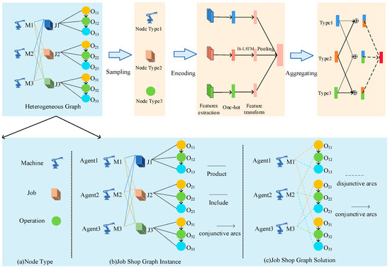
Figure 2.
Heterogeneous graph neural network.
In a real scheduling workshop, the inconsistent size of scheduling instances leads to changes in the size of the state graph, and in order to facilitate the use of deep reinforcement to learn the actual scheduling strategy, the neural structure must be able to operate on state graphs of different sizes. To represent the learning of heterogeneous graphs, this study proposes a new heterogeneous graph neural network model, HetGNN, to obtain the state feature embeddings of nodes in heterogeneous graphs. The original graph neural network approach [50,51], although it can achieve size-agnostic training, is not applicable to solving the heterogeneous graph structure of this study, where any adjacent machine in the heterogeneous graph structure can only be an operation connected by an undirected arc, and operations can be connected to operations and machines by directed or undirected arcs. And the features (i.e., processing time) on the O-M arcs are important. Existing GNNs usually focus only on node features and do not consider arc features. The network model in this study is shown in Figure 2. First, the nodes in HetG are sampled and grouped according to the node types. Then, the feature information of the neighboring nodes sampled in the previous step is aggregated using a heterogeneous graph neural network structure, including machine node embedding and operation node embedding. Finally, a multilayer perceptron is used to train the model. This network structure fully considers the topological and numerical information (original features) of the graph to effectively encode the parsed graph. The graph node embedding method simultaneously considers both node and edge features, preserving different types of relational features in the graph. The node embedding can be viewed as a feature vector, which can perform various final tasks. For graph , node embeddings are calculated by iteratively applying embeddings, and the p-dimensional embeddings of node are calculated by applying embeddings k times. Each embedding layer represents the relationship between different nodes in the graph, and the node v during iteration k is denoted as . The calculation method is as follows:
where is the multilayer perceptron, is the previous node embedding used to distinguish a specific node v from other nodes in the graph, and is the initial node embedding used to consider the initial input features of the target node. ϵ is an arbitrary number, and is the neighborhood of V. A GNN is constructed by stacking k embedding layers, and the p-dimensional vector of the global embedding graph G can be computed from the input graph using the pooling function L after k embedding iterations: . Since solving the dynamic job shop scheduling problem is equivalent to choosing an analytic arc for each node and fixing the direction, that is, the analytic graph associated with each state is a hybrid graph with directed arcs that describe key features such as priority constraints and operation sequences on the machine. The original GNN structure is used for undirected graphs, and the GNN structure needs to be adapted to handle the problem of this study. In the initial state, the undirected analytic arcs are ignored, and then approximate fully directed arcs are added , and as the scheduling process proceeds, increases, implying that more directed arcs are added to the set of approximate directed arcs and the graph is not too dense. At this point, the neighborhood of node V is defined as , where E is the set of arcs of the graph. Finally, the original features of each node on state are defined as , the node embedding obtained after k iterations is denoted as , and the embedding of the graph is denoted as .
Action selection. The proposed graph neural network is used to select an optimal scheduling action at state . In the MDP formulation of the job shop scheduling problem, action represents the assignment of the target task to the available machines, and state represents the information about the shop environment at the transition at step t. To derive the scheduling policy, the actor network is introduced, and MLP is used to obtain the scalar for each action, where has two hidden layers and tanh activation function. The probability distribution of available (feasible) actions selected by the target machine is expected to be generated over the action space, and the actions based on are sampled for training purposes. A softmax function is used during training to calculate the probability of selecting each : . In the process of testing, the sampling strategies are selected using parallelism, and the actions are sampled according to the strategies in each state as well as the greedy E to select the action with the maximum probability. For neural strategies, this parallel approach reduces the additional overhead of sampling.
4.3. Reinforcement Learning Algorithm
As shown in Figure 1, an actor–critic structure is used to train the policy network in the MAPPO algorithm. The actor is the policy network and the critic decision network shares the same graph neural network as the actor. The critic is designed as a case of approximate MLP state values, and the state embedding computed by the graph neural network is used as input to obtain the approximate state value .
Scheduling the initial state as and the interaction time step T between the actor intelligence and the environment, a series of sample trajectories related to the state, action, and reward data are formed and deposited in the sample pool. The cumulative reward is shown in Equation (10), and the probability of each sample trajectory is shown in Equation (11), and the expected reward is . Equation (11) takes the logarithm combined with the expected reward to obtain the strategy gradient of actor, which is calculated as shown in Equation (12):
In Equation (12), is the probability distribution of the corresponding action under the output state of the actor, and is the dominance function at time step t. It is the difference between the action value function and the state value function, reflecting the relative dominance of the selected production action compared with other optional actions. It is calculated as in Equation (13).
In the MAPPO algorithm, the off-policy approach is used to update the strategy, the intelligent body interacts with the environment several times to generate a large amount of data, and the sample trajectories are input to the actor network to obtain the probability distribution of the corresponding action space before and after the state update, respectively, expressed as and , and the similarity between the parameters and is expressed by the weight , which is calculated as in Equation (14), and the final update of the strategy network is updated in the way shown in Equation (15).
When updating, the gradient should try to ensure that the parameters and are equal and limit the update range of the actor network to avoid large differences between the output results due to inconsistent parameters, resulting in abnormal loss function values. Using the clip function for restriction, is the hyperparameter of the (0.1,0.2) interval, and the loss function of the actor is shown in Equation (16).
For the critic network, the critic network loss is the squared loss of the actual state value and the estimated state value in the form of the time difference updated parameter as, as shown in Equation (17), where , so the loss function of critic can also be expressed as the mean squared difference in the values of the dominance function. Via the derivation of the above equation, the corresponding loss function can be derived from the computational Equation (18) to update the agent network.
After initializing the network parameters of the intelligent agent and setting the training hyperparameters, the intelligent agent starts to interact with the environment, stores the data , and completes an episode. Rewards are removed from the storage pool, and the dominance function is constructed. Use the critic network input state of the new agent and obtain the value function , calculate the dominance function according to Equation (13), and finally use Equations (16)–(18) to calculate the total loss function and the gradient algorithm to complete the policy update. The algorithm pseudo-code is as follows, the original sampling is using the same batch of data; here, it is modified to use N actors, where each participant solves a workshop scheduling instance extracted from the distribution D to perform the update. First, I iterations are executed where the DRL agent solves a batch of B instances in parallel (with one replacement every 20 iterations), and then every 10 iterations, the policy is verified on a separate set of validation instances.
The specific Algorithm 1 pseudo-code is as follows.
| Algorithm 1 pseudo-code: MAPPO algorithm |
| Input: set hyperparameters, actor network parameter πθ, critic network parameter vφ, epoch update count R, discount factor γ 1 Sample N instances of workshop scheduling of size B from D 2 for iter = 1, 2…, I do 3 for b = 1, 2…, B do 4 Initialize st based on instance b; 5 while st is not a terminal do 6 extract the embedding using GNN; 7 sampling at in π(at, st); 8 receive the reward rt and the next state st+1; 9 finish updating state st to st+1; 10 compute the advantage function A for each step 11 compute the loss Lppo of PPO and optimize the parameters θ and φ for R epochs 12 update the network parameters; 13 if iter mod 10 = 0 then 14 verify the strategy 15 if iter mod 20 = 0 then 16 sample a new batch of scheduling instances of size B 17 return |
5. Experimental Evaluation
5.1. Experimental Preliminaries
- (1)
- Dataset
Benchmark was used for training and testing, and the datasets selected in this study were as follows:
- (i)
- Brandimarte moderately flexible problem instances [47].
- (ii)
- Three distinct large-scale instance sets, “edata (where few operations can be distributed across more than one machine)”, “rdata (where most operations may be distributed to certain machines)”, and “vdata (where all operations may be distributed to several machines)”, were introduced by Hurink et al. [52].
- (iii)
- Direct testing on larger instances demonstrates the method’s robust generalization. For instance, the DMU instance [53] exhibits a broad range of operation processing times.
- (2)
- Baseline
For each problem of a specific scale, the performance of the proposed method was compared with well-known scheduling rules in the literature. For FJSP, job sorting and disassembly rules and machine assignment scheduling rules are required to complete the planned solution. The job shop scheduling problem, with hundreds of scheduling rules, employs nine heuristic rules derived from pairs of three job scheduling rules and three machine allocation rules as outlined in Reference [54]. These rules include the Shortest Processing Time (SPT), the Shortest Remaining Processing Time (SRPT), the Least Number of Remaining Operations (FOPNR) in the job scheduling rules, and the Earliest Finish Time (EFT), Shortest Processing Time (SPT), and Shortest Processing Time Plus Machine Work (SPTW) in the machine allocation rules. The performance of the proposed method is benchmarked against the top-ranked five combinations, namely FOPNR + SPTW; FOPNR + EFT; SRPT + EFT; SRPT + SPTW; SPT + EFT; and SPT + SPTW. All comparative methods are implemented in Python. For the common benchmark FJSP instance, the gap value Gap uses the latest lower bound UB in the literature [55], and the results of the proposed method are compared with state-of-the-art metaheuristic algorithms, including the improved particle swarm optimization algorithm (HLO-PSO) [56] and the improved genetic algorithm (2S-GA) [57].
- (3)
- Configuration setting
- (i)
- For each problem size, the training strategy network undergoes 20,000 iterations, with each iteration comprising four independent trajectories (i.e., instances), and all original features are normalized to the same scale;
- (ii)
- For the CNN architectures, the network is designed to estimate the Q-value pair . Typical CNN architectures consist of convolutional layers, nonlinear activation layers, and fully connected layers. The convolutional layers used are uniformly partially convolutional filters . The convolutional layers use 16 filters with kernel sizes (1,2), and 100 neurons are used in the fully connected hidden layers. The neural network’s optimizer is Adam. Based on the size of the instances, the hyperparameters beta of 0.9, of and learning rate of . The number of epochs ranges from 50 to 100, depending on the size of the instances. In model design, efforts are made to prevent convergence to local optima during training;
- (iii)
- For the graph neural network GNN with node embedding, for equation , the number of iterations k is set to 2, and is set to 0. Each has 2 hidden layers with a dimension of 64. The action selection network and state value prediction network both have 2 hidden layers with a dimension of 32;
- (iv)
- For DQN, the replay buffer size is set to 20,000, the batch size is set to 64, the discount factor is set to 0.9, and the learning rate is set to 0.001;
- (v)
- For MAPPO, set the epochs of the updated network to 1, set the clipping parameter to 0.2, and set the policy loss L, value function V, and entropy coefficients to 2, 1, and 0.01, respectively. For training, adjust the discount factor to 1 and use an Adam optimizer with a constant learning rate of . Other parameters remain unchanged;
- (vi)
- The hardware is a machine equipped with an Intel(R) Xeon(R) Gold 6130 CPU and a single Nvidia GeForce 3080Ti GPU.
5.2. Experimental Result
In this section, comparative experiments are conducted to show the decision differences between the scheduling architecture proposed in this study and the single intelligent scheduling architecture in terms of the overall scheduling optimization objective makespan, the stability of the trained architecture, and the machine resource allocation capability. The experimental results show that the method outperforms the manual design rule and the RL-based single-intelligent scheduling architecture in terms of the overall algorithm performance, the stability of the trained architecture, and the machine resource allocation capability.
- (1)
- Performance evaluation of algorithms
The comparison of the method proposed in this study with the manually designed scheduling rules and other reinforcement learning algorithms, respectively, is statistically presented, and the results of the algorithm on instances of different sizes are shown in Table 1 and Table 2 and Figure 3a,b. A scheduling capability of the method proposed in this study and other reinforcement learning algorithms on unseen instances is compared as shown in Table 3 for 10 DMU instances, which are divided into 2 groups according to their sizes for the experiments. To highlight the effect, the generalization performance of 20 × 15 and 20 × 20 instances in Table 3 is presented.

Table 1.
Comparison results with scheduling rules on medium and large-scale instances (The numbers in the table represent the processing time of the dataset under each experimental method, while bold numbers represent the results of our experimental method. The closer the distribution of bold numbers, the stronger the effectiveness of our proposed method on large-scale datasets compared to other methods in the table).
Table 2.
Comparison results with reinforcement learning algorithms on medium and large-scale instances (The numbers in the table represent the processing time of the dataset under each experimental method, and the bold numbers represent the effectiveness of our experimental method results on medium to large-scale datasets).
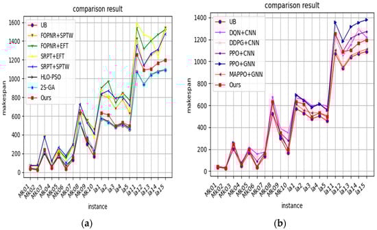
Figure 3.
(a) Comparison with scheduling rules. (b) Comparison with reinforcement learning algorithms.
Table 3.
Comparison of scheduling results on DMU instances (The numbers in the table represent the processing time of the dataset under each experimental method, and the bold numbers represent the generalization of the results of our experimental method on invisible datasets).
The following conclusions are made:
- (i)
- In all instances, DRL significantly outperforms the best rule, and the algorithm has stronger generalization;
- (ii)
- The performance of the scheduling rule is unstable on Hurink’s instances and Brandimarte’s instances. From the experimental results, it can be seen that on Hurink’s instance, the scheduling rules with better performance are FOPNR + SPTW and SRPT + SPTW, and from the mean value, FOPNR + EFT and SRPT + EFT on Brandimarte’s instance perform better; in contrast, the method proposed in this study shows some stability for public instances.
- (iii)
- It can be found that the DRL method significantly outperforms all scheduling rules when trained on small-scale instances and generalized on large-scale instances, indicating that the method proposed in this study is effective when dealing with high-dimensional input space; and for the whole learning process, DMU is the data used for testing, and it can be seen from the experimental data that the method proposed in this study can effectively learn to generate better for invisible instances solutions.
- (iv)
- Tested with the same parameters, the PPO algorithm [44] performs better on instances than DQN [41] and DDPG [58] and performs about the same as the metaheuristic on instances with a relatively small total number of JXMs but for larger instances, the performance of the method proposed in this study is significantly better. However, overall, regardless of the method used, the ability to solve large-scale problems is worse than the ability to solve small-scale problems, and the training error increases as the scale increases in comparison to DRL. The increase in problem size brings about an increase in the scheduling state space, and the learning error increases when using the same network structure, such as CNN, which requires more iterations and a more optimized network structure to reduce the training error. So, it also reflects that using an improved graph neural network structure can reduce the training error, adapt to different sizes of data input, and improve the training speed.
- (2)
- Energy consumption assessment
Consider evaluating the overall algorithm when dynamic events occur, and to facilitate the comparison effect, use the dataset 5J5M [59] for testing. The data include the operation priority and available energy consumption of five jobs, as well as the assigned machine numbers and the idle power of five machines.
In order to evaluate the different impacts of dynamic events on the overall algorithm performance, two scenarios were considered, including insertion of orders and machine failures. In the above sequence, workpiece 5 was added as an insertion order, using a sequential insertion method, considering that the production process can be interrupted. At time point T = 20, it was used as an insertion point with a delivery time of 30, and the inserted order processing was added to the overall scheduling process as a scheduling interval. When considering machine failure, it is assumed that machine 1 breaks down in 10 s, and the repair time is 20. The operations involved in the tasks that need to be handled on the faulty machine can be directly transferred to other machines with equivalent processing capabilities. This article proposes that after repair, there is no need to wait for the faulty machine to continue processing the operations involved, greatly reducing the completion time. As shown in Figure 4, it is a Gantt chart after inserting orders and machine failures. To evaluate the performance of our proposed optimization method, we compared the energy consumption of the proposed algorithm with optimization using NSGA-II [28] and PSO [60] algorithms. From Figure 5 and Figure 6, it can be seen that our algorithm has an energy consumption advantage in the case of single insertion and machine failure, respectively.
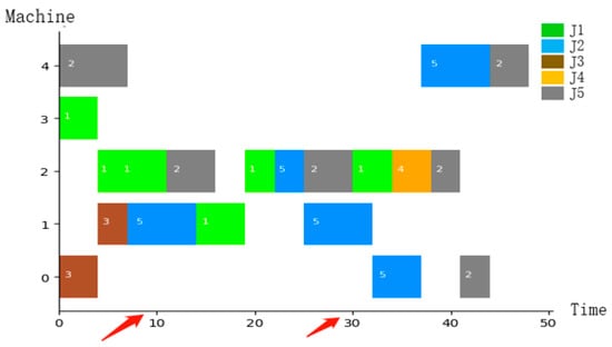
Figure 4.
Gantt chart for inserting orders and machine failures.
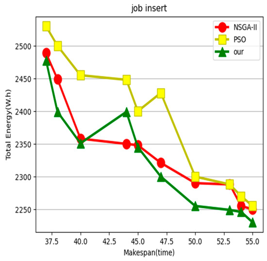
Figure 5.
Insertion situation.
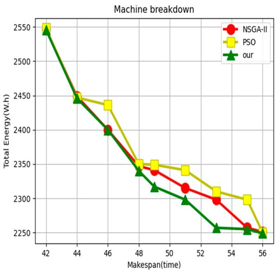
Figure 6.
Machine fault situation.
- (3)
- Performance evaluation of the architecture
A single-intelligence architecture will contain all combined actions of all artifact orders, resulting in a huge action space requiring deep neural networks with high complexity. The multi-intelligence architecture can solve the drawback of large space by transferring the complexity of action space to the difficulty of collaboration among intelligence, so this study builds a new distributed multi-agent scheduling architecture (DMASA) in order to verify the advantage of the new architecture over single-agent In order to verify the advantages of the new architecture over the single-agent scheduling architecture, it is compared with the distributed single-agent architecture (DSASA) in terms of training stability. For the RL-based scheduling algorithm, the training stability reflects the repeatability and reliability of the RL model. The PPO algorithms under both architectures are trained independently, the average of 8 independent results is taken, the episode is evaluated every 100 training steps, and the average completion rate of the independent runs is taken for comparison, with the vertical coordinate being the average completion rate. For the convenience of viewing the comparison effect, the training experiment results of MK01 (10J6M) and MK03 (15J8M) datasets are picked out as shown in Figure 7. The DSASA variation is large, and the training is not as stable as MASA, although they both converge to stable values after several episodes; it can be found that the MASA curve is turbulent, and the MASA curve shows a stable upward trend. Thus, MASA is more stable and reliable than DSASA, confirming that the multi-intelligence architecture used in this study is advantageous.
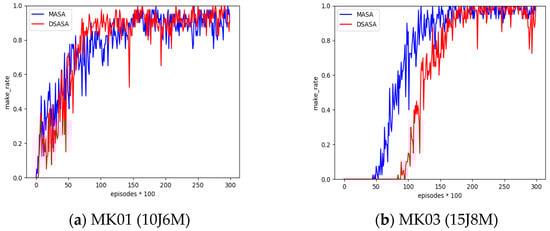
Figure 7.
Training stability.
- (4)
- Evaluation of machine resource allocation
A scheduling result Gantt chart is drawn to represent the processing during the scheduling process to show the detailed results as shown in Figure 8 and Figure 9. To facilitate viewing the comparison results, the same data sets MK01 (10J6M) and MK03 (15J8M) as in part (2) are used. The bars indicate the processing of the processes in the job, the length indicates the processing time, and the vertical coordinate is the list of devices. The Gantt chart in Figure 8 shows the order in which 10 tasks are assigned to 6 machines, with different tasks represented by icons of different colors. The chart on the right shows the situation of single agent scheduling, with two rows of scheduling sequences, upper and lower. The completion time of the last process after processing can be seen as 42 on the left and 46 on the right from the Gantt chart. Similarly, the completion time after the completion of the last process in Figure 9 can be seen from the Gantt chart as 243 on the left and 255 on the right. From the experimental results, it can be seen that under our method’s scheduling architecture, machine allocation is relatively tight. In (a), the degree of machine equipment differentiation is greater than in (b), and it has an advantage in completion time. From the experimental results, we can see that under the scheduling architecture of our method, the machines are assigned more closely, and in (a), the machines and devices are equally divided than in (b). Our scheduling architecture considers the global state and the single-intelligence scheduling architecture only considers the individual rewards of each agent, which leads to poorer scheduling results.
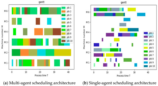
Figure 8.
Gantt chart of scheduling results under two scheduling architectures (MK01 10J6M).
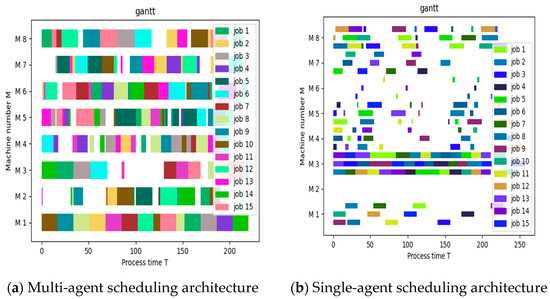
Figure 9.
Gantt chart of scheduling results under two scheduling architectures (MK03 15J8M).
- (5)
- Verification of actual processing workshop
Build a physical platform for processing specific products on actual production lines, achieving connectivity, interaction, and real-time monitoring and retrieval of various equipment. Three types of products, each containing multiple models, can be produced on mixed production lines without stopping the machine. The products to be produced include customizable Bluetooth selfies, customizable USB drives, and customizable wooden carving handicraft pendants. Customers can choose the body and lid of the packaging box used to package these products. Products that customers choose to process or assemble can be placed in their own packaging boxes. The final product consists of three types of products and packaging boxes of different colors, forming several types of gift boxes. The two perspectives of the actual machining platform are shown in Figure 10.
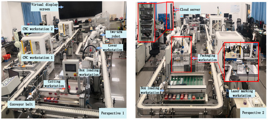
Figure 10.
Product processing platform. The actual production line can achieve mixed production of three types of products, each containing multiple models of products. The proposed products include customizable Bluetooth selfies, customizable USB drives, and customizable wooden carving handicraft pendants.
In the actual processing environment validation, using data from an actual production line as shown in Appendix A, the same algorithm was used for model training. The loss function changes during the training phase were visualized, as shown in Figure 11. the change in the loss function reflects whether the algorithm model converges during the training phase. Due to the instability that often occurs during the training phase of the graph neural network used, attention needs to be paid to the change in the loss function., and the final scheduling result Gantt chart was created; the Gantt chart displays 1 and 2 indicating that different processes of the product are assigned to different processing machines for processing. The final actual production line scheduling results are shown in Figure 12, achieving the implementation of processing.
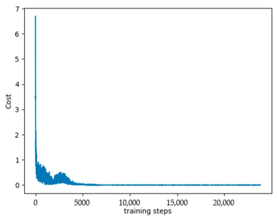
Figure 11.
Visualization of loss function changes during the training phase.
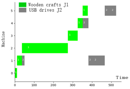
Figure 12.
Actual production line scheduling results.
6. Conclusions
In response to the current challenges and problems in the field of intelligent production scheduling, this study focuses on solving the dynamic job shop scheduling problem in intelligent manufacturing, scheduling and rescheduling received orders as quickly as possible under the perturbation of orders and resources while satisfying the requirements of multi-objective optimization, modeling the required problem as a multi-intelligent dynamic shop scheduling problem, in order to achieve a reasonable allocation of production tasks and manufacturing resources to maximize The scheduling optimization objectives such as minimizing completion time, reducing production energy consumption, and achieving load balancing are accomplished to the maximum extent. In this study, each workpiece is considered as an intelligent body, and a reinforcement learning algorithm is used to realize the collaboration among all intelligent bodies, maximize the global reward, effectively train and implement the scheduling algorithm, and complete the scheduling decision. (DMASA), an end-to-end multi-agent deep reinforcement learning method (MADRL) is proposed to solve the multi-intelligent dynamic shop floor scheduling problem, and the representation of states, actions, observations and rewards is introduced based on the Markov decision formula, and an improved parsing graph is proposed to represent the states, and a heterogeneous graph neural network (HGNN) is used to encode state nodes, thus efficiently computing strategies, including machine matching strategies and process selection strategies. Based on the improved graph neural network, the AC architecture is used, and it is trained with MAPPO. Extensive experiments on common instances and standard benchmarks show that the experimental results demonstrate that the proposed method outperforms traditional scheduling methods, is reasonably efficient, and generalizes well to larger-scale unseen instances and instances from public benchmarks.
This article validates the effectiveness of the proposed method on one’s actual production line, and future work will focus on two aspects. (1) Although the DMASA architecture has obvious effects and some techniques have been used in training, the training efficiency still needs to be improved. HGNN requires high computational costs, and MARL training requires both CPU and GPU. Therefore, future work will be based on distributed computing devices for experimentation and evaluation of scheduling performance when scheduling dozens or hundreds of tasks. (2) Considering the changing environment of the actual processing workshop, there will be more practical constraints, including waiting time regulations, batch processing of workshop operations, etc. However, the formulas in the current article have not taken into account more practical constraints. The constraint conditions can be extended to the MDP formula for a state transition to comply with additional constraints. The reward function can also be modified to cope with the extension of the MDP formula. By adding terminal rewards that consider average delay or flow time to the proposed reward settings, future research will expand the MDP formula by adding constraints that are more in line with the actual workshop environment, providing a new perspective for task decomposition and subtask learning in actual MARL.
Author Contributions
Y.P.: Conceptualization, Methodology, Software, Validation, Writing—First Draft, Formal Analysis, Survey. F.L.: Conceptualization, Methodology, Validation, Writing—Review and Editing, Supervision. S.R.: Resources, Writing standards, English verification—review and editing, supervision. All authors have read and agreed to the published version of the manuscript.
Funding
This work is partially supported by the Natural Science Foundation of Guangdong Province (2023A1515011173, 2021A1515012126), Guangzhou Science and Technology Plan Project (202206030008), National Key R&D Project (No. 2018YFB1700500); Open Project Fund of the Key Laboratory of Big Data and Intelligent Robot of the Ministry of Education (202101).
Institutional Review Board Statement
Not applicable.
Informed Consent Statement
Not applicable.
Data Availability Statement
The data presented in this study are available on request from the corresponding author.
Conflicts of Interest
The authors declare no conflicts of interest.
Abbreviations
| DMASA | Distributed Multi-Agent Scheduling Architecture |
| HGNN | Heterogeneous Graph Neural Network |
| AC | Actor–Critic |
| RL | Reinforcement Learning |
| DRL | Deep Reinforcement Learning |
| GE-HetGNN | Graph Embedding–Heterogeneous Graph Neural Network |
| HetG | Heterogeneous Graphs |
| MAPPO | Multi-Agent Proximal Policy Optimization |
| MADRL | Multi-Agent Deep Reinforcement Learning |
| GA | Genetic Algorithms |
| PSO | Particle Swarm Optimization |
| ACO | Ant Colony Optimization |
| ANN | Artificial Neural Network |
Appendix A
Table A1.
Actual production line data.
Table A1.
Actual production line data.
| Job Agent | Operation Sequence | Processing Machines and Time Consumption | |||||
|---|---|---|---|---|---|---|---|
| Wooden Crafts | Upper box | 11.44 | 13 | 14 | - | - | - |
| Feeding | - | 25.14 | 26 | 27 | 30 | - | |
| CNC1, CNC2 | 240 | 242 | 238.46 | - | - | - | |
| Packing | 60 | 61 | - | 50.38 | - | - | |
| Upper cover | 28 | - | 30 | - | 26.19 | 32 | |
Cutting materials | - | 28 | 36 | - | - | 26.84 | |
| USB drives | Upper box | 11.44 | 13 | 14 | - | - | |
| Feeding | - | 25.14 | 26 | 27 | 30 | - | |
| Laser | 19 | 24 | 18.21 | - | - | - | |
| Packing | 60 | 61 | - | 50.38 | - | ||
| Upper cover | 28 | - | 30 | - | 26.19 | 32 | |
Cutting materials | - | 28 | 36 | - | - | 26.84 | |
References
- Zhang, J.; Ding, G.; Zou, Y.; Qin, S.; Fu, J. Review of job shop scheduling research and its new perspectives under Industry 4.0. J. Intell. Manuf. 2019, 30, 1809–1830. [Google Scholar] [CrossRef]
- Azemi, F.; Tokody, D.; Maloku, B. An optimization approach and a model for Job Shop Scheduling Problem with Linear Programming. In Proceedings of the UBT International Conference 2019, Pristina, Kosovo, 26 October 2019. [Google Scholar]
- Sels, V.; Gheysen, N.; Vanhoucke, M. A comparison of priority rules for the job shop scheduling problem under different flow time-and tardiness-related objective functions. Int. J. Prod. Res. 2012, 50, 4255–4270. [Google Scholar] [CrossRef]
- Park, J.; Chun, J.; Kim, S.H.; Kim, Y.; Park, J. Learning to schedule job-shop problems: Representation and policy learning using graph neural network and reinforcement learning. Int. J. Prod. Res. 2021, 59, 3360–3377. [Google Scholar] [CrossRef]
- Nasiri, M.M.; Salesi, S.; Rahbari, A.; Salmanzadeh Meydani, N.; Abdollai, M. A data mining approach for population-based methods to solve the JSSP. Soft Comput. 2019, 23, 11107–11122. [Google Scholar] [CrossRef]
- Mao, H.; Schwarzkopf, M.; Venkatakrishnan, S.B.; Meng, Z.; Alizadeh, M. Learning scheduling algorithms for data processing clusters. In Proceedings of the ACM Special Interest Group on Data Communication, Beijing, China, 19–23 August 2019; pp. 270–288. [Google Scholar]
- Wang, J.; Zhang, Y.; Liu, Y.; Wu, N. Multiagent and bargaining-game-based real-time scheduling for internet of things-enabled flexible job shop. IEEE Internet Things J. 2018, 6, 2518–2531. [Google Scholar] [CrossRef]
- Wang, Z.; Gombolay, M. Learning scheduling policies for multi-robot coordination with graph attention networks. IEEE Robot. Autom. Lett. 2020, 5, 4509–4516. [Google Scholar] [CrossRef]
- Hu, H.; Jia, X.; He, Q.; Fu, S.; Liu, K. Deep reinforcement learning based AGVs real-time scheduling with mixed rule for flexible shop floor in industry 4.0. Comput. Ind. Eng. 2020, 149, 106749. [Google Scholar] [CrossRef]
- Caldeira, R.H.; Gnanavelbabu, A.; Vaidyanathan, T. An effective backtracking search algorithm for multi-objective flexible job shop scheduling considering new job arrivals and energy consumption. Comput. Ind. Eng. 2020, 149, 106863. [Google Scholar] [CrossRef]
- Kong, M.; Xu, J.; Zhang, T.; Lu, S.; Fang, C.; Mladenovic, N. Energy-efficient rescheduling with time-of-use energy cost: Application of variable neighborhood search algorithm. Comput. Ind. Eng. 2021, 156, 107286. [Google Scholar] [CrossRef]
- Yin, S.; Xiang, Z. Adaptive operator selection with dueling deep Q-network for evolutionary multi-objective optimization. Neurocomputing 2024, 581, 127491. [Google Scholar] [CrossRef]
- Mangalampalli, S.; Karri, G.R.; Kumar, M.; Khalaf, O.I.; Romero, C.A.; Sahib, G.A. DRLBTSA: Deep reinforcement learning based task-scheduling algorithm in cloud computing. Multimed. Tools Appl. 2024, 83, 8359–8387. [Google Scholar] [CrossRef]
- Gui, Y.; Tang, D.; Zhu, H.; Zhang, Y.; Zhang, Z. Dynamic scheduling for flexible job shop using a deep reinforcement learning approach. Comput. Ind. Eng. 2023, 180, 109255. [Google Scholar] [CrossRef]
- Srinath, N.; Yilmazlar, I.O.; Kurz, M.E.; Taaffe, K. Hybrid multi-objective evolutionary meta-heuristics for a parallel machine scheduling problem with setup times and preferences. Comput. Ind. Eng. 2023, 185, 109675. [Google Scholar] [CrossRef]
- Kianfar, K.; Atighehchian, A. A hybrid heuristic approach to master surgery scheduling with downstream resource constraints and dividable operating room blocks. Ann. Oper. Res. 2023, 328, 727–754. [Google Scholar] [CrossRef]
- Chen, M.; Tan, Y. SF-FWA: A Self-Adaptive Fast Fireworks Algorithm for effective large-scale optimization. Swarm Evol. Comput. 2023, 80, 101314. [Google Scholar] [CrossRef]
- Wang, G.; Wang, P.; Zhang, H. A Self-Adaptive Memetic Algorithm for Distributed Job Shop Scheduling Problem. Mathematics 2024, 12, 683. [Google Scholar] [CrossRef]
- Cimino, A.; Elbasheer, M.; Longo, F.; Mirabelli, G.; Padovano, A.; Solina, V. A Comparative Study of Genetic Algorithms for Integrated Predictive Maintenance and Job Shop Scheduling. In Proceedings of the European Modeling and Simulation Symposium, EMSS, Santo Stefano, Italy, 18–20 September 2023. [Google Scholar]
- Dulebenets, M.A. An Adaptive Polyploid Memetic Algorithm for scheduling trucks at a cross-docking terminal. Inf. Sci. 2021, 565, 390–421. [Google Scholar] [CrossRef]
- Singh, P.; Pasha, J.; Moses, R.; Sobanjo, J.; Ozguven, E.E.; Dulebenets, M.A. Development of exact and heuristic optimization methods for safety improvement projects at level crossings under conflicting objectives. Reliab. Eng. Syst. Saf. 2022, 220, 108296. [Google Scholar] [CrossRef]
- Singh, E.; Pillay, N. A study of ant-based pheromone spaces for generation constructive hyper-heuristics. Swarm Evol. Comput. 2022, 72, 101095. [Google Scholar] [CrossRef]
- Jing, X.; Pan, Q.; Gao, L. Local search-based metaheuristics for the robust distributed permutation flowshop problem. Appl. Soft Comput. 2021, 105, 107247. [Google Scholar] [CrossRef]
- Luo, J.; El Baz, D.; Xue, R.; Hu, J. Solving the dynamic energy aware job shop scheduling problem with the heterogeneous parallel genetic algorithm. Future Gener. Comput. Syst. 2020, 108, 119–134. [Google Scholar] [CrossRef]
- Xu, B.; Mei, Y.; Wang, Y.; Ji, Z.; Zhang, M. Genetic programming with delayed routing for multiobjective dynamic flexible job shop scheduling. Evol. Comput. 2021, 29, 75–105. [Google Scholar] [CrossRef]
- Nguyen, S.; Mei, Y.; Xue, B.; Zhang, M. A hybrid genetic programming algorithm for automated design of dispatching rules. Evol. Comput. 2019, 27, 467–496. [Google Scholar] [CrossRef] [PubMed]
- Zhang, F.; Mei, Y.; Nguyen, S.; Zhang, M. Correlation coefficient-based recombinative guidance for genetic programming hyperheuristics in dynamic flexible job shop scheduling. IEEE Trans. Evol. Comput. 2021, 25, 552–566. [Google Scholar] [CrossRef]
- Li, Y.; He, Y.; Wang, Y.; Tao, F.; Sutherland, J.W. An optimization method for energy-conscious production in flexible machining job shops with dynamic job arrivals and machine breakdowns. J. Clean. Prod. 2020, 254, 120009. [Google Scholar] [CrossRef]
- Li, Z.; Chen, Y. Minimizing the makespan and carbon emissions in the green flexible job shop scheduling problem with learning effects. Sci. Rep. 2023, 13, 6369. [Google Scholar] [CrossRef] [PubMed]
- Shao, W.; Shao, Z.; Pi, D. A multi-neighborhood-based multi-objective memetic algorithm for the energy-efficient distributed flexible flow shop scheduling problem. Neural Comput. Appl. 2022, 34, 22303–22330. [Google Scholar] [CrossRef]
- Afsar, S.; Palacios, J.J.; Puente, J.; Vela, C.R.; Gonzalez-Rodriguez, I. Multi-objective enhanced memetic algorithm for green job shop scheduling with uncertain times. Swarm Evol. Comput. 2022, 68, 101016. [Google Scholar] [CrossRef]
- Mnih, V.; Kavukcuoglu, K.; Silver, D.; Rusu, A.A.; Veness, J.; Bellemare, M.G.; Graves, A.; Riedmiller, M.; Fidjeland, A.K.; Ostrovski, G.; et al. Human-level control through deep reinforcement learning. Nature 2015, 518, 529–533. [Google Scholar] [CrossRef]
- Akyol, D.E.; Bayhan, G.M. A review on evolution of production scheduling with neural networks. Comput. Ind. Eng. 2007, 53, 95–122. [Google Scholar] [CrossRef]
- Weckman, G.R.; Ganduri, C.V.; Koonce, D.A. A neural network job-shop scheduler. J. Intell. Manuf. 2008, 19, 191–201. [Google Scholar] [CrossRef]
- Gong, G.; Chiong, R.; Deng, Q.; Gong, X.; Lin, W.; Han, W.; Zhang, L. A two-stage memetic algorithm for energy-efficient flexible job shop scheduling by means of decreasing the total number of machine restarts. Swarm Evol. Comput. 2022, 75, 101131. [Google Scholar] [CrossRef]
- Park, I.B.; Huh, J.; Kim, J.; Park, J. A reinforcement learning approach to robust scheduling of semiconductor manufacturing facilities. IEEE Trans. Autom. Sci. Eng. 2019, 17, 1420–1431. [Google Scholar] [CrossRef]
- Xiong, H.; Fan, H.; Jiang, G.; Li, G. A simulation-based study of dispatching rules in a dynamic job shop scheduling problem with batch release and extended technical precedence constraints. Eur. J. Oper. Res. 2017, 257, 13–24. [Google Scholar] [CrossRef]
- Ning, T.; Huang, M.; Liang, X.; Jin, H. A novel dynamic scheduling strategy for solving flexible job-shop problems. J. Ambient Intell. Humaniz. Comput. 2016, 7, 721–729. [Google Scholar] [CrossRef]
- Baykasoglu, A.; Karaslan, F.S. Solving comprehensive dynamic job shop scheduling problem by using a GRASP-based approach. Int. J. Prod. Res. 2017, 55, 3308–3325. [Google Scholar] [CrossRef]
- Liu, Y.; Fan, J.; Zhao, L.; Shen, W.; Zhang, C. Integration of deep reinforcement learning and multi-agent system for dynamic scheduling of re-entrant hybrid flow shop considering worker fatigue and skill levels. Robot. Comput.-Integr. Manuf. 2023, 84, 102605. [Google Scholar] [CrossRef]
- Workneh, A.D.; Gmira, M. Learning to schedule (L2S): Adaptive job shop scheduling using double deep Q network. Smart Sci. 2023, 11, 409–423. [Google Scholar] [CrossRef]
- Luo, S. Dynamic scheduling for flexible job shop with new job insertions by deep reinforcement learning. Appl. Soft Comput. 2020, 91, 106208. [Google Scholar] [CrossRef]
- Liu, C.; Chang, C.; Tseng, C. Actor-critic deep reinforcement learning for solving job shop scheduling problems. IEEE Access 2020, 8, 71752–71762. [Google Scholar] [CrossRef]
- Zhang, Y.; Zhu, H.; Tang, D.; Zhou, T.; Gui, Y. Dynamic job shop scheduling based on deep reinforcement learning for multi-agent manufacturing systems. Robot. Comput. Integr. Manuf. 2022, 78, 102412. [Google Scholar] [CrossRef]
- Han, B.; Yang, J. Research on adaptive job shop scheduling problems based on dueling double DQN. IEEE Access 2020, 8, 186474–186495. [Google Scholar] [CrossRef]
- Huang, J.; Gao, L.; Li, X. An end-to-end deep reinforcement learning method based on graph neural network for distributed job-shop scheduling problem. Expert Syst. Appl. 2024, 238, 121756. [Google Scholar] [CrossRef]
- Brandimarte, P. Routing and scheduling in a flexible job shop by tabu search. Ann. Oper. Res. 1993, 41, 157–183. [Google Scholar] [CrossRef]
- Sun, Y.; Han, J.; Yan, X.; Yu, P.S.; Wu, T. Pathsim: Meta path-based top-k similarity search in heterogeneous information networks. Proc. VLDB Endow. 2011, 4, 992–1003. [Google Scholar] [CrossRef]
- Sun, Y.; Norick, B.; Han, J.; Yan, X.; Yu, P.S.; Yu, X. Pathselclus: Integrating meta-path selection with user-guided object clustering in heterogeneous information networks. ACM Trans. Knowl. Discov. Data (TKDD) 2013, 7, 1–23. [Google Scholar] [CrossRef]
- Zhang, C.; Song, W.; Cao, Z.; Zhang, J.; Tan, P.S.; Chi, X. Learning to dispatch for job shop scheduling via deep reinforcement learning. Adv. Neural Inf. Process. Syst. 2020, 33, 1621–1632. [Google Scholar]
- Ni, F.; Hao, J.; Lu, J.; Tong, X.; Yuan, M.; Duan, J.; Ma, Y.; He, K. A multi-graph attributed reinforcement learning based optimization algorithm for large-scale hybrid flow shop scheduling problem. In Proceedings of the 27th ACM SIGKDD Conference on Knowledge Discovery & Data Mining, Singapore, 14–18 August 2021. [Google Scholar]
- Hurink, J.; Jurisch, B.; Thole, M. Tabu search for the job-shop scheduling problem with multi-purpose machines. Oper.-Res.-Spektrum 1994, 15, 205–215. [Google Scholar] [CrossRef]
- Jain, A.S.; Meeran, S. Deterministic job-shop scheduling: Past, present and future. Eur. J. Oper. Res. 1999, 113, 390–434. [Google Scholar] [CrossRef]
- Han, B.; Yang, J. A deep reinforcement learning based solution for flexible job shop scheduling problem. Int. J. Simul. Model. 2021, 20, 375–386. [Google Scholar] [CrossRef]
- Behnke, D.; Geiger, M.J. Test Instances for the Flexible Job Shop Scheduling Problem with Work Centers. Arbeitspapier/Research Paper/Helmut-Schmidt-Universitat, Lehrstuhl fur Betriebswirtschaftslehre, Insbes. Logistik-Management. 2012. Available online: https://d-nb.info/1023241773/34 (accessed on 1 February 2024).
- Ding, H.; Gu, X. Hybrid of human learning optimization algorithm and particle swarm optimization algorithm with scheduling strategies for the flexible job-shop scheduling problem. Neurocomputing 2020, 414, 313–332. [Google Scholar] [CrossRef]
- Rooyani, D.; Defersha, F.M. An efficient two-stage genetic algorithm for flexible job-shop scheduling. IFAC Pap. 2019, 52, 2519–2524. [Google Scholar] [CrossRef]
- Lu, R.; Li, Y.-C.; Li, Y.; Jiang, J.; Ding, Y. Multi-agent deep reinforcement learning based demand response for discrete manufacturing systems energy management. Appl Energy 2020, 276, 115473. [Google Scholar] [CrossRef]
- He, Y.; Li, Y.; Wu, T.; Sutherland, J.W. An energy-responsive optimization method for machine tool selection and operation sequence in flexible machining job shops. J. Clean. Prod. 2015, 87, 245–254. [Google Scholar] [CrossRef]
- Nouiri, M.; Bekrar, A.; Trentesaux, D. Towards Energy Efficient Scheduling and Rescheduling for Dynamic Flexible Job Shop Problem. IFAC-Pap. 2018, 51, 1275–1280. [Google Scholar] [CrossRef]
Disclaimer/Publisher’s Note: The statements, opinions and data contained in all publications are solely those of the individual author(s) and contributor(s) and not of MDPI and/or the editor(s). MDPI and/or the editor(s) disclaim responsibility for any injury to people or property resulting from any ideas, methods, instructions or products referred to in the content. |
© 2024 by the authors. Licensee MDPI, Basel, Switzerland. This article is an open access article distributed under the terms and conditions of the Creative Commons Attribution (CC BY) license (https://creativecommons.org/licenses/by/4.0/).