Author Contributions
Conceptualization and design of the study, M.L.; data extraction and data curation, M.L., A.S., U.P., S.P. and R.M.; formal analysis M.L., A.S., S.P., R.M. and A.R.C.; visualization, M.L., D.N., A.S., S.P., R.M., S.D.L. and S.M.; validation, M.L., D.N., A.S., S.P., R.M. and A.R.C.; writing—original draft, M.L.; writing—review and editing, S.M. and D.N.; supervision, M.L., A.R.C., D.N. and S.M.; project administration, M.L. and D.N.; funding acquisition, D.N. All authors have read and agreed to the published version of the manuscript.
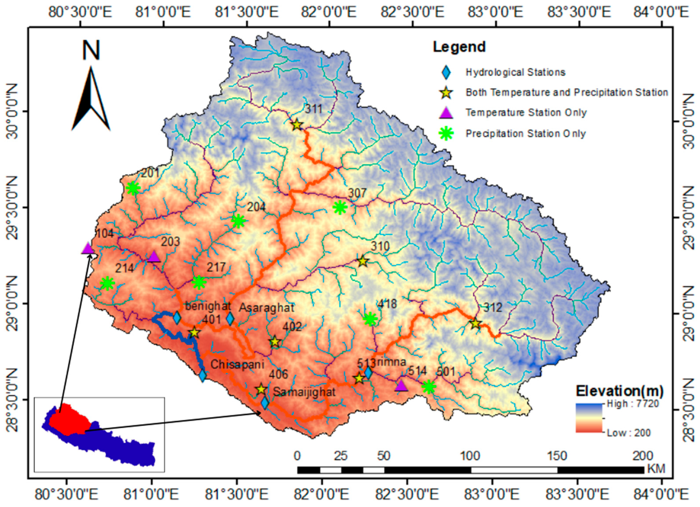
Figure 1.
Map of the KRB showcasing the extensive river network and the locations of rainfall, temperature, and discharge monitoring stations, superimposed on a 30 m resolution Digital Elevation Model (DEM) to highlight the topographical context.
Figure 1.
Map of the KRB showcasing the extensive river network and the locations of rainfall, temperature, and discharge monitoring stations, superimposed on a 30 m resolution Digital Elevation Model (DEM) to highlight the topographical context.
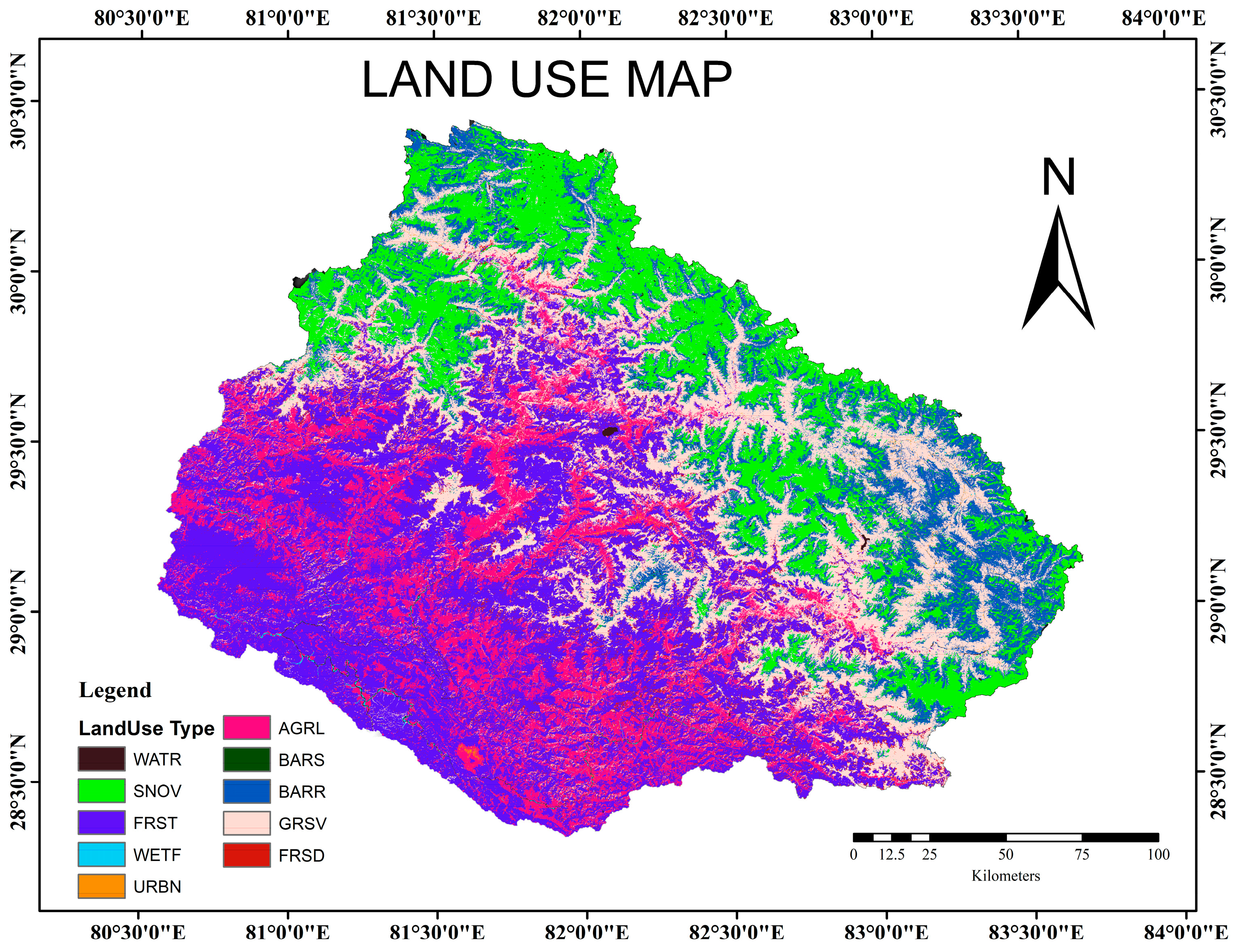
Figure 2.
Land cover map across the KRB shows that FRST (Forest), GRSV (Grassland), SNOV (Snow and Ice), AGRL (Agriculture), and BARR (Barren Land) are the major land use types present in the study area.
Figure 2.
Land cover map across the KRB shows that FRST (Forest), GRSV (Grassland), SNOV (Snow and Ice), AGRL (Agriculture), and BARR (Barren Land) are the major land use types present in the study area.
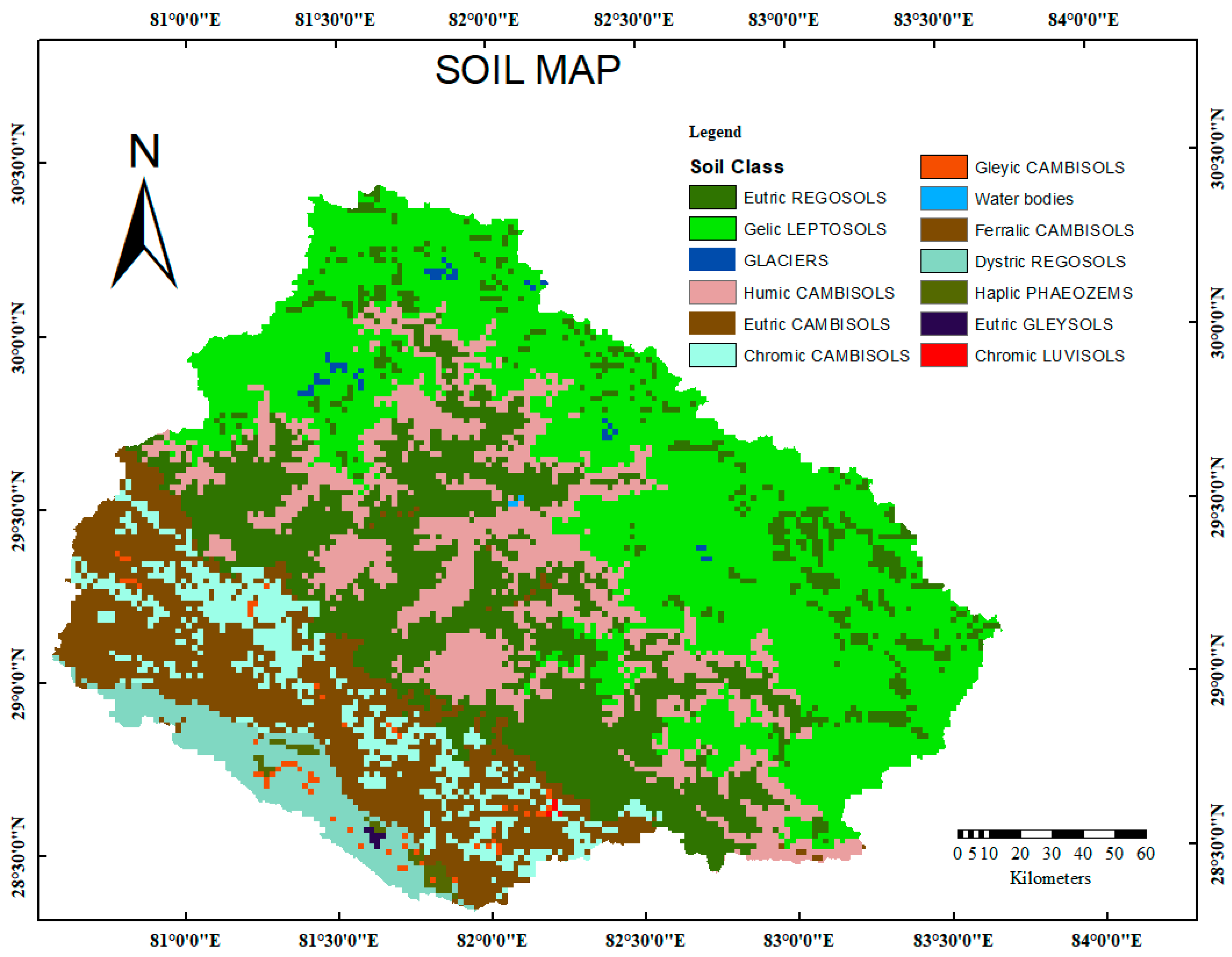
Figure 3.
Map showing the soil types present across the KRB, with Gelic LEPTOSOL, Eutric REGOSOLS, Humic CAMBISOLS, Eutric CAMBISOLS, and Chromic CAMBISOLS as the primary soil types present in the study area.
Figure 3.
Map showing the soil types present across the KRB, with Gelic LEPTOSOL, Eutric REGOSOLS, Humic CAMBISOLS, Eutric CAMBISOLS, and Chromic CAMBISOLS as the primary soil types present in the study area.
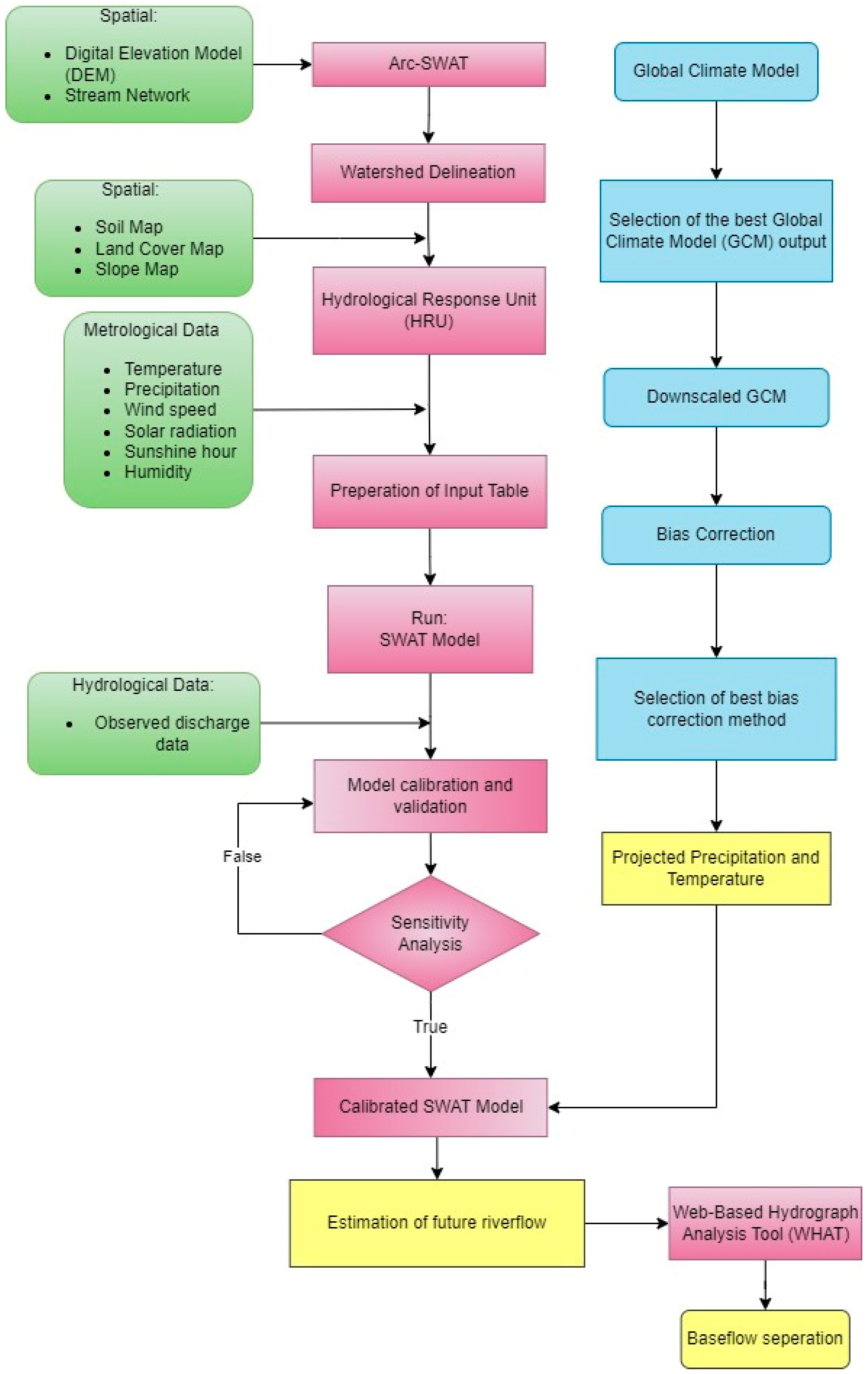
Figure 4.
Flowchart illustrating the systematic methodology applied in this study, detailing the step-by-step investigative processes and analytical techniques.
Figure 4.
Flowchart illustrating the systematic methodology applied in this study, detailing the step-by-step investigative processes and analytical techniques.
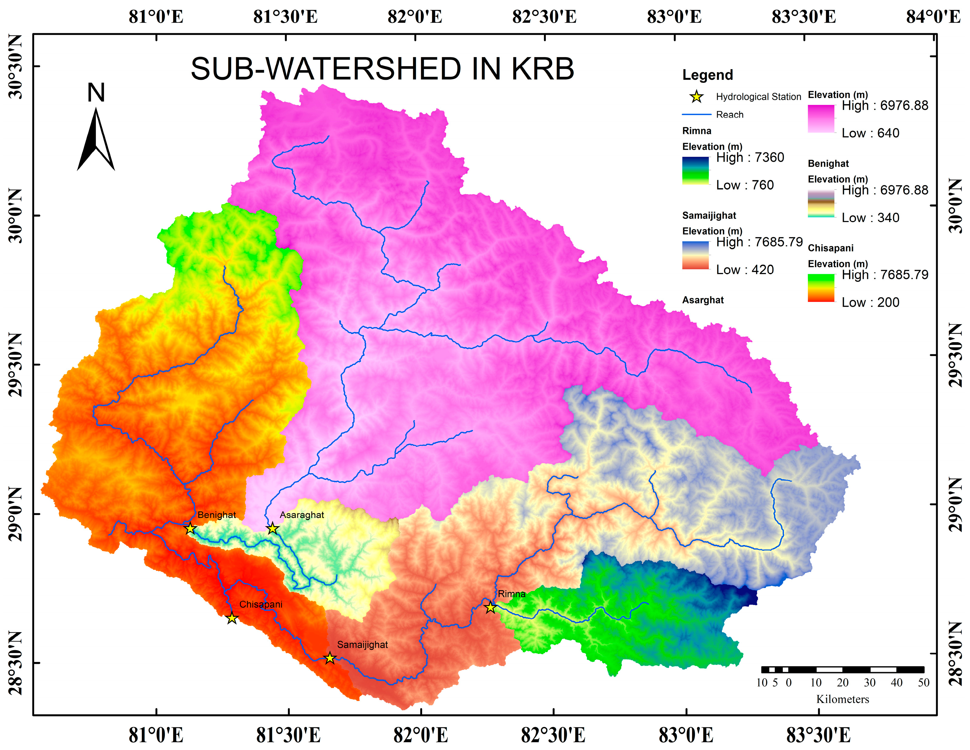
Figure 5.
This map illustrates the KRB area, delineating five sub-watersheds with their corresponding hydrological stations: Karnali River at Asaraghat (Q240), Karnali River at Benighat (Q250), Thulo Bheri River at Rimna (Q265), Bheri River at Samaijighat (Q269.5), and Karnali River at Chisapani (Q280). The delineation includes elevation ranges and the river network for each sub-watershed, providing a comprehensive geographical overview.
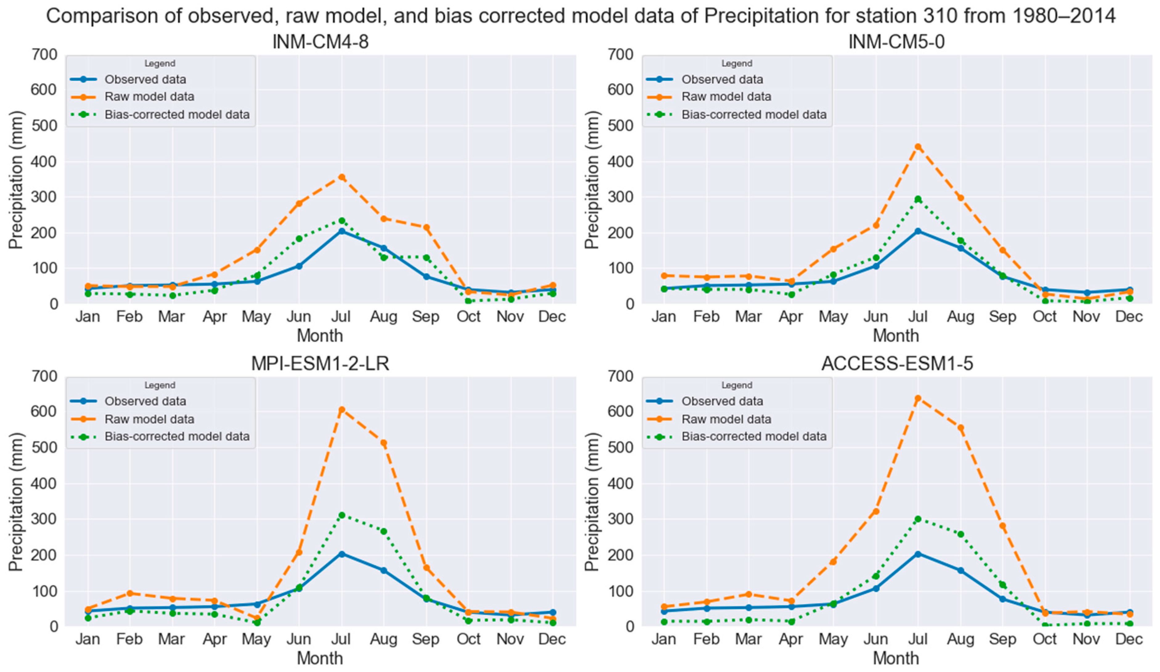
Figure 6.
Graph comparing observed with raw model, and bias-corrected average monthly precipitation during 1980 to 2014 for four selected GCCMs (INM-CM4-8, INM-CM5-0, MPI-ESM1-2-LR, and ACCESS-ESM1-5) for the hilly region of station 310.
Figure 6.
Graph comparing observed with raw model, and bias-corrected average monthly precipitation during 1980 to 2014 for four selected GCCMs (INM-CM4-8, INM-CM5-0, MPI-ESM1-2-LR, and ACCESS-ESM1-5) for the hilly region of station 310.
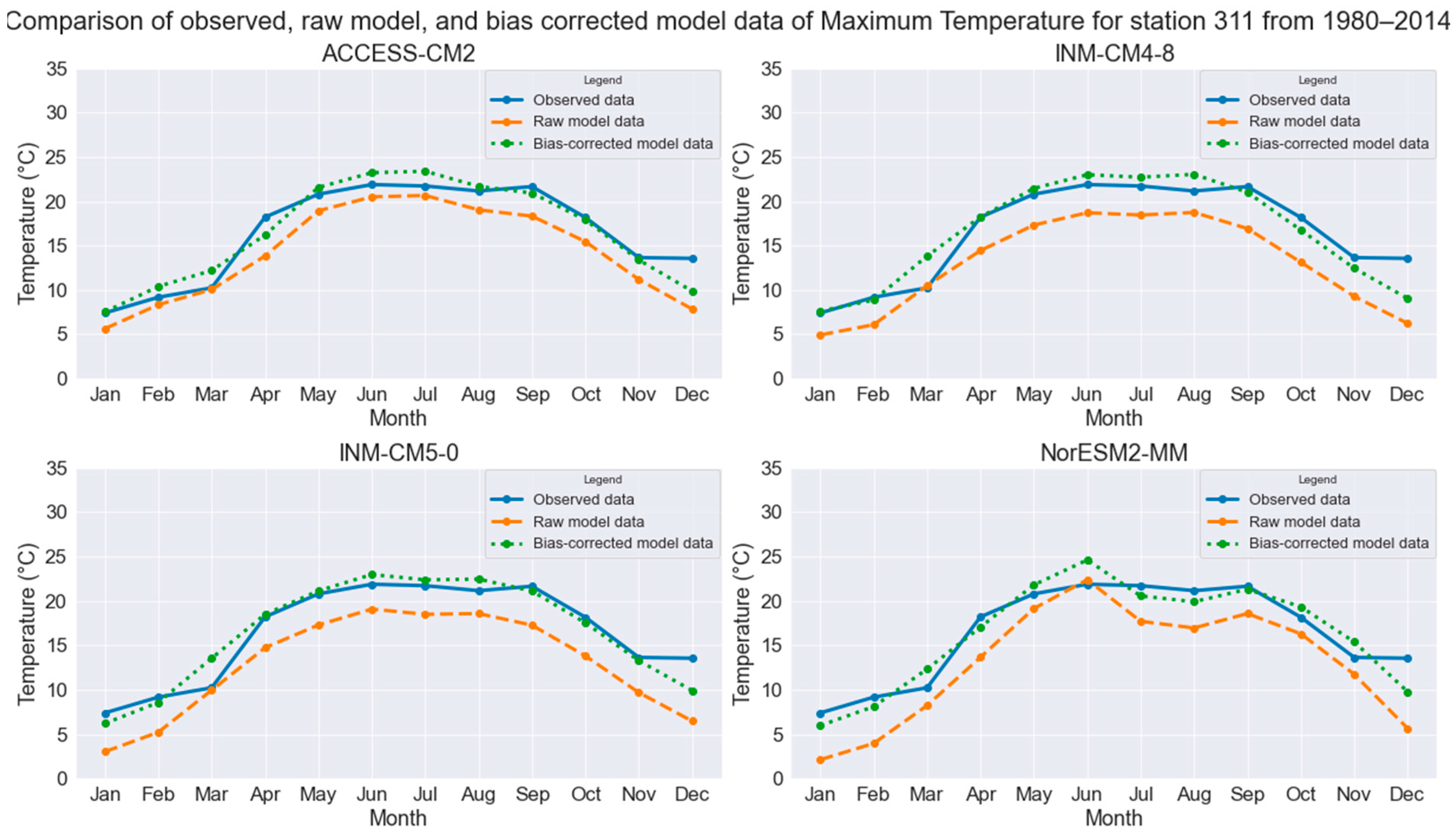
Figure 7.
Graph comparing observed with raw and bias-corrected average monthly maximum temperature during 1980 to 2014 for four selected GCCMs (ACCESS-CM2, INM-CM8-8, INM-CM5-0, and NorESM2-MM) for the mountainous region of station 311.
Figure 7.
Graph comparing observed with raw and bias-corrected average monthly maximum temperature during 1980 to 2014 for four selected GCCMs (ACCESS-CM2, INM-CM8-8, INM-CM5-0, and NorESM2-MM) for the mountainous region of station 311.
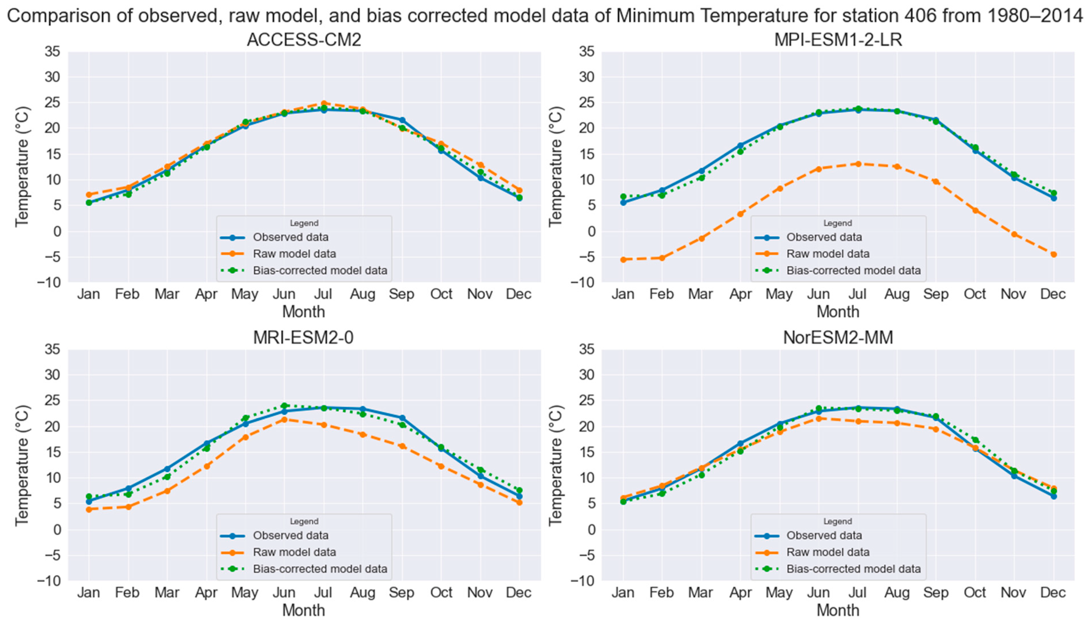
Figure 8.
Graph comparing observed with raw and bias-corrected average monthly minimum temperature during 1980 to 2014 for four selected GCCMs (ACCESS-CM2, MPI-ESM2-LR, MRI-ESM2-0, and NorESM2-MM) for the plains region of station 406.
Figure 8.
Graph comparing observed with raw and bias-corrected average monthly minimum temperature during 1980 to 2014 for four selected GCCMs (ACCESS-CM2, MPI-ESM2-LR, MRI-ESM2-0, and NorESM2-MM) for the plains region of station 406.
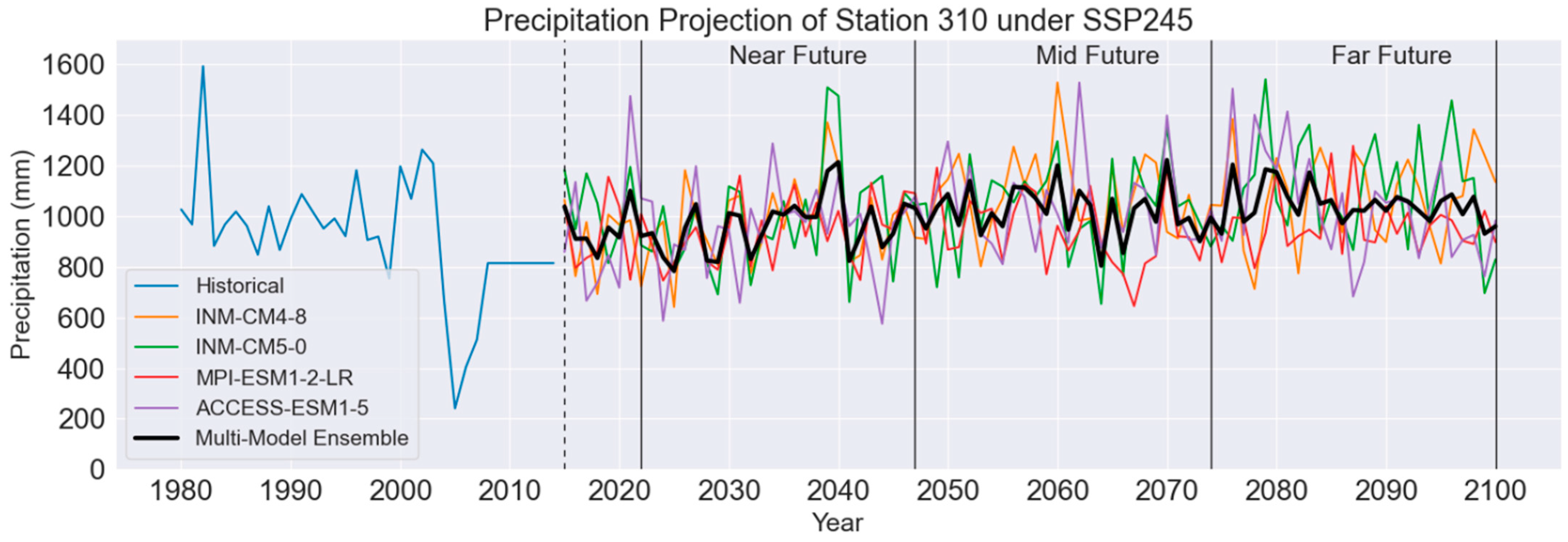
Figure 9.
Average annual precipitation trends at the hilly region station (310), detailing historical records and future projections under the SSP245 scenario from four selected GCMs alongside a Multi-Model Ensemble (MME) synthesis.
Figure 9.
Average annual precipitation trends at the hilly region station (310), detailing historical records and future projections under the SSP245 scenario from four selected GCMs alongside a Multi-Model Ensemble (MME) synthesis.
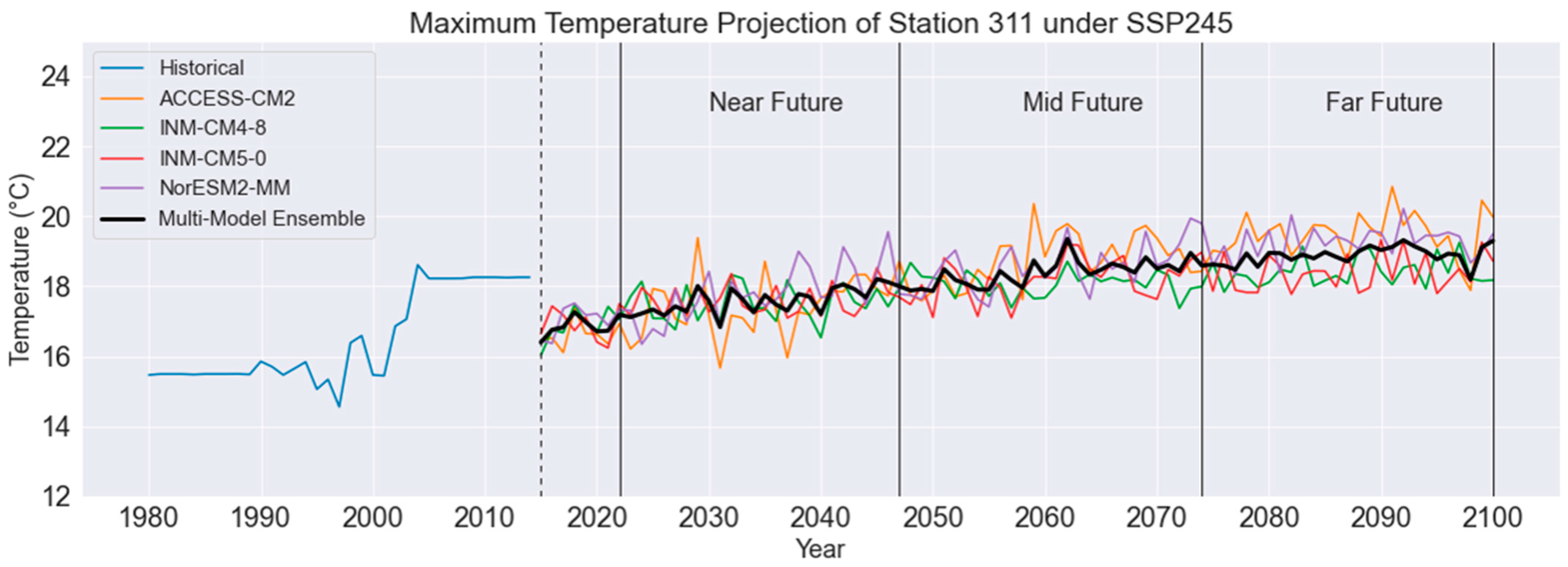
Figure 10.
Average annual maximum temperature trends at the mountainous region station (311), detailing historical records and future projections under the SSP245 scenario from four selected GCMs alongside a Multi-Model Ensemble (MME) synthesis.
Figure 10.
Average annual maximum temperature trends at the mountainous region station (311), detailing historical records and future projections under the SSP245 scenario from four selected GCMs alongside a Multi-Model Ensemble (MME) synthesis.
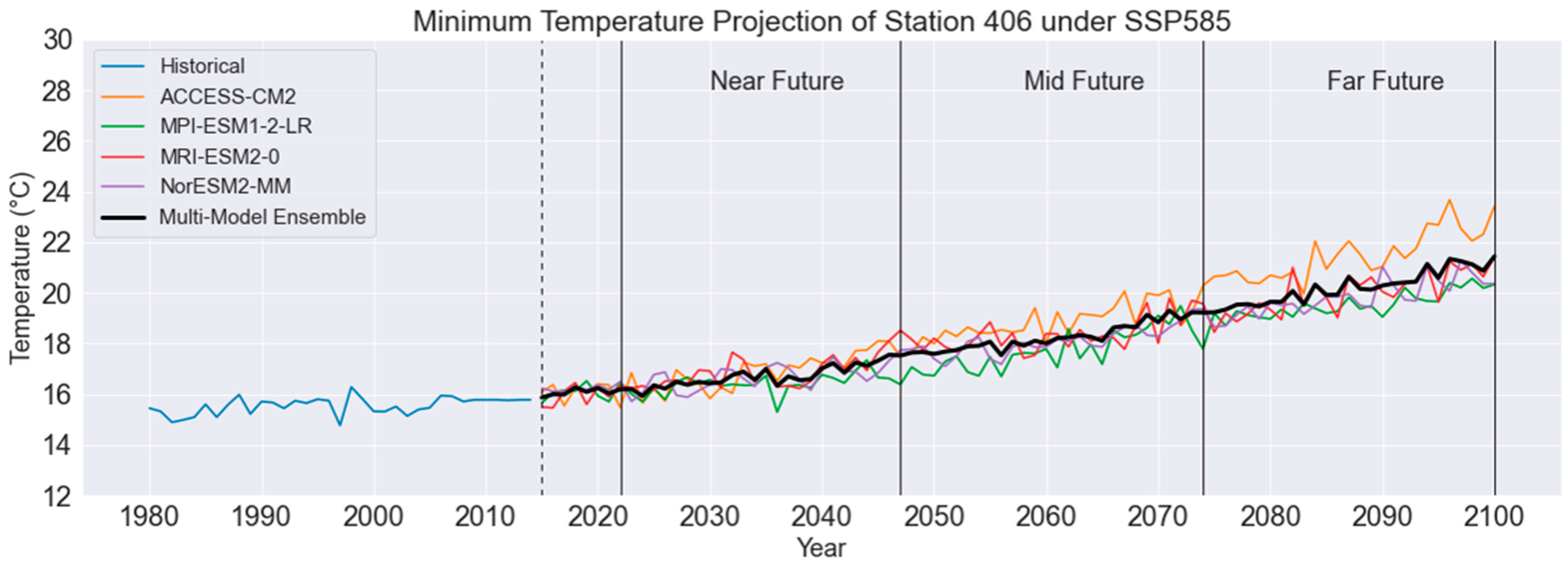
Figure 11.
Average annual minimum temperature trends at the plains region station (406), detailing historical records and future projections under the SSP245 scenario from four selected GCMs alongside a Multi-Model Ensemble (MME) synthesis.
Figure 11.
Average annual minimum temperature trends at the plains region station (406), detailing historical records and future projections under the SSP245 scenario from four selected GCMs alongside a Multi-Model Ensemble (MME) synthesis.
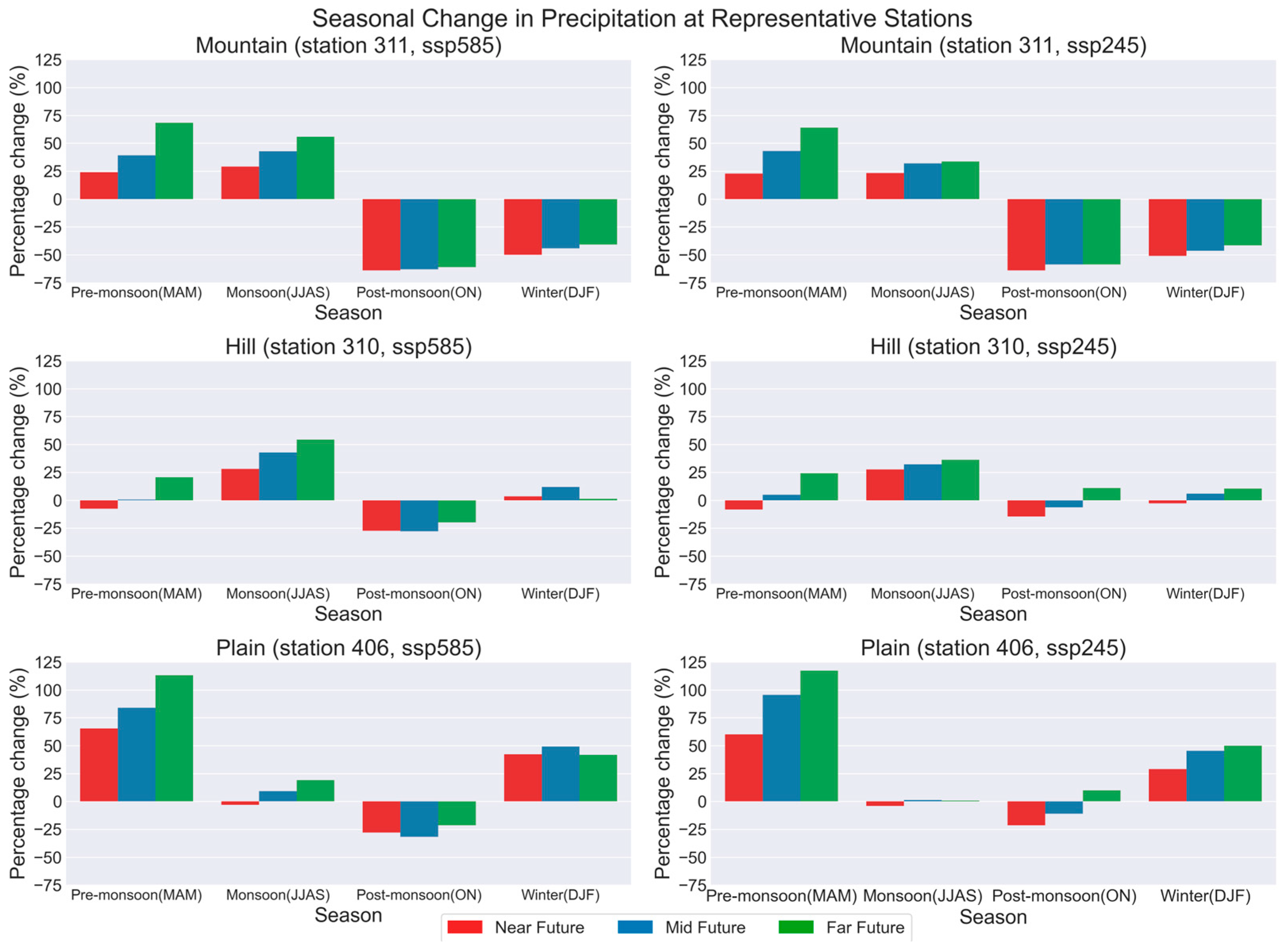
Figure 12.
Seasonal changes in precipitation at three representative (mountain, hilly, and plains) stations across the KRB under the SSP245 and SSP585 scenarios.
Figure 12.
Seasonal changes in precipitation at three representative (mountain, hilly, and plains) stations across the KRB under the SSP245 and SSP585 scenarios.
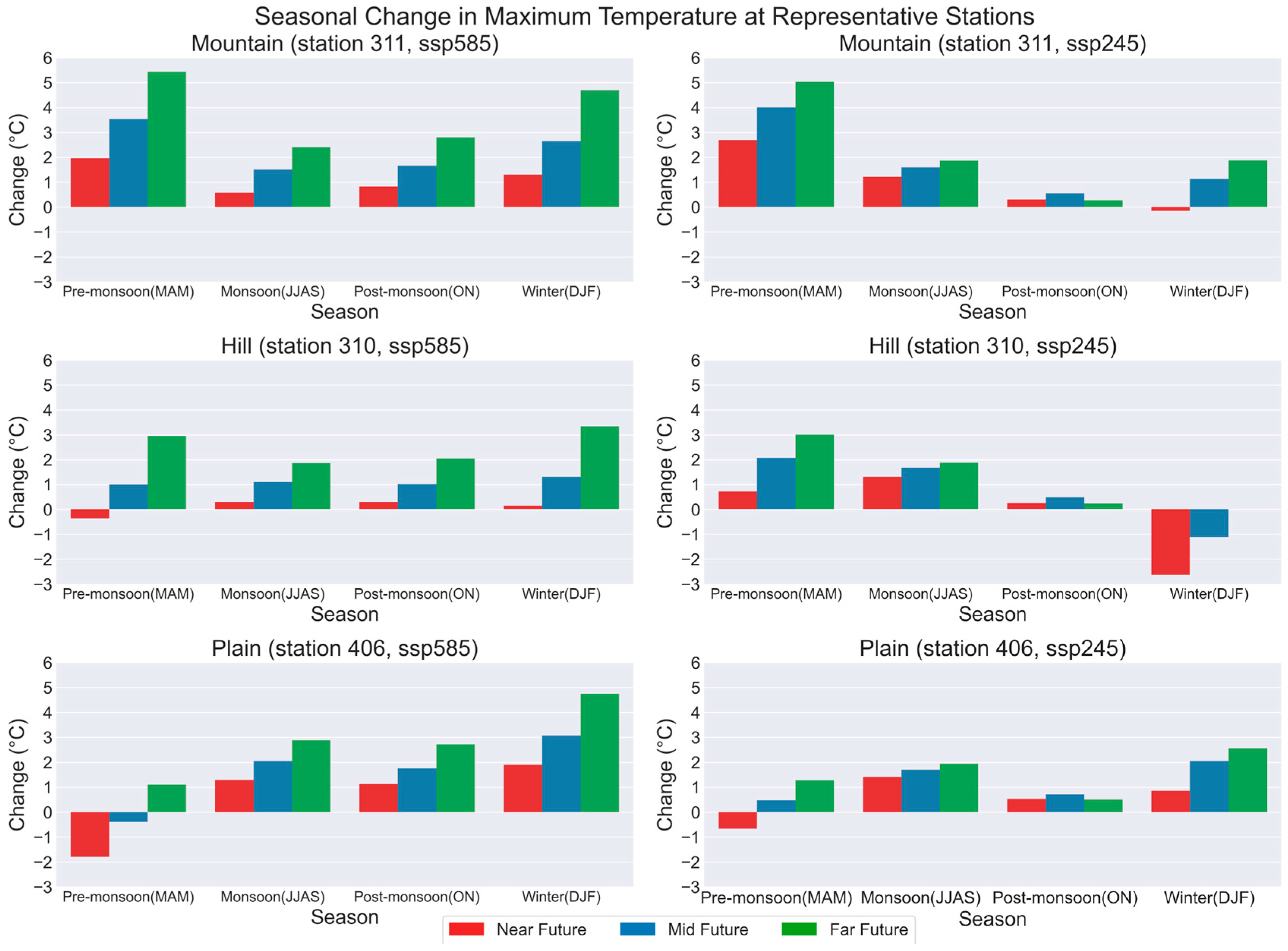
Figure 13.
Seasonal changes in maximum temperature at three representative (mountain, hilly, and plains) stations across the KRB under SSP245 and SSP585 scenarios.
Figure 13.
Seasonal changes in maximum temperature at three representative (mountain, hilly, and plains) stations across the KRB under SSP245 and SSP585 scenarios.
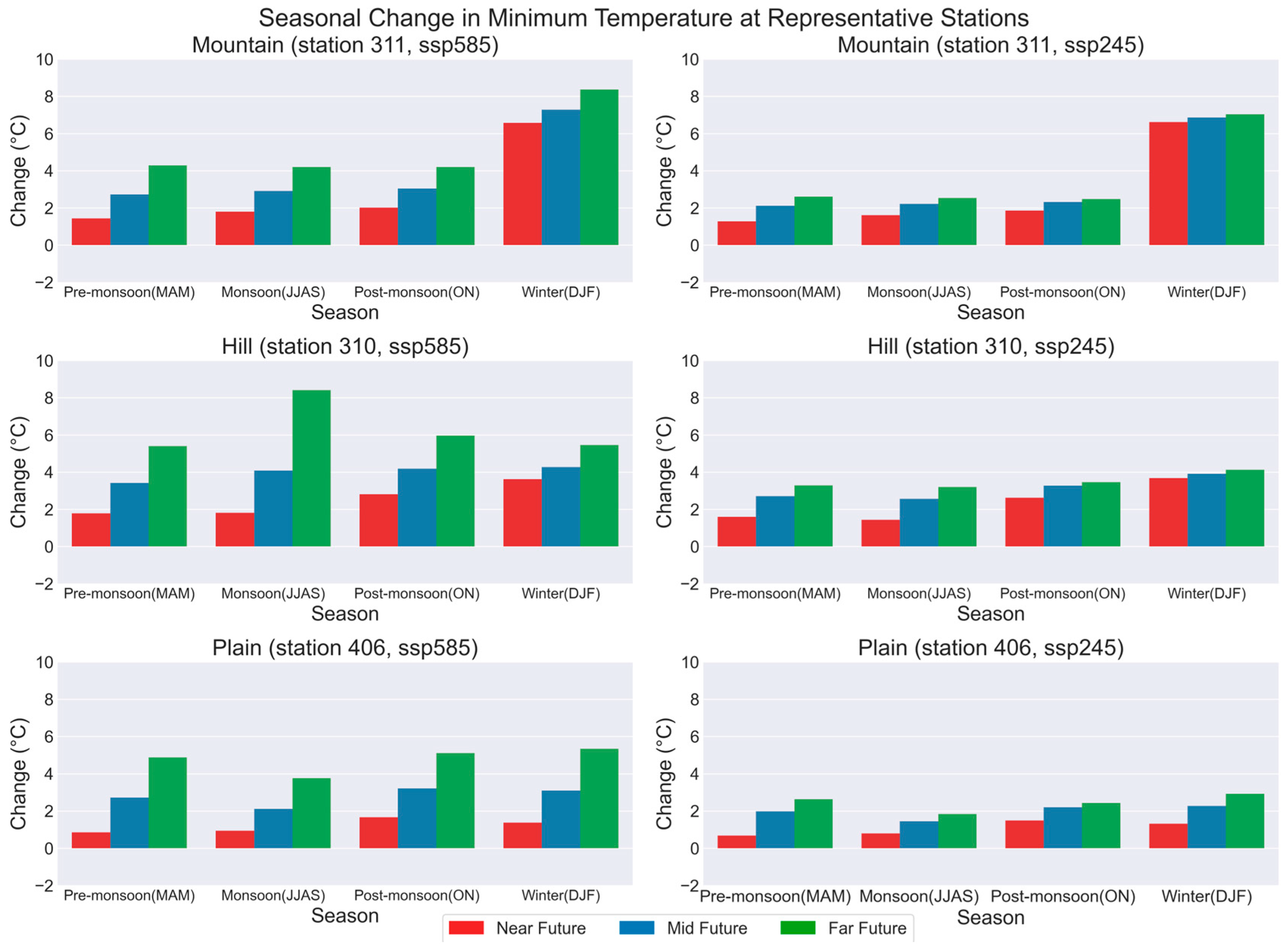
Figure 14.
Seasonal changes in minimum temperature at three representative (mountain, hilly, and plains) stations across the KRB under SSP245 and SSP585 scenarios.
Figure 14.
Seasonal changes in minimum temperature at three representative (mountain, hilly, and plains) stations across the KRB under SSP245 and SSP585 scenarios.
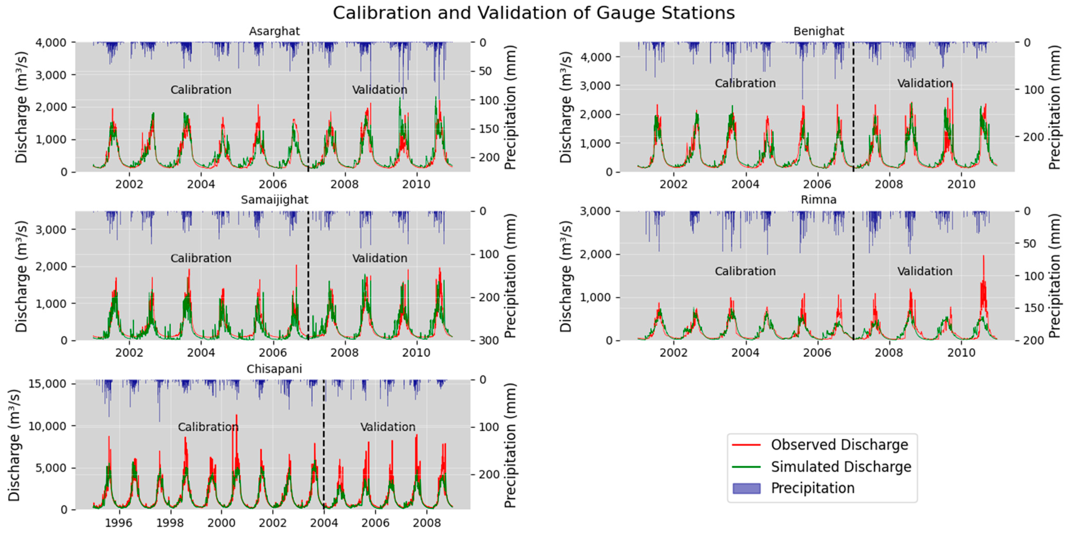
Figure 15.
Comparison of simulated and observed flow at five gauge stations across the KRB, namely the Karnali River at Asaraghat (Q240), Karnali River at Benighat (Q250), Thulo Bheri River at Rimna (Q265), Bheri River at Samaijighat (Q269.5), and Karnali River at Chisapani (Q280).
Figure 15.
Comparison of simulated and observed flow at five gauge stations across the KRB, namely the Karnali River at Asaraghat (Q240), Karnali River at Benighat (Q250), Thulo Bheri River at Rimna (Q265), Bheri River at Samaijighat (Q269.5), and Karnali River at Chisapani (Q280).
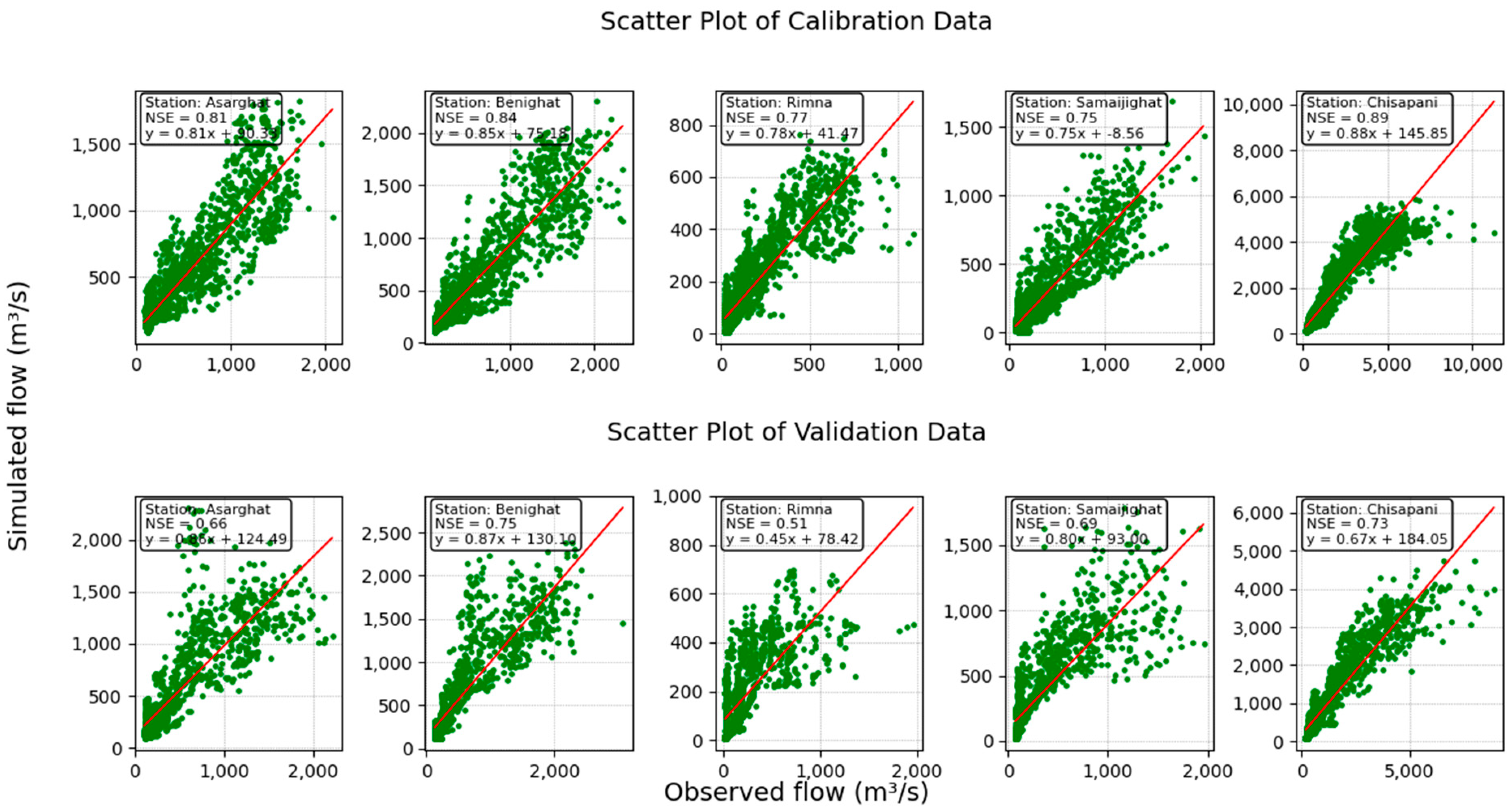
Figure 16.
Scatter plot between observed and simulated discharge at five gauge stations across the KRB, namely the Karnali River at Asaraghat (Q240), Karnali River at Benighat (Q250), Thulo Bheri River at Rimna (Q265), Bheri River at Samaijighat (Q269.5), and Karnali River at Chisapani (Q280).
Figure 16.
Scatter plot between observed and simulated discharge at five gauge stations across the KRB, namely the Karnali River at Asaraghat (Q240), Karnali River at Benighat (Q250), Thulo Bheri River at Rimna (Q265), Bheri River at Samaijighat (Q269.5), and Karnali River at Chisapani (Q280).
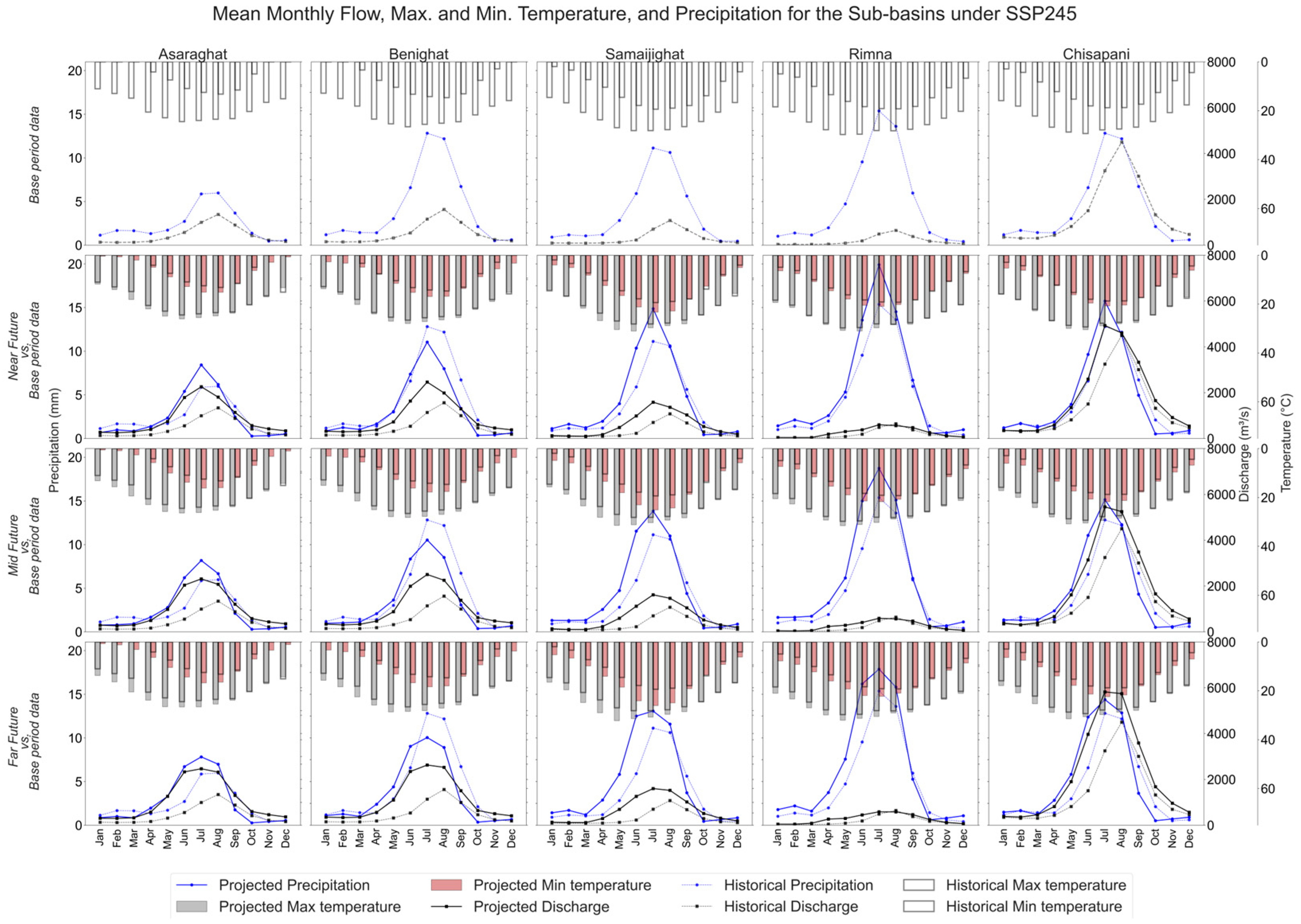
Figure 17.
Comparison of the average monthly observed discharge with projected discharge, maximum temperature, minimum temperature, and precipitation at five gauge stations within the KRB, analyzed under the SSP245 scenario across three future timeframes (NN, MF, and FF).
Figure 17.
Comparison of the average monthly observed discharge with projected discharge, maximum temperature, minimum temperature, and precipitation at five gauge stations within the KRB, analyzed under the SSP245 scenario across three future timeframes (NN, MF, and FF).
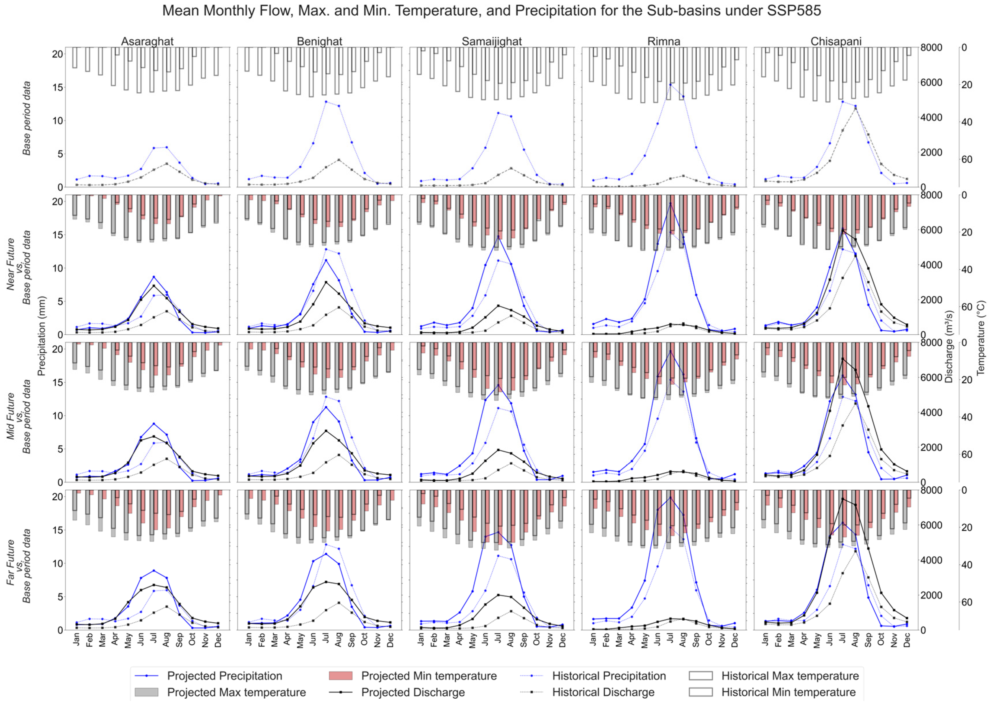
Figure 18.
Comparison of the average monthly observed discharge with projected discharge, maximum temperature, minimum temperature, and precipitation at five gauge stations within the KRB, analyzed under the SSP585 scenario across three future timeframes (NN, MF, and FF).
Figure 18.
Comparison of the average monthly observed discharge with projected discharge, maximum temperature, minimum temperature, and precipitation at five gauge stations within the KRB, analyzed under the SSP585 scenario across three future timeframes (NN, MF, and FF).
Table 1.
Meteorological station information.
Table 1.
Meteorological station information.
| SN | Station Name | Index No | District | Longitude
(°) | Latitude
(°) | Elevation
(m) | Annual
Precipitation (mm) | Annual Max. Temperature (°C) | Annual Min. Temperature (°C) |
|---|
| 1 | Dadeldhura | 104 | Dadeldhura | 80.58 | 29.30 | 1879 | - | 33.2 | −5 |
| 2 | Pipalkot | 201 | Bajhang | 80.84 | 29.61 | 1455 | 2133.7 | - | - |
| 3 | Silgsdhi | 203 | Doti | 80.98 | 29.26 | 1309 | - | 39 | −0.5 |
| 4 | Martadi | 204 | Bajura | 81.48 | 29.45 | 1598 | 2220.6 | - | - |
| 5 | Kola Gauna | 214 | Doti | 80.70 | 29.12 | 1364 | 2316.6 | - | - |
| 6 | Mangalsen | 217 | Achham | 81.25 | 29.13 | 1310 | 1598.8 | - | - |
| 7 | Rara | 307 | Mugu | 82.08 | 29.54 | 2989 | 834.2 | - | - |
| 8 | Dipal Gaun | 310 | Jumla | 82.22 | 29.26 | 2422 | 919.2 | 34.9 | −14 |
| 9 | Simikot | 311 | Humla | 81.81 | 29.97 | 2993 | 828.6 | 29.5 | −17.5 |
| 10 | Dunai | 312 | Dolpa | 82.89 | 28.95 | 2098 | 375.9 | 36.3 | −7 |
| 11 | Pusma Camp | 401 | Surkhet | 81.23 | 28.87 | 953 | 1738.1 | 39 | 0 |
| 12 | Dailekh | 402 | Dailekh | 81.70 | 28.83 | 1394 | 1958.6 | 39.6 | 0 |
| 13 | Birendra Nagar | 406 | Surkhet | 81.63 | 28.58 | 720 | 1737.6 | 41.8 | 0.5 |
| 14 | Maina Gaun | 418 | Mugu | 82.26 | 28.96 | 1913 | 1908.4 | - | - |
| 15 | Rukumkot | 501 | Rukum | 82.62 | 28.61 | 1568 | 1754.3 | - | - |
| 16 | Chaurjhari Tar | 513 | Rukum | 82.21 | 28.65 | 863 | 1259.3 | 42 | 0.5 |
| 17 | Musikot | 514 | Rukum | 82.46 | 28.61 | 1412 | - | 41.9 | −0.5 |
Table 2.
Information on CMIP6 models used in this study, including model name, institutions, and atmospheric resolution.
Table 2.
Information on CMIP6 models used in this study, including model name, institutions, and atmospheric resolution.
| SN | Model | Institution | Resolution |
|---|
| 1 | ACCESS-CM2 | Commonwealth Scientific and Industrial Research Organisation (CSIRO) and ACCESS (Australian Research Council Centre of Excellence for Climate System Science. | 1.25° × 1.875° |
| 2 | ACCESS-ESMI | Commonwealth Scientific and Industrial Research Organisation (CSIRO) and ACCESS (Australian Research Council Centre of Excellence for Climate System Science | 1.25° × 1.875° |
| 3 | BCC-CSM2-MR | Beijing Climate Center, Beijing | 1.125° × 1.125° |
| 4 | EC-Earth3 | EC-Earth Consortium | 0.35° × 0.35° |
| 5 | FGOALS-f3-L | Chinese Academy of Sciences Flexible Global Ocean–Atmosphere–Land System model | 1° × 1° |
| 6 | INM-CM4-8 | Institute for Numerical Mathematics, Russia | 2° × 1.5° |
| 7 | IPSL-CM6A-LR | Institute Pierre Simon Laplace (IPSL), Paris | 2.5° × 1.27° |
| 8 | INM.INM-CM4-8 | Institute for Numerical Mathematics, Russia | 2° × 1.5° |
| 9 | INM-CM5-0 | Institute for Numerical Mathematics, Russia | 2° × 1.5° |
| 10 | MPI-ESM1-2-HR | Max Planck Institute for Meteorology (MPI-M), Germany | 0.94° × 0.94° |
| 11 | MRI-ESM2-0 | Meteorological Research Institute, Ibaraki, Japan | 1.125° × 1.125° |
| 12 | MPI-ESM1-2-LR | Max Planck Institute for Meteorology (MPI-M), Germany | 1.875° × 1.86° |
| 13 | MIROC6 | Japan Agency for Marine-Earth Science and Technology (JAMSTEC), Kanagawa | 1.4° × 1.4° |
| 14 | NorESM2-MM | Norwegian Climate Center, Norway | 2.5° × 1.89° |
Table 3.
Rating system of performance metrics [
37].
Table 3.
Rating system of performance metrics [
37].
| Rating | NSR | RSR | PBIAS | R2 | Ratings |
|---|
| Very Good | 0.75–1.00 | 0.00–0.50 | <10 | 75–100 | 5 |
| Good | 0.55–0.75 | 0.50–0.6 | 15-Oct | 65–75 | 4 |
| Satisfactory | 0.40–0.55 | 0.60–0.70 | 15–25 | 50–65 | 3 |
| Unsatisfactory | 0.25–0.40 | 0.70–0.80 | 25–35 | 40–50 | 2 |
| Poor | ≤0.25 | >0.80 | ≥35 | <40 | 1 |
Table 4.
Sub-basin number, HRU number, calibration, and validation period for different gauge stations.
Table 4.
Sub-basin number, HRU number, calibration, and validation period for different gauge stations.
| Watershed | Sub-Watershed | Area (km2) | No. of Sub-Basin | No. of HRUs | Warm-Up Period (yrs) | Calibration Period | Validation Period |
|---|
| KRB | Rimna | 2712.70 | 1 | 7 | 2 | 2001–2006 | 2007–2010 |
| Samaijighat | 12,615.75 | 11 | 66 | 2 | 2001–2006 | 2007–2010 |
| Benighat | 19,467.94 | 21 | 120 | 2 | 2001–2006 | 2007–2010 |
| Asaraghat | 17,668.20 | 18 | 108 | 2 | 2001–2006 | 2007–2010 |
| Chisapani | 42,086.67 | 45 | 248 | 2 | 1995–2003 | 2004–2008 |
Table 5.
Performance rating of CMIP6 GCMs.
Table 5.
Performance rating of CMIP6 GCMs.
| Precipitation | Rating | Max Temperature | Rating | Min Temperature | Rating |
|---|
| INM-CM5-0 | 2.464 | MPI-ESM1-2-HR | 3.050 | MPI-ESM1-2-HR | 3.575 |
| INM-CM4-8 | 2.446 | ACCESS-CM2 | 2.700 | NorESM2-MM | 3.475 |
| MPI-ESMI-2-LR | 2.339 | NorESM2-MM | 2.650 | ACCESS-CM2 | 3.300 |
| ACCESS-ESM1-5 | 2.321 | FGOALS-g3 | 2.550 | MRI-ESM2-0 | 3.300 |
| BCC-CSM2-MR | 2.196 | INM-CM4-8 | 2.475 | FGOALS-f3-L | 3.025 |
| MIROC6 | 2.125 | INM-CM5-0 | 2.350 | MPI-ESM1-2-LR | 2.750 |
| NorESM2-MM | 1.875 | BCC-CSM2-MR | 2.350 | INM-CM4-8 | 2.550 |
| ACCESS-CM2 | 1.214 | IPSL-CM6A-LR | 2.125 | INM-CM5-0 | 2.500 |
| MRI-ESM2-0 | 1.214 | MRI-ESM2-0 | 2.125 | EC-Earth3 | 2.325 |
| | | EC-Earth3 | 1.000 | IPSL-CM6A-LR | 2.250 |
Table 6.
Performance rating of the bias correction methods.
Table 6.
Performance rating of the bias correction methods.
| Bias Correction Methods | Rating |
|---|
| Precipitation | Maximum Temperature | Minimum Temperature |
|---|
| Bernoulli Exponential | 1.90 | | |
| Bernoulli Gamma | 2.43 | | |
| Bernoulli Weibull | 2.56 | | |
| Bernoulli Log-normal | 2.01 | | |
| Non-parametric quantile mapping using empirical quantiles—linear | 2.02 | 3.68 | 4.06 |
| Non-parametric quantile mapping using empirical quantiles—tricub | 2.08 | 3.71 | 4.06 |
| Parameter Transformation function—exponential asymptote | 1.72 | 4.33 | 4.01 |
| Parameter Transformation function—linear | 2.24 | 4.37 | 4.07 |
| Parameter Transformation function—power | 2.27 | 3.10 | 3.14 |
| Parameter Transformation function—scale | 1.56 | 3.96 | 3.43 |
| Non-parametric quantile mapping using robust empirical quantiles—linear | 2.05 | 3.68 | 4.06 |
| Non-parametric quantile mapping using robust empirical quantiles—tricub | 2.10 | 3.75 | 4.09 |
| Quantile mapping using a smoothing spline | 2.24 | 4.168 | 4.20 |
Table 7.
Net change in projected precipitation, maximum temperature, and minimum temperature at station-310, -311, and -406 and an average for all stations (All).
Table 7.
Net change in projected precipitation, maximum temperature, and minimum temperature at station-310, -311, and -406 and an average for all stations (All).
| SSP245 | Precipitation (%) | Maximum Temperature (°C/yr) | Minimum Temperature (°C/yr) |
|---|
| Stations | NF | MF | FF | NF | MF | FF | NF | MF | FF |
|---|
| 310 | +4.73 | +11.21 | +13.72 | +0.0003 | +0.032 | +0.054 | +0.086 | +0.117 | +0.134 |
| 311 | +1.67 | +10.61 | +14.47 | +0.042 | +0.073 | +0.091 | +0.107 | +0.128 | +0.14 |
| 406 | −2.19 | +5.05 | +7.58 | +0.0001 | +0.027 | +0.041 | +0.039 | +0.073 | +0.092 |
| All | +7.79 | +11.65 | +16.25 | +0.018 | +0.048 | +0.064 | +0.049 | +0.08 | +0.097 |
| SSP585 | Precipitation (%) | Maximum Temperature (°C/yr) | Minimum Temperature (°C/yr) |
| Stations | NF | MF | FF | NF | MF | FF | NF | MF | FF |
| 310 | +6.48 | +13.49 | +24.17 | +0.003 | +0.041 | +0.097 | +0.09 | +0.153 | +0.25 |
| 311 | +6.12 | +15.94 | +28.78 | +0.044 | +0.088 | +0.144 | +0.112 | +0.152 | +0.201 |
| 406 | +0.69 | +8.41 | +20.75 | +0.024 | +0.062 | +0.109 | +0.044 | +0.103 | +0.178 |
| All | +9.43 | +16.51 | +27.47 | +0.022 | +0.066 | +0.119 | +0.057 | +0.115 | +0.187 |
Table 8.
Calibrated values of the SWAT parameters for the hydrological stations.
Table 8.
Calibrated values of the SWAT parameters for the hydrological stations.
| Parameter | Change Type | Suggested Ranges | | | Gauge Stations | | |
|---|
| Asaraghat | Benighat | Rimna | Samaijighat | Chisapani |
|---|
| CN2 | r | 35–98 | 60.2 | 58.9 | 50.7 | 53.9 | 53.3 |
| ALPHA_BF | v | 0–1 | 0.12 | 0.31 | 0.28 | 0.19 | 0.23 |
| GW_DELAY | v | 0–500 | 189.11 | 152.68 | 42.87 | 57.56 | 51.39 |
| GWQMN | v | 0–5000 | 1.41 | 1.39 | 1.28 | 1.39 | 1.3 |
| GW_REVAP | v | 0.02–0.2 | 0.03 | −0.02 | 0.04 | 0.13 | 0.04 |
| ESCO | v | 0–1 | 0.87 | 0.84 | 0.86 | 0.88 | 0.84 |
| CH_N2 | v | −0.01–0.3 | 0.29 | 0.29 | 0.32 | 0.32 | 0.32 |
| CH_K2 | v | −0.01–500 | 86.52 | 94.98 | 75.19 | 75.51 | 65.71 |
| ALPHA_BNK | v | 0–1 | 0.56 | 0.63 | 0.5 | 0.52 | 0.57 |
| SOL_AWC | r | 0–1 | 0.5 | 0.51 | 0.52 | 0.58 | 0.51 |
| SOL_K | r | 0–2000 | 0.19 | 0.28 | 0.09 | 0.11 | 0.29 |
| SOL_BD | r | 0.9–2.5 | −1.56 | −1.17 | −1.48 | −1.12 | −1.01 |
| HRU_SLP | r | 0–1 | 0.25 | 0.23 | 0.24 | 0.31 | 0.31 |
| OV_N | r | 0.01–1 | 1.02 | 1.06 | 1 | 0.99 | 1.07 |
| SLSUBBSN | r | 10–150 | 72.79 | 65.32 | 62.6 | 68.57 | 70.9 |
| REVAPMN | v | 0–500 | 661.4 | 693.56 | 737.55 | 678.21 | 692.21 |
| RCHRG_DP | a | 0–1 | −0.08 | −0.06 | −0.15 | −0.09 | −0.06 |
| SHALLST | r | 0–50,000 | 30,916.34 | 28,810.26 | 25,901.14 | 18,576.11 | 33,973.12 |
| CANMX | r | 0–100 | 86.71 | 90.27 | 80.96 | 81.07 | 94.55 |
| EPCO | r | 0–1 | 0.76 | 0.76 | 0.7 | 0.71 | 0.71 |
| LAT_TTIME | r | 0–180 | −1.13 | −0.5 | 25.81 | −78.45 | −21.28 |
| CH_N1 | r | 0.01–30 | 4.28 | 10.62 | 5.19 | 1.84 | −2.92 |
| SFTMP | v | −20–20 | 0.57 | 2.42 | - | 0.42 | 1.06 |
| SMTMP | v | −20–20 | 2.93 | 1.83 | - | 3.39 | 2.06 |
| SMFMX | v | 0–20 | 4.85 | 6.87 | - | 8.52 | 6.07 |
| SMFMN | v | 0–20 | 3.5 | 0.75 | - | 0.52 | 0.86 |
| TIMP | v | 0–1 | 0.08 | 0.02 | - | −0.32 | −0.3 |
| PLAPS | v | −1000–1000 | 0.02 | 0.02 | 0.05 | 0.02 | 0.02 |
| TLAPS | v | −10–10 | −6.77 | −6.42 | −7.14 | −7.86 | −8.09 |
| SURLAG | v | 0.05–24 | - | - | - | 2.4 | 2.41 |
Table 9.
Performance of calibration and validation.
Table 9.
Performance of calibration and validation.
| Station | Variable Period | NSE | R2 | PBIAS |
|---|
| Asaraghat | Calibration period (2001–2006) | 0.81 | 0.81 | −0.7 |
| Validation period (2007–2010) | 0.66 | 0.71 | −12.5 |
| Benighat | Calibration period (2001–2006) | 0.84 | 0.84 | −0.1 |
| Validation period (2007–2010) | 0.75 | 0.78 | −12.1 |
| Rimna | Calibration period (2001–2006) | 0.77 | 0.77 | −0.6 |
| Validation period (2007–2010) | 0.51 | 0.54 | 16.1 |
| Samaijighat | Calibration period (2001–2006) | 0.75 | 0.82 | 28.1 |
| Validation period (2007–2010) | 0.69 | 0.71 | −9.6 |
| Chisapani | Calibration period (1995–2003) | 0.89 | 0.89 | 1.9 |
| Validation period (2004–2008) | 0.73 | 0.74 | −5.7 |

 ,
, 


