Article

Optimal Vehicle Scheduling and Charging Infrastructure Planning for Autonomous Modular Transit System

1
College of Forensic Sciences, Criminal Investigation Police University of China, Shenyang 110035, China
2
School of Transportation, Jilin University, Changchun 130022, China
3
State Key Laboratory for Strength and Vibration of Mechanical Structures, School of Aerospace Engineering, Xi’an Jiaotong University, Xi’an 710049, China
*
Authors to whom correspondence should be addressed.
Sustainability 2024, 16(8), 3316; https://doi.org/10.3390/su16083316
Submission received: 24 January 2024 / Revised: 21 March 2024 / Accepted: 9 April 2024 / Published: 16 April 2024
(This article belongs to the Section Sustainable Transportation)

Abstract

:
Prioritizing the development of public transport is an effective way to improve the sustainability of the transport system. In recent years, bus passenger flow has been declining in many cities. How to reform the operating mode of the public transportation system is an important issue that needs to be solved. An autonomous modular bus (AMB) is capable of physical coupling and uncoupling to flexibly adjust vehicle capacity as well as provide high-quality service under unbalanced passenger demand conditions. To promote AMB adoption and reduce the operating cost of the bus route, this paper presents a joint optimization method to simultaneously determine the AMB dispatching plan, charging plan, and charging infrastructure configuration scheme. Then, a mixed-integer programming model is formulated to minimize the operating costs of the bus route. A hybrid intelligent algorithm combining enumeration, cloning algorithm, and particle swarm optimization algorithm is designed to resolve the formulated model. Subsequently, an actual bus route is taken as an example to validate the proposed method. Results indicate that the developed method in this paper can reduce the operating costs and operational energy consumption of the route compared with the real route operating plan. Specifically, the reduction ratio of the former is 23.85%, and the reduction ratio of the latter is 5.92%. The results of this study validate the feasibility and advantages of autonomous modular transit service, contributing positively to the sustainable development of the urban public transportation system.

1. Introduction

Prioritizing the promotion of public transportation is a proven way to reduce emissions from transport and improve the sustainability of society [1,2]. Recently, bus passenger flow has continued to decline in many cities. How to reform the operating mode of the public transportation system to improve the travel efficiency of passengers and reduce the operating costs of bus companies has become a vital issue for the current public transportation system. Nowadays, an emerging approach to urban public transportation, autonomous modular buses (AMBs), has attracted much attention [3,4]. The AMBs are electrically powered buses equipped with autonomous driving capabilities, which can operate independently on a specific route and physically couple and uncouple as operationally needed. This means that the spatiotemporal heterogeneity of passenger demand can be solved by adjusting the number of AMBs performing different trips [5,6,7]. Furthermore, it is permissible to specify which vehicle provides energy during the trip when several AMBs are coupled to perform a trip together. Generally, only the first vehicle of the coupled AMBs provides energy, and no energy is consumed by other vehicles. In such a case, when the first AMB has insufficient electricity, a group of AMBs can continue to perform a trip by replacing the first AMB with the other one of the residual AMBs. During operation, the AMB with insufficient electricity can also return to the charging station for recharging individually. To sum up, AMBs can provide higher quality transit services at lower energy consumption and operating costs by adjusting vehicle capacity to change their service supply. The adoption of AMBs will significantly decrease environmental pollution, thus promoting the realization of a sustainable urban public transportation system.
From the above description, it is clear that the AMB dispatching problem not only involves assigning the trips in the timetable to the vehicles, but also arranging the order of AMBs that perform the same trip. Therefore, the dispatching methods for conventional fuel buses and electric buses are not suitable to be implemented in AMBs. The formulation for the AMB dispatching plan and charging plan is more complicated. On the one hand, due to the size constraints, the battery capacity of the AMB is limited and the battery needs to be recharged frequently during the daytime. On the other hand, which vehicle provides energy during the trip determines the state of charge (SOC) of each vehicle when several AMBs are connected together, and subsequently affects the AMB dispatching plan and charging plan. In addition, charging infrastructure configuration schemes also interact with the AMB dispatching plan and charging plan. Considering any of these problems individually may result in a sub-optimal transit system operating scheme [8]. Therefore, the integrated optimization of the AMB dispatching plan, charging plan, and charging infrastructure configuration plan is of great significance for a better transit system operation, and achieves the goals of reducing the operation costs of the modular transit network system (MTNS) and improving the theory of MTNS operation planning.
Hence, this study presents a collaborative optimization method to determine the AMB dispatching plan, charging plan, and charging infrastructure configuration plan. The main contributions of this study are as follows: (i) The SOC of the AMB is quantified under the condition that the first vehicle of the coupled AMBs provides energy during the entire trip. (ii) Considering the time-of-use tariff, we establish a nonlinear mixed-integer programming model that minimizes the operating costs. (iii) We use a combination of enumeration, cloning algorithm (CA), and particle swarm optimization (PSO) for designing a hybrid intelligent algorithm to solve the model and determine the AMB dispatching plan, charging plan, battery capacity, AMB fleet size, and number of chargers.
The structure of the paper is as follows: Section 2 reviews related literature discussing the integrated optimization of vehicle dispatching and charging infrastructure configuration and flexible capacity design for transit services. Section 3 describes the establishment process for the cooperative optimization model of AMB dispatching, charging scheduling, and charging infrastructure configuration and solution algorithm. Section 4 provides a case study on the basis of an actual bus route. Section 5 illustrates the research conclusions.

2. Literature Review

This study concentrates on the integrated optimization of vehicle dispatching and charging infrastructure configuration for the bus route operating AMB. Therefore, this paper discusses related work in terms of integrated optimization of vehicle dispatching and charging infrastructure configuration and flexible capacity design for transit services.

2.1. Integrated Optimization of Vehicle Dispatching and Charging Infrastructure Configuration

Recently, the EB transport planning process has become increasingly important as the electrification of urban public transport continues to advance [9,10,11,12,13]. Integrated planning for multi-problems increases the complexity and difficulty of solving the problem exponentially, compared with the step-by-step planning for a single problem. However, integrated planning can not only further decrease the transit system’s operational costs, but also enhance the transit service’s efficiency [14]. Hence, more and more researchers focus on the integrated optimization of two or more problems in the EB transport planning process, for instance, the integration of vehicle dispatching and charging infrastructure configuration [15,16]. Among them, charging infrastructure configuration includes the charging station location, number of chargers, battery capacity equipped in vehicles, etc. [17,18] Targeting the minimization of the overall operating costs, Wang et al. [19] and Hu et al. [20] collaboratively optimized the EB charging plan, number of chargers, and charging station location. Liu et al. [21] presented a collaborative optimization model for finding the optimal EB charging station location, number of chargers, charger power, and EB charging plan aimed at minimizing the costs of passengers’ waiting time and the EB system’s operating costs. McCabe et al. [22] presented an approach to concurrently determine the EB charger location, EB charging plan, and number of chargers by optimizing the tradeoff between the investment costs of charging facilities and operational performance. Aiming at minimizing total operational costs, He et al. [8] formulated a joint optimization model to determine the EB dispatching plan, EB charging plan, and charging infrastructure planning.
In addition, infrastructure configuration schemes interact with each other [23,24]. For instance, the number of chargers and the charging station location affect the EB charging plan, thus influencing the fleet size [25,26]. Aiming at minimizing the overall implementation costs, Ke et al. [27] established a model to find the optimal EB fleet size, number of chargers, and battery capacity. Liu et al. [28] formulated an optimal model to simultaneously determine the battery capacity and fast-charging station deployment plan under energy consumption uncertainty. He et al. [29] developed an EB fast-charging station deployment approach aimed at minimizing the electricity demand charges, battery acquisition costs, energy storage systems construction costs, and fast-charging stations construction costs. Alwesabi et al. [30] formulated a joint optimization model to concurrently determine the battery capacity and dynamic wireless charging facilities’ location. Considering integrated photovoltaic and energy storage systems, Liu et al. [31] presented a charging station planning model aimed at minimizing the charging infrastructure construction costs, charging costs, EB acquisition costs, and carbon emission costs.

2.2. Flexible Capacity Design for Transit Services

AMBs can be physically coupled or uncoupled as operationally required, thus enabling the provision of transit services with flexible capacity [3,32,33,34,35]. Chen et al. [36] and Chen et al. [37] determined the optimal departure frequency of AMBs and vehicle capacity under oversaturated traffic by employing discrete modeling and continuous modeling approaches, respectively. Shi et al. [38] concentrated on the collaborative optimization of the departure frequency and the length of AMB for each trip for shared corridors to minimize operating costs and passengers’ waiting time. Considering time-dependent travel demand, Ji et al. [6] presented a bi-objective (minimizing passengers’ waiting time and total empty seats of AMBs) optimization model to simultaneously determine the timetable, vehicle formation, and AMB dispatching plan. Aiming at minimizing the travel time costs of passengers and operational costs, Pei et al. [39] formulated a joint model to find the optimal vehicle capacity and headway in a modular transit network system (MTNS). Tian et al. [40] formulated a collaborative optimization model to concurrently determine the intermediate special stations’ location and capacity in an MTNS. Considering temporal dependencies on passenger demand and limited availability of the AMBs at stations, Tian et al. [41] established an AMB dispatching and vehicle formation integrated optimization model to minimize passengers’ waiting time costs, bus companies’ operating costs, and re-balancing costs of the AMBs. Khan et al. [4] designed a stop-skipping strategy leveraging physical coupling and uncoupling features of AMBs to minimize the passengers’ travel time. Aiming at minimizing the AMB system’s overall operating costs, Liu et al. [7] established a collaborative optimization model to find the optimal timetable, AMB dispatching plan, and vehicle formation. This model permitted the AMB to uncouple from one vehicle and couple to another vehicle in either direction on a bi-directional route. Guo et al. [42] applied AMBs to customized on-demand bus services and designed a two-phase method to determine the optimal AMB routing plan and charging plan.
The aforementioned studies have offered some suggestions for the operation and planning strategy of AMBs. However, the charging scheduling of AMBs was not considered in the aforementioned studies. There are significant differences in the development of a charging plan between AMBs and conventional electric buses. Investigating the charging scheduling of AMBs is imperative. Therefore, this paper proposes a collaborative optimization method for concurrently determining the AMB dispatching plan, charging plan, fleet size, number of chargers, and battery capacity, with the goal of minimizing operating costs.

3. Methodology

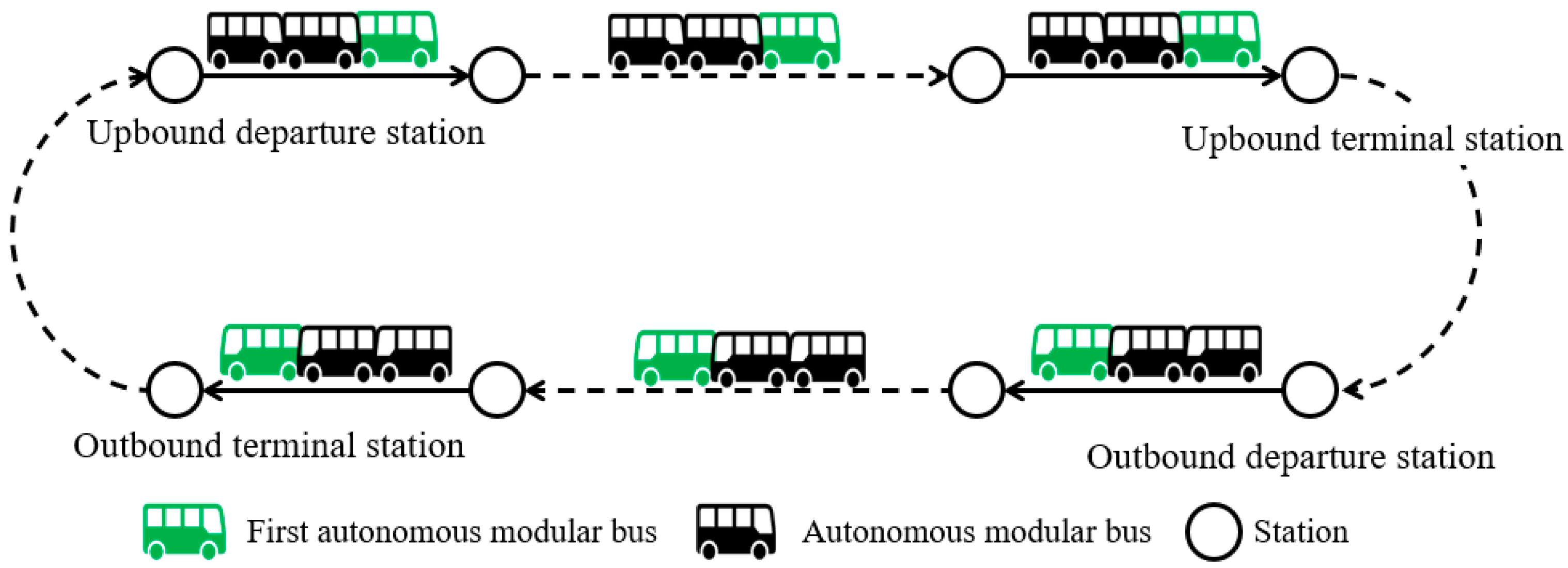
3.1. Problem Description

In this study, one trip refers to the process of an AMB departing from the upbound departure station of a route to the upbound terminal station (i.e., the outbound departure station) and back to the upbound departure station (i.e., the outbound terminal station). Let i   ( i = 1 ,   2 ,   ,   I ) represent the trip number on the route, where I is the total number of trips scheduled to operate every day. Let U represent the total number of AMBs deployed on the route and u   ( u = 1 ,   2 ,   ,   U ) denote the AMB number. Let B denote the battery capacity configured on AMBs. The charging station for AMBs is located at the upbound departure station on the route and is constructed with R chargers. Let r   ( r = 1 ,   2 ,   ,   R ) denote the charger number. It is worth noting that a trip can be performed by multiple AMBs. We assume the energy is provided by the first AMB when multiple AMBs are coupled together to serve a trip. Figure 1 gives an example of three AMBs coupling together to serve a trip.
The 0–1 variables x i u and y i u are used to represent the relationship between AMB u and trip i. If AMB u serves trip n and AMB u is the first vehicle, then x i u = 1 and y i u = 0 ; if AMB u serves trip n and AMB u is not the first vehicle, then x i u = 0 and y i u = 1 ; otherwise, x i u = y i u = 0 . If AMB u serves trip j after completing trip i, then h i , j u = 1 ; otherwise, h i , j u = 0 . Furthermore, if the first trip AMB u needs to perform is trip j, then h 0 , j u = 1 ; otherwise, h 0 , j u = 0 .
The 0–1 variable d i u is used to indicate whether AMB u is charged after serving trip i. If AMB u charges after serving trip i, then d i u = 1 ; otherwise, d i u = 0 . Here we discretize time domain into consecutive time steps k { 1 ,   2 ,   ,   K } . The following 0–1 variables are introduced to obtain the charging start time and end time of AMB. If AMB u starts charging in time step k after serving trip i, then d i , k u , start = 1 ; otherwise, d i , k u , start = 0 . If AMB u ends charging in time step k after serving trip i, then d i , k u , end = 1 ; otherwise, d i , k u , end = 0 . If AMB u is charged in time step k after serving trip i, then d i , k u = 1 ; otherwise, d i , k u = 0 .

3.2. Battery State of Charge of Autonomous Modular Bus Calculation

The AMB starts operation with a battery SOC of SOC max . The battery SOC is always within the interval [ SOC min , SOC max ] during operation [43]. The calculation of battery SOC of AMB u at the beginning of the trip j ( SOC j u ) can be discussed in the following three conditions, under the mode that the first vehicle of the coupled AMBs provides energy during the entire trip.
Case 1: The first trip AMB u needs to perform is trip j, i.e., h 0 , j u = 1 . Under this condition, SOC j u can be calculated as follows:
SOC j u = SOC max , h 0 , j u = 1
Case 2: AMB u performs trip j after completing trip i and AMB u is the first vehicle when serving trip i, i.e., x i u = 1 and h i , j u = 1 . Under this condition, SOC j u can be calculated as follows:
SOC j u = SOC i u W i B × 100 % , x i u = 1   and   h i , j u = 1
where W i is the energy consumption of trip i, kWh; SOC i u is battery SOC of AMB u at the beginning of the trip i, %.
W i is expressed as follows [44]:
ln W i = 8.3743 + 0.5523 ln L + 0.7814 ln M i + 0.3543 ln T i + 0.0077 ξ i ¯ 23.7
where L denotes the distance of one trip, km; M i represents the total weight of the vehicle on trip i, kg; T i is trip i’s travel time, min; ξ i ¯ is the average ambient temperature during operation of trip i, °C.
For the AMB dispatching problem in this study, the calculation of M i is as follows:
M i = τ i M p a s + i = 1 I x i u + y i u M b u s + M B
M B = 1000 B / η
where τ i is trip i’s average number of passengers, pax; M p a s is the average passenger mass, kg; M b u s is the weight of an AMB (without battery), kg; M B is the weight of one battery, kg; η is battery energy density, Wh/kg.
Case 3: AMB u performs trip j after completing trip i and AMB u is not the first vehicle when serving trip i, i.e., y i u = 1 and h i , j u = 1 . Under this condition, SOC j u can be calculated as follows:
SOC j u = SOC i u , y i u = 1   and   h i , j u = 1

3.3. Objective Function Formulation

The objective of the collaborative optimization model formulated in this paper is to minimize the operational costs, including the charger deployment costs Z 1 , AMB body (without battery) acquisition costs Z 2 , battery acquisition costs Z 3 , and charging costs Z 4 .
(1)
Charger deployment costs calculation
The charger deployment costs are determined by the average daily acquisition costs of a charger c pile (CNY) and the number of chargers. The calculation method of charger deployment costs Z 1 is as follows:
Z 1 = c pile R
(2)
AMB body acquisition costs calculation
The AMB body acquisition costs are determined by the average daily acquisition costs of an AMB body c AMB (CNY) and the number of AMBs on the route. The AMB body acquisition costs Z 2 can be calculated as follows:
Z 2 = c AMB U
(3)
Battery acquisition costs calculation
Battery acquisition costs are determined by the average daily costs of acquisition per kWh of battery c battery (CNY), battery capacity, and the number of AMBs. The calculation of battery acquisition costs Z 3 is as follows:
Z 3 = c battery U B
(4)
Charging costs calculation
The charging costs of AMBs are determined by charging times and time-of-use tariff. The calculation method of charging costs Z 4 is
Z 4 = u = 1 U i = 1 I k = 1 K d i , k u c k P 60
where c k is the electricity price of time step k, CNY/kWh; P is charger power, kW.

3.4. Model Formulation

Aiming at minimizing the operation costs, a collaborative optimization model is established using battery capacity (B), AMB fleet size (U), number of chargers (R), AMB dispatching plan ( x i u , y i u , and h i , j u ), and AMB charging plan ( d i u and d i , k u ) as optimization variables. The model is established as follows:
min   Z = Z 1 + Z 2 + Z 3 + Z 4
s . t .   u = 1 U x i u = 1 , i
u = 1 U n bus x i u + y i u N i req , i
h i , j u t i end + k = 1 K k d i , k u , end d i , k u , start t j start 0 , u , i , j
x i u SOC i u W i B × 100 % SOC min
k = 1 K d i , k u , start = d i u , i , u
k = 1 K d i , k u , end = d i u , i , u
k = 1 K k d i , k u , end d i , k u , start B × S O C max ( SOC i u W i B × 100 % ) × 60 / P , if   d i u = 1 ,   i
u = 1 U i = 1 I d i , k u R , k
x i u ,   y i u ,   h i , j u ,   d i u 0 , 1
x i u + y i u = 1 , if   h i , j u = 1
x j u + y j u = 1 , if   h i , j u = 1
B min B B max
B ,   R , U +
where n bus is the rated passenger load of an AMB, pax; N i req is the maximum number of cross-sectional passengers for trip i, pax; t i end is trip i’s ending time; t j start is trip j’s starting time; B min and B max are the allowable minimum and maximum battery capacity for AMBs, respectively, kWh.
Equation (12) indicates that each trip has exactly one AMB to provide energy. Equation (13) ensures that the boarding demand of passengers is satisfied for each trip. Equation (14) represents the time feasibility constraint that ensures AMB u is able to perform trip j on time after finishing trip i. Equation (15) is the power constraint that ensures the battery’s SOC of AMB u remains greater than SOC min after finishing trip i. Equation (16) expresses that if AMB u is charged after completing trip i, it must start charging at a certain time step k. Equation (17) implies that if AMB u is charged after completing trip i, it must end charging at a certain time step k. Equation (18) depicts the maximum charging time constraint of AMB, ensuring that the battery’s SOC of AMB can never exceed SOC max . Equation (19) ensures the number of AMBs in charging cannot be greater the number of chargers at any time. Equations (20)–(24) present the optimization variables’ value constraints.

3.5. Solution Algorithm

A nonlinear mixed-integer programming model with a large number of dimensions is developed in this paper. The PSO algorithm exhibits a fast convergence speed when solving nonlinear and multi-dimensional optimization problems. However, PSO easily converges prematurely and falls into the local optimal solution, leading to slow convergence at a later stage. Introducing CA into PSO can increase the population diversity and overcome the problem of being trapped in the local optimal solution during the multi-peak optimization process, and can thus obtain the global optimal solution.
In addition, feasible schemes for charging infrastructure configuration are relatively limited compared to feasible AMB dispatching plans and charging plans. Accordingly, we use a combination of enumeration, CA, and PSO for designing a hybrid intelligent algorithm to address the developed model. Specifically, we first use the enumeration method to provide feasible charging infrastructure configuration schemes for battery capacity, AMB fleet size, and number of chargers. Then, the hybrid intelligent algorithm combining CA and PSO is employed to solve the optimal AMB dispatching plan and charging plan for each feasible charging infrastructure configuration scheme, and obtain the bus route’s operating costs. Finally, the bus route’s operating costs for the feasible schemes are compared and the minimum costs charging infrastructure configuration plan, AMB dispatching plan, and charging plan are output.
The hybrid intelligent algorithm is designed with the following specific steps.
Step 1: Determine the feasible charging infrastructure configuration plans by enumeration, including the feasible fleet size U fea   ( U fea = U fea ,   min , U fea ,   min + 1 ,   ,   U fea ,   max 1 ,   U fea ,   max ) , number of chargers R fea   ( R fea = R fea ,   min , R fea ,   min + 1 ,   ,   R fea ,   max 1 ,   R fea ,   max ) , and battery capacity B fea R fea   ( B fea R fea = B fea ,   min R fea ,   B fea ,   min R fea + 1 ,   ,   B fea ,   max R fea 1 ,   B fea ,   max R fea ) .
Step 2: Solve the AMB dispatching plan and charging plan using a hybrid intelligent algorithm combining CA and PSO for each charging infrastructure configuration plan under the combination of U fea , R fea , and B fea R fea .
Step 2.1: Set the number of iterations to s = 0 . Let the maximum number of iterations to S and the population size to E.
Step 2.2: Generate the initial population. The population contains E particles generated randomly in the parameter space. Each particle has two attributes: velocity and position.
The optimization variables x i u , y i u , and d i u are all 0–1 matrices of I × U . Therefore, the search space G = 3 I × U . The velocity space and position space of the particle swarm are both matrices of S × G . As a dependent variable, the value of h i . j u can be obtained implicitly by optimizing the aforementioned variables.
Step 2.3: Calculate the affinity θ e of particle e. The calculation method is as follows:
θ e = 1 / ( Z e , 1 + Z e , 2 + Z e , 3 + Z e , 4 )
where Z e , 1 , Z e , 2 , Z e , 3 , and Z e , 4 are the charger deployment costs, AMB body acquisition costs, battery acquisition costs, and charging costs for the feasible solution represented by particle e, respectively, CNY.
Step 2.4: Update the optimal position F e , best searched by particle e up to now and the optimal position F best , all searched by the whole particle swarm until now.
Step 2.5: Determine whether s S . If yes, proceed to Step 2.11; otherwise, proceed to Step 2.6.
Step 2.6: Update the velocity and position of all particles based on Equations (26) and (27). And restrict the velocity not to exceed the boundary [ V max , V max ]
v e , g ( s + 1 ) = ω v e , g ( s ) + c 1 r 1 F e , best f e , g ( s ) + c 2 r 2 ( F best , all f e , g ( s )
f e , g ( s + 1 ) = f e , g ( s ) + v e , g ( s + 1 )
where v e , g ( s + 1 ) and f e , g ( s + 1 ) are the velocity and position in the g-th dimension of the s + 1-st generation particle e, respectively; c 1 and c 2 represent acceleration constants; ω denotes the inertia weight; r 1 and r 2 are random numbers between [0, 1].
Step 2.7: Select τ particles with high affinity and write them to the set A m . The remaining E τ particles are written to the set A r .
Step 2.8: Cloning. Sort the particles by affinity from highest to lowest and select ς particles with the highest affinity in A m to clone. The higher the affinity, the more particles will be cloned.
Step 2.9: Mutation. Sort the cloned particles according to the affinity from high to low. The mutation rate becomes smaller with the increase in affinity.
Step 2.10: Recalculate the affinity of each particle after mutation according to Equation (25). Select τ particles with high affinity to write into the set A m , and return to Step 2.3.
Step 2.11: Export the optimal AMB dispatching plan and charging plan under the charging infrastructure configuration plan of U fea , R fea , and B fea R fea .
Step 3: Compare the route operating costs of all feasible schemes.
Step 4: Output the minimum operating costs scheme, i.e., the optimal AMB dispatching plan, charging plan, and charging infrastructure configuration plan.

4. Case Study

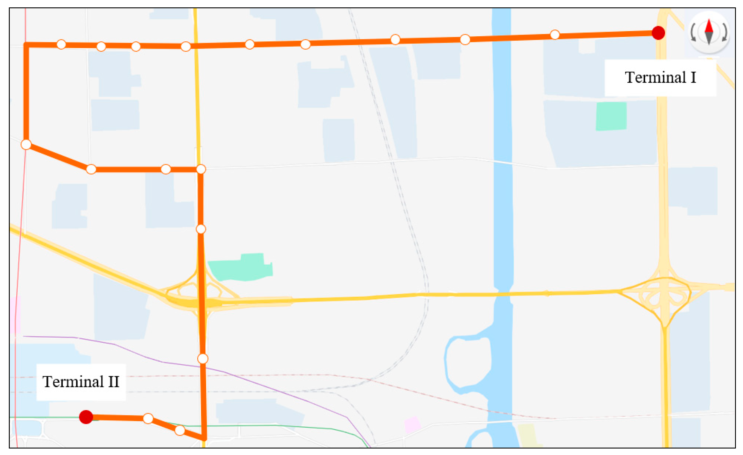
4.1. Data Investigation

In this subsection, an actual electric bus route in a specific city in China was adopted as the research object and the data from 14 March 2023 were utilized to validate the established method. The route consists of 19 stations, as illustrated in Figure 2. Chargers were deployed in Terminal I. As described in Section 2.1, the process of the AMB running from Terminal I to Terminal II and returning to Terminal I is one trip. The operating mileage of one trip is 17.3 km. The departure time of the first and last trips of the route is 5:30 and 20:30, respectively. The operating time is divided into nine operating periods and the specific operational information of each period is listed in Table 1. The city implements a time-of-use tariff policy, and the related information is presented in Table 2. Table 3 gives the average temperatures for each hour during operation.
The maximum number of cross-sectional passengers on each trip is listed in Appendix A. Referring to the actual condition, we assume that the AMBs are equipped with LiFePO4 batteries. The battery system energy density ( η ) is 140.13 Wh/kg. In actual operation, the rated passenger load for an electric bus on the route is 77, the mass of the bare vehicle (without battery) is 9190 kg, and the purchase costs (without battery) are 522,490 CNY. The rated passenger load for an AMB is 10 [5], thus assuming that the bare mass of an AMB (without battery) is 1193.5 kg (10/77 × 9190 kg), and the purchase costs (without battery) are 67,855.8 CNY (10/77 × 522,490 CNY). The average daily acquisition costs of the infrastructure can be obtained by dividing the acquisition costs by the useful life. The charger acquisition costs are 100,000 CNY and the acquisition costs of the battery are 1400 CNY per kWh. The charger can be used for 10 years. The battery’s useful life is 6 years [29]. Table 4 shows the values of other parameters in the developed model.

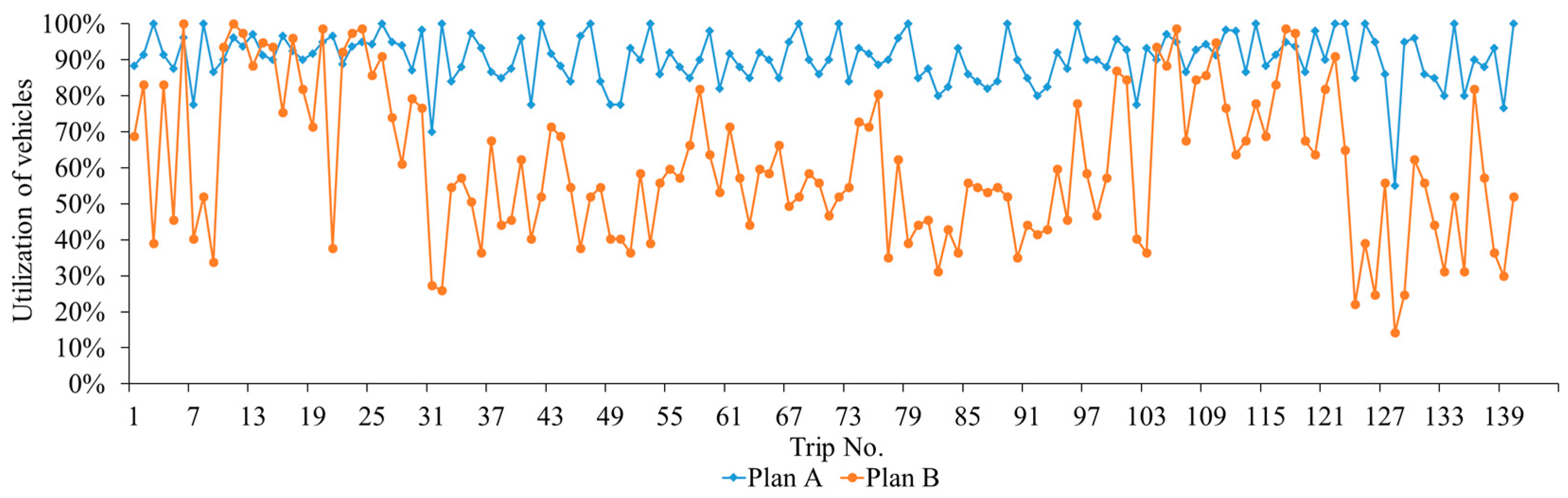
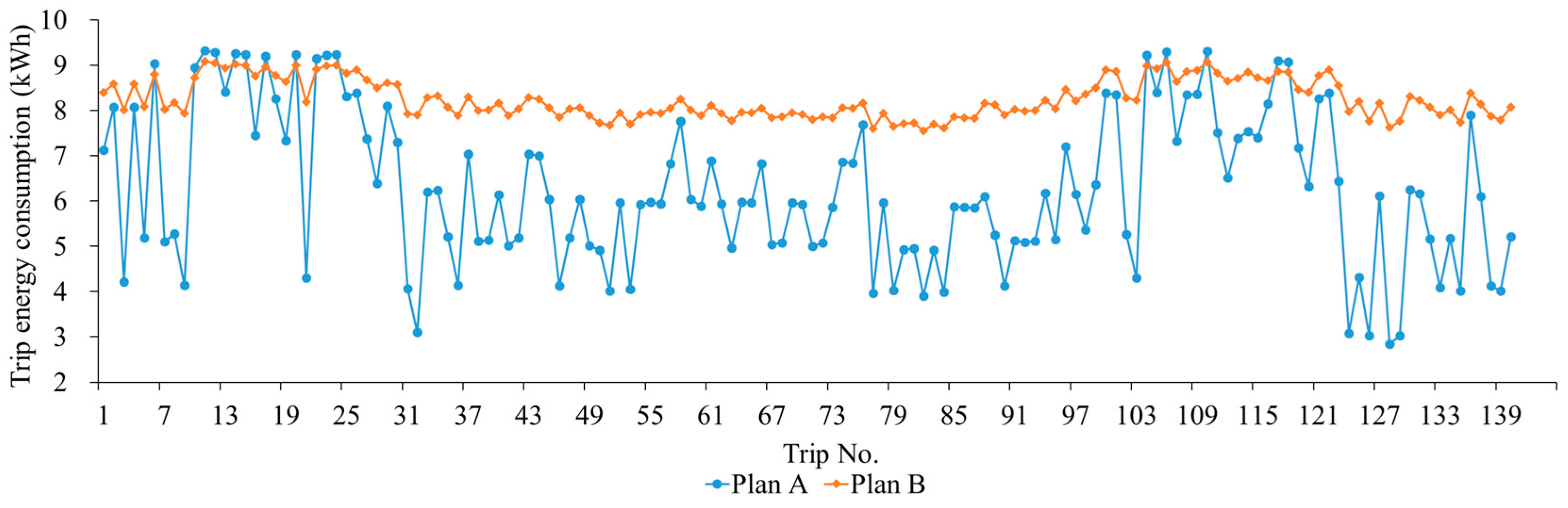
4.2. Optimization Results and Analysis

We used Python 3.8.2 to address the formulated model. For the optimal solution obtained, the route operating costs Z = 4794.302 CNY, the AMB fleet size U = 98, the battery capacity B = 16 kWh, and the number of chargers R = 1. Among them, the charger deployment costs are 27.4 CNY, AMB body acquisition costs are 3036.04 CNY, battery acquisition costs are 1001.952 CNY, and charging costs are 728.91 CNY. It can be seen that the AMB body acquisition costs are the largest expenditure in the route operation, constituting 63.33% of the total operating costs. The charger deployment costs, battery acquisition costs, and charging costs account for 0.57%, 20.90%, and 15.20% of the overall route operating costs, respectively. The charging of AMBs all takes place at night after the end of operation. The AMB dispatching plan is displayed in Table 5.
The suboptimal solution is used to compare with the above optimal solution in this paper. In the suboptimal solution, the route operating costs Z = 4810.822 CNY, the AMB fleet size U = 98, the battery capacity B = 16 kWh, and the number of chargers R = 2. Among them, the charger deployment costs are 54.8 CNY, AMB body acquisition costs are 3036.04 CNY, battery acquisition costs are 1001.952 CNY, and charging costs are 718.03 CNY. Compared with the suboptimal solution, the charging costs of the optimal solution are increased by 10.88 CNY. This is because the charging of AMBs occurs in both the nighttime tariff shoulder period and off-peak period, i.e., 21:00–23:00 and 23:00–6:00. While in the suboptimal solution, the charging of AMBs only occurs in the nighttime tariff off-peak period, i.e., 23:00–6:00. However, the optimal solution reduces the charger deployment costs by 27.4 CNY. Hence, we chose to deploy one charger in the charging station.
We compare the vehicle dispatching plan, charging plan, and charging infrastructure configuration between the proposed method (Plan A) and the current plan using EBs for route operation (Plan B) to verify the effectiveness of the method proposed in this paper.
Plan A: Use AMBs to serve the given trips.
Plan B: Use EBs to serve the given trips. The mass and the purchase costs of the bare EB (without battery) are 9190 kg and 522,490 CNY, respectively. The capacity of an EB is 77 passengers.
As can be seen in Table 6, the route operating costs in Plan A are reduced by 5.92%, equivalent to 301.77 CNY, compared to Plan B. It is apparent that the major reason for the reduction in the route operating costs in Plan A is the significant decrease in the charging costs. This is due to the significant reduction in the route operating energy consumption in Plan A compared to Plan B. The daily route operating energy consumption in Plan B is 1155.79 kWh, whereas the daily route operating energy consumption in Plan A is only 880.16 kWh. Compared to Plan B, the daily route operating energy consumption in Plan A is reduced by 23.85%, approximately equal to 275.63 kWh. Figure 3 illustrates the operational energy consumption for each trip. It is observed that the trip energy consumption of Plan A in the off-peak hours is much lower than that of Plan B. This is because Plan A is able to flexibly adjust the number of vehicles to perform a trip according to passenger demand. During low passenger demand periods, fewer AMBs are needed to complete a trip, vehicle weight is reduced, and thus, trip energy consumption is reduced.
Similarly, as Plan A can flexibly adjust the vehicle capacity of each trip according to passenger demand, the utilization of vehicles in Plan A also increases, especially during off-peak hours. Figure 4 depicts the utilization of vehicles for each trip.
Moreover, we find that the trip energy consumption in Plan A is likely to be higher than that in Plan B, and utilization of vehicles may be lower than that in Plan B during peak hours. This is because the rated passenger load of a vehicle in historical operations is 77, i.e., the maximum historical passenger demand for one trip is 77 passengers, whereas the rated passenger load of an AMB is 10. Plan A will equip eight AMBs for one trip when passenger demand is in the range of [71, 77] during peak hours. In this case, the vehicle weight and vehicle capacity for one trip in Plan A are larger than in Plan B, resulting in higher trip energy consumption and lower utilization of vehicles.

5. Conclusions

The emergence of AMBs is of great significance in enhancing the sustainability of the urban public transportation system. This study develops a collaborative optimization method for bus route operating AMBs to concurrently determine the AMB dispatching plan, charging scheduling plan, and charging infrastructure configuration scheme, under the circumstance that the first vehicle of the coupled AMBs provides energy during the entire trip. A hybrid intelligent algorithm was designed to resolve the established model. Numerical experiments were carried out utilizing the data of an actual EB route. The findings are as follows:
(i)
The collaborative optimization method developed in this paper can flexibly adjust the number of vehicles to perform a trip according to passenger demand, leading to lower vehicle weight during off-peak hours. It realizes decreased trip energy consumption, improved vehicle utilization, and reduced route operating costs.
(ii)
Utilizing AMB for bus routes can effectively reduce daily operating costs and operational energy consumption, compared to using conventional EB. The former can be reduced by 5.92%, approximately 301.77 CNY. The latter can be reduced by 23.85%, approximately equal to 275.63 kWh.
However, there are some limitations to this study. We neglected the impact of ambient temperature on people’s choice of public transport traveling mode [45]. The coupling and decoupling operations of AMBs at any stops were not considered. Future work is required to further discuss the above issues to address the spatial fluctuations in passenger demand, which can further promote the realization of a sustainable urban public transportation system. In addition, for future research, the proposed collaborative optimization method can be potentially extended to multiple routes and multiple charging modes (e.g., multiple vehicles of the coupled AMBs providing energy jointly during the trip). An exact efficient solution algorithm will be studied in the future.

Author Contributions

Conceptualization, A.C. and Y.C.; methodology, Y.C. and C.W.; software, Y.B.; validation, A.C., C.W. and Y.B.; investigation, Y.C.; data curation, Y.C.; writing—original draft preparation, A.C. and C.W.; writing—review and editing, Y.B.; visualization, Y.B. All authors have read and agreed to the published version of the manuscript.

Funding

This research was funded by the Youth Science and Technology Innovation and Entrepreneurship Outstanding Talent (Team) Project of Jilin Province, grant number 20230508048RC.

Institutional Review Board Statement

Not applicable.

Informed Consent Statement

Not applicable.

Data Availability Statement

Data will be made available upon reasonable request.

Conflicts of Interest

The authors declare no conflicts of interest.

Appendix A

Table A1. The maximum number of cross-sectional passengers on each trip.
Trip No.Maximum Number of Cross-Sectional Passengers (Pax)Trip No.Maximum Number of Cross-Sectional Passengers (Pax)Trip No.Maximum Number of Cross-Sectional Passengers (Pax)
15348429535
26449319660
33050319745
46451289836
53552459944
677533010067
731544310165
840554610231
926564410328
1072575110472
1177586310568
1275594910676
1368604110752
1473615510865
1572624410966
1658623411073
1774644611159
1863654511249
1955665111352
2076673811460
2129684011553
2271694511664
2375704311776
2476713611875
2566724011952
2670734212049
2757745612163
2847755512270
2961766212350
3059772712417
3121784812530
3220793012619
3342803412743
3444813512811
3539822412919
3628833313048
3752842813143
3834854313234
3935864213324
4048874113440
4131884213524
4240894013663
4355902713744
4453913413828
4542923213923
4629933314040
47409446

References

  1. Liu, Y.; Francis, A.; Hollauer, C.; Lawson, M.C.; Shaikh, O.; Cotsman, A.; Bhardwaj, K.; Banboukian, A.; Li, M.; Webb, A.; et al. Reliability of electric vehicle charging infrastructure: A cross-lingual deep learning approach. Commun. Transp. Res. 2023, 3, 100095. [Google Scholar] [CrossRef]
  2. Ji, J.; Bie, Y.; Shi, H.; Wang, L. Energy-saving speed profile planning for a connected and automated electric bus considering motor characteristic. J. Clean. Prod. 2024, 448, 141721. [Google Scholar] [CrossRef]
  3. Zhang, Z.; Tafreshian, A.; Masoud, N. Modular transit: Using autonomy and modularity to improve performance in public transportation. Transp. Res. Part E Logist. Transp. Rev. 2020, 141, 102033. [Google Scholar] [CrossRef]
  4. Khan, Z.S.; He, W.; Menéndez, M. Application of modular vehicle technology to mitigate bus bunching. Transp. Res. Part C Emerg. Technol. 2023, 146, 103953. [Google Scholar] [CrossRef]
  5. Liu, X.; Qu, X.; Ma, X. Improving flex-route transit services with modular autonomous vehicles. Transp. Res. Part E Logist. Transp. Rev. 2021, 149, 102331. [Google Scholar] [CrossRef]
  6. Ji, Y.; Liu, B.; Shen, Y.; Du, Y. Scheduling strategy for transit routes with modular autonomous vehicles. Int. J. Transp. Sci. Technol. 2021, 10, 121–135. [Google Scholar] [CrossRef]
  7. Liu, Z.; de Almeida Correia, G.H.; Ma, Z.; Li, S.; Ma, X. Integrated optimization of timetable, bus formation, and vehicle scheduling in autonomous modular public transport systems. Transp. Res. Part C Emerg. Technol. 2023, 155, 104306. [Google Scholar] [CrossRef]
  8. He, Y.; Liu, Z.; Song, Z. Joint optimization of electric bus charging infrastructure, vehicle scheduling, and charging management. Transp. Res. Part D Transp. Environ. 2023, 117, 103653. [Google Scholar] [CrossRef]
  9. He, H.; Sun, F.; Wang, Z.; Lin, C.; Zhang, C.; Xiong, R.; Deng, J.; Zhu, X.; Xie, P.; Zhang, S.; et al. China’s battery electric vehicles lead the world: Achievements in technology system architecture and technological breakthroughs. Green Energy Intell. Transp. 2022, 1, 100020. [Google Scholar] [CrossRef]
  10. Lin, Y.; Zhang, K.; Shen, Z.J.M.; Ye, B.; Miao, L. Multistage large-scale charging station planning for electric buses considering transportation network and power grid. Transp. Res. Part C Emerg. Technol. 2019, 107, 423–443. [Google Scholar] [CrossRef]
  11. Cong, Y.; Wang, H.; Bie, Y.; Wu, J. Double-battery configuration method for electric bus operation in cold regions. Transp. Res. Part E Logist. Transp. Rev. 2023, 180, 103362. [Google Scholar] [CrossRef]
  12. Qu, X.; Wang, S.; Niemeier, D. On the urban-rural bus transit system with passenger-freight mixed flow. Commun. Transp. Res. 2022, 2, 100054. [Google Scholar] [CrossRef]
  13. Zeng, Z.; Qu, X. What’s next for battery-electric bus charging systems. Commun. Transp. Res. 2023, 3, 100094. [Google Scholar] [CrossRef]
  14. Perumal, S.S.; Lusby, R.M.; Larsen, J. Electric bus planning & scheduling: A review of related problems and methodologies. Eur. J. Oper. Res. 2022, 301, 395–413. [Google Scholar]
  15. Chen, G.; Hu, D.; Chien, S.; Guo, L.; Liu, M. Optimizing wireless charging locations for battery electric bus transit with a genetic algorithm. Sustainability 2020, 12, 8971. [Google Scholar] [CrossRef]
  16. He, J.; Yan, N.; Zhang, J.; Yu, Y.; Wang, T. Battery electric buses charging schedule optimization considering time-of-use electricity price. J. Intell. Connect. Veh. 2022, 5, 138–145. [Google Scholar] [CrossRef]
  17. Xylia, M.; Leduc, S.; Patrizio, P.; Silveira, S.; Kraxner, F. Developing a dynamic optimization model for electric bus charging infrastructure. Transp. Res. Procedia 2017, 27, 776–783. [Google Scholar] [CrossRef]
  18. Sang, X.; Yu, X.; Chang, C.T.; Liu, X. Electric bus charging station site selection based on the combined DEMATEL and PROMETHEE-PT framework. Comput. Ind. Eng. 2022, 168, 108116. [Google Scholar] [CrossRef]
  19. Wang, Y.; Huang, Y.; Xu, J.; Barclay, N. Optimal recharging scheduling for urban electric buses: A case study in Davis. Transp. Res. Part E Logist. Transp. Rev. 2017, 100, 115–132. [Google Scholar] [CrossRef]
  20. Hu, H.; Du, B.; Liu, W.; Perez, P. A joint optimisation model for charger locating and electric bus charging scheduling considering opportunity fast charging and uncertainties. Transp. Res. Part C Emerg. Technol. 2022, 141, 103732. [Google Scholar] [CrossRef]
  21. Liu, X.; Qu, X.; Ma, X. Optimizing electric bus charging infrastructure considering power matching and seasonality. Transp. Res. Part D Transp. Environ. 2021, 100, 103057. [Google Scholar] [CrossRef]
  22. McCabe, D.; Ban, X.J. Optimal locations and sizes of layover charging stations for electric buses. Transp. Res. Part C Emerg. Technol. 2023, 152, 104157. [Google Scholar] [CrossRef]
  23. Uslu, T.; Kaya, O. Location and capacity decisions for electric bus charging stations considering waiting times. Transp. Res. Part D Transp. Environ. 2021, 90, 102645. [Google Scholar] [CrossRef]
  24. Momenitabar, M.; Ebrahimi, Z.D.; Bengtson, K. Optimal placement of battery electric bus charging stations considering energy storage technology: Queuing modeling approach. Transp. Res. Rec. 2023, 2677, 663–672. [Google Scholar] [CrossRef]
  25. Das, P.; Kayal, P. An advantageous charging/discharging scheduling of electric vehicles in a PV energy enhanced power distribution grid. Green Energy Intell. Transp. 2024, 3, 100170. [Google Scholar] [CrossRef]
  26. Guschinsky, N.; Kovalyov, M.Y.; Rozin, B.; Brauner, N. Fleet and charging infrastructure decisions for fast-charging city electric bus service. Comput. Oper. Res. 2021, 135, 105449. [Google Scholar] [CrossRef]
  27. Ke, B.R.; Chung, C.Y.; Chen, Y.C. Minimizing the costs of constructing an all plug-in electric bus transportation system: A case study in Penghu. Appl. Energy 2016, 177, 649–660. [Google Scholar] [CrossRef]
  28. Liu, Z.; Song, Z.; He, Y. Planning of fast-charging stations for a battery electric bus system under energy consumption uncertainty. Transp. Res. Rec. 2018, 2672, 96–107. [Google Scholar] [CrossRef]
  29. He, Y.; Song, Z.; Liu, Z. Fast-charging station deployment for battery electric bus systems considering electricity demand charges. Sustain. Cities Soc. 2019, 48, 101530. [Google Scholar] [CrossRef]
  30. Alwesabi, Y.; Wang, Y.; Avalos, R.; Liu, Z. Electric bus scheduling under single depot dynamic wireless charging infrastructure planning. Energy 2020, 213, 118855. [Google Scholar] [CrossRef]
  31. Liu, X.; Liu, X.; Zhang, X.; Zhou, Y.; Chen, J.; Ma, X. Optimal location planning of electric bus charging stations with integrated photovoltaic and energy storage system. Comput. Aided Civ. Infrastruct. Eng. 2022, 38, 1424–1446. [Google Scholar] [CrossRef]
  32. Gong, M.; Hu, Y.; Chen, Z.; Li, X. Transfer-based customized modular bus system design with passenger-route assignment optimization. Transp. Res. Part E Logist. Transp. Rev. 2021, 153, 102422. [Google Scholar] [CrossRef]
  33. Dakic, I.; Yang, K.; Menendez, M.; Chow, J.Y. On the design of an optimal flexible bus dispatching system with modular bus units: Using the three-dimensional macroscopic fundamental diagram. Transp. Res. Part B Methodol. 2021, 148, 38–59. [Google Scholar] [CrossRef]
  34. Wu, J.; Kulcsár, B.; Qu, X. A modular, adaptive, and autonomous transit system (MAATS): An in-motion transfer strategy and performance evaluation in urban grid transit networks. Transp. Res. Part A Policy Pract. 2021, 151, 81–98. [Google Scholar] [CrossRef]
  35. Li, Q.; Li, X. Trajectory optimization for autonomous modular vehicle or platooned autonomous vehicle split operations. Transp. Res. Part E Logist. Transp. Rev. 2023, 176, 103115. [Google Scholar] [CrossRef]
  36. Chen, Z.; Li, X.; Zhou, X. Operational design for shuttle systems with modular vehicles under oversaturated traffic: Discrete modeling method. Transp. Res. Part B Methodol. 2019, 122, 1–19. [Google Scholar] [CrossRef]
  37. Chen, Z.; Li, X.; Zhou, X. Operational design for shuttle systems with modular vehicles under oversaturated traffic: Continuous modeling method. Transp. Res. Part B Methodol. 2020, 132, 76–100. [Google Scholar] [CrossRef]
  38. Shi, X.; Chen, Z.; Pei, M.; Li, X. Variable-capacity operations with modular transits for shared-use corridors. Transp. Res. Rec. 2020, 2674, 230–244. [Google Scholar] [CrossRef]
  39. Pei, M.; Lin, P.; Du, J.; Li, X.; Chen, Z. Vehicle dispatching in modular transit networks: A mixed-integer nonlinear programming model. Transp. Res. Part E Logist. Transp. Rev. 2021, 147, 102240. [Google Scholar] [CrossRef]
  40. Tian, Q.; Lin, Y.H.; Wang, D.Z.; Liu, Y. Planning for modular-vehicle transit service system: Model formulation and solution methods. Transp. Res. Part C Emerg. Technol. 2022, 138, 103627. [Google Scholar] [CrossRef]
  41. Tian, Q.; Lin, Y.H.; Wang, D.Z. Joint scheduling and formation design for modular-vehicle transit service with time-dependent demand. Transp. Res. Part C Emerg. Technol. 2023, 147, 103986. [Google Scholar] [CrossRef]
  42. Guo, R.; Guan, W.; Vallati, M.; Zhang, W. Modular autonomous electric vehicle scheduling for customized on-demand bus services. IEEE Trans. Intell. Transp. Syst. 2023, 24, 10055–10066. [Google Scholar] [CrossRef]
  43. Bie, Y.; Cong, Y.; Yang, M.; Wang, L. Coordinated scheduling of electric buses for multiple routes considering stochastic travel times. J. Transp. Eng. Part A Syst. 2023, 149, 04023069. [Google Scholar] [CrossRef]
  44. Ji, J.; Bie, Y.; Zeng, Z.; Wang, L. Trip energy consumption estimation for electric buses. Commun. Transp. Res. 2022, 2, 100069. [Google Scholar] [CrossRef]
  45. Li, Z.; Su, S.; Jin, X.; Xia, M.; Chen, Q.; Yamashita, K. Stochastic and distributed optimal energy management of active distribution network with integrated office buildings. CSEE J. Power Energy Syst. 2024, 10, 504–517. [Google Scholar]
Figure 1. Schematic diagram of multiple AMBs performing a trip together.
Sustainability 16 03316 g001
Figure 2. Layout of the real route.
Sustainability 16 03316 g002
Figure 3. Trip energy consumption.
Sustainability 16 03316 g003
Figure 4. Utilization of vehicles.
Sustainability 16 03316 g004
Table 1. The specific operational information of each period.
IndexTime PeriodHeadway (min)Number of TripsTravel Time (min)
15:30–6:3061053
26:30–8:3052458
38:30–10:0061555
410:00–15:0083853
515:00–16:0061058
616:00–17:3051863
717:30–18:3061058
818:30–19:308853
919:30–20:3010750
Table 2. Time-of-use tariff schedule.
IndexTime PeriodElectricity Price (CNY/kWh)
16:00–9:001.0866
29:00–11:301.3574
311:30–15:301.0866
415:30–21:001.3574
521:00–23:001.0866
623:00–6:000.8158
Table 3. Average temperatures for each hour during operation.
IndexTime PeriodAverage Temperature (°C)IndexTime PeriodAverage Temperature (°C)
105:00–06:00−3914:00–15:003
206:00–07:00−31015:00–16:002
307:00–08:00−21116:00–17:001
408:00–09:0001217:00–18:000
509:00–10:0011318:00–19:00−2
610:00–11:0021419:00–20:00−3
711:00–12:0021520:00–21:00−4
813:00–14:003
Table 4. Values of some parameters of the developed model.
ParameterValueParameterValue
c pile 27.4 CNY SOC min 20%
c AMB 30.98 CNY SOC max 95%
c battery 0.639 CNY B min 10 kWh
P120 kW B max 60 kWh
M p a s 60 kg
Table 5. AMB dispatching plan.
Trip No.AMB No.Wi (kWh)Trip No.AMB No.Wi (kWh)
11–2–3–4–5–67.137196–67–28–365.01
27–8–24–10–11–12–138.087221–18–19–205.08
315–14–164.227332–33–34–30–315.86
474–18–19–20–21–22–238.087417–60–57–58–59–736.86
59–25–26–275.197565–66–25–63–64–296.84
628–29–30–31–32–33–34–359.037626–43–70–71–83–69–487.68
736–37–38–395.117756–61–553.97
840–41–42–435.287815–52–53–54–145.97
944–45–464.147911–12–94.03
1047–48–1–2–3–4–5–68.958010–84–40–474.93
1149–7–8–9–10–11–12–139.328168–37–38–394.95
1250–51–52–53–54–14–15–169.29823–2–353.91
1355–56–57–58–59–60–618.418345–46–81–824.91
1462–17–18–19–20–21–22–239.258479–80–783.99
1563–64–65–66–24–25–26–279.248576–77–75–16–505.88
1629–30–31–32–33–347.458690–86–87–88–895.86
1735–67–28–36–37–38–39–689.208795–91–92–93–945.85
1841–40–69–42–43–70–718.268842–27–22–23–516.10
1972–73–74–75–76–777.348985–1–41–725.25
2078–79–80–81–82–44–45–469.239022–62–174.13
214–5–64.309120–21–18–195.13
2248–83–84–47–85–1–2–39.159239–68–37–385.09
2313–49–7–8–9–10–11–129.229365–29–44–645.11
2416–50–51–52–53–54–14–159.23945–49–7–6–46.17
2561–55–56–57–58–59–608.319531–66–25–635.15
2622–62–17–18–19–20–218.389658–59–73–74–60–577.20
2725–63–64–65–66–247.389753–54–14–15–526.16
2830–31–32–33–346.399864–29–26–635.37
2967–28–36–37–38–39–688.109969–48–3–2–356.37
3071–83–69–42–43–707.3010082–45–46–81–11–12–98.38
3175–76–774.0710189–90–86–41–72–65–308.34
3274–733.1010210–84–40–475.27
3381–82–44–45–466.2010332–33–344.31
3440–84–47–85–16.2310494–95–91–85–1–56–61–559.22
359–10–11–125.2110519–20–21–18–79–80–788.40
3680–78–794.1410623–25–27–22–51–22–62–179.29
3751–52–53–54–14–157.0410738–39–68–37–56–617.33
3822–23–25–275.1210897–96–67–28–36–55–88.34
3957–58–59–605.1310998–42–43–70–71–83–768.36
4034–30–31–32–336.1411059–45–74–60–57–58–77–509.31
4118–19–20–215.0211154–46–15–52–53–167.52
4237–38–39–685.191124–5–49–7–66.51
4370–71–83–69–42–437.0411387–31–66–26–63–817.39
4466–25–63–64–65–297.0011488–69–48–3–2–357.53
4546–81–82–44–456.0311592–64–29–10–63–827.40
466–4–54.1211693–45–46–81–11–12–338.15
478–13–49–75.1911773–89–90–86–41–72–65–309.09
482–3–35–41–726.0311814–19–20–21–18–79–80–789.08
4996–67–28–365.0211975–11–12–9–32–847.17
5012–9–10–114.9212044–40–47–61–556.33
5117–61–554.0212124–94–95–91–85–1–568.26
5233–34–30–31–325.9612283–34–42–43–70–71–238.38
5337–38–394.0612385–27–22–51–226.44
5452–53–54–14–155.9312454–623.08
5584–40–47–85–15.9812588–68–374.32
5627–22–23–26–515.9412638–563.03
5760–57–58–59–73–746.8212776–97–96–67–286.11
5843–70–71–83–69–42–487.7612898–362.85
5945–46–81–82–446.0312992–613.03
6077–75–76–16–505.8913064–36–55–8–616.25
6164–66–25–63–65–296.8913118–4–5–49–76.16
6256–2–35–41–725.9413269–6–46–155.17
6221–18–19–204.9713377–57–584.10
6486–87–88–89–905.9813495–52–53–165.17
6591–92–93–94–955.9613525–46–814.01
6679–80–78–22–62–176.821363–29–10–63–82–45–117.90
6768–37–38–395.0513790–86–41–72–656.10
6811–12–9–105.0813839–21–794.12
696–4–5–49–75.9613965–44–404.02
7056–61–55–8–135.9314020–88–68–375.21
Table 6. Comparison of results under two plans.
PlanPlan APlan B
U9813
B (kWh)16120
R12
Z (CNY)4794.3025096.07
Z1 (CNY)27.454.8
Z2 (CNY)3036.043101.54
Z3 (CNY)1001.952996.84
Z4 (CNY)728.91942.89
Disclaimer/Publisher’s Note: The statements, opinions and data contained in all publications are solely those of the individual author(s) and contributor(s) and not of MDPI and/or the editor(s). MDPI and/or the editor(s) disclaim responsibility for any injury to people or property resulting from any ideas, methods, instructions or products referred to in the content.

